Author Archives: Research Blog

Announcing TensorFlow 0.8 – now with distributed computing support!


Google uses machine learning across a wide range of its products. In order to continually improve our models, it's crucial that the training process be as fast as possible. One way to do this is to run TensorFlow across hundreds of machines, which shortens the training process for some models from weeks to hours, and allows us to experiment with models of increasing size and sophistication. Ever since we released TensorFlow as an open-source project, distributed training support has been one of the most requested features. Now the wait is over.

Today, we're excited to release TensorFlow 0.8 with distributed computing support, including everything you need to train distributed models on your own infrastructure. Distributed TensorFlow is powered by the high-performance gRPC library, which supports training on hundreds of machines in parallel. It complements our recent announcement of Google Cloud Machine Learning, which enables you to train and serve your TensorFlow models using the power of the Google Cloud Platform.

To coincide with the TensorFlow 0.8 release, we have published a distributed trainer for the Inception image classification neural network in the TensorFlow models repository. Using the distributed trainer, we trained the Inception network to 78% accuracy in less than 65 hours using 100 GPUs. Even small clusters—or a couple of machines under your desk—can benefit from distributed TensorFlow, since adding more GPUs improves the overall throughput, and produces accurate results sooner.
TensorFlow can speed up Inception training by a factor of 56, using 100 GPUs.
The distributed trainer also enables you to scale out training using a cluster management system like Kubernetes. Furthermore, once you have trained your model, you can deploy to production and speed up inference using TensorFlow Serving on Kubernetes.

Beyond distributed Inception, the 0.8 release includes new libraries for defining your own distributed models. TensorFlow's distributed architecture permits a great deal of flexibility in defining your model, because every process in the cluster can perform general-purpose computation. Our previous system DistBelief (like many systems that have followed it) used special "parameter servers" to manage the shared model parameters, where the parameter servers had a simple read/write interface for fetching and updating shared parameters. In TensorFlow, all computation—including parameter management—is represented in the dataflow graph, and the system maps the graph onto heterogeneous devices (like multi-core CPUs, general-purpose GPUs, and mobile processors) in the available processes. To make TensorFlow easier to use, we have included Python libraries that make it easy to write a model that runs on a single process and scales to use multiple replicas for training.

This architecture makes it easier to scale a single-process job up to use a cluster, and also to experiment with novel architectures for distributed training. As an example, my colleagues have recently shown that synchronous SGD with backup workers, implemented in the TensorFlow graph, achieves improved time-to-accuracy for image model training.

The current version of distributed computing support in TensorFlow is just the start. We are continuing to research ways of improving the performance of distributed training—both through engineering and algorithmic improvements—and will share these improvements with the community on GitHub. However, getting to this point would not have been possible without help from the following people:
  • TensorFlow training libraries - Jianmin Chen, Matthieu Devin, Sherry Moore and Sergio Guadarrama
  • TensorFlow core - Zhifeng Chen, Manjunath Kudlur and Vijay Vasudevan
  • Testing - Shanqing Cai
  • Inception model architecture - Christian Szegedy, Sergey Ioffe, Vincent Vanhoucke, Jonathon Shlens and Zbigniew Wojna
  • Project management - Amy McDonald Sandjideh
  • Engineering leadership - Jeff Dean and Rajat Monga

All of Google’s CS Education Programs and Tools in One Place


(Cross-posted on the Google for Education Blog)

Interest in computer science education is growing rapidly; even the President of the United States has spoken of the importance of giving every student an opportunity to learn computer science. Google has been a supportive partner in these efforts by developing high-quality learning programs, educational tools and resources to advance new approaches in computer science education. To make it easier for all students and educators to access this information, today we’re launching a CS EDU website that specifically outlines our initiatives in CS education.
The President’s call to action is grounded in economic realities coupled with a lack of access and ongoing system inequities. There is an increasing need for computer science skills in the workforce, with the Bureau of Labor Statistics estimating that there will be more than 1.3 million job openings in computer and mathematical occupations by 2022. The majority of these jobs will require at least a Bachelor’s degree in Computer Science or in Information Technology, yet the U.S. is only producing 16,000 CS undergraduates per year.

One of the reasons there are so few computer science graduates is that too few students have the opportunity to study computer science in high school. Google’s research shows that only 25% of U.S. schools currently offer CS with programming or coding, despite the fact that 91% of parents want their children to learn computer science. In addition, schools with higher percentages of students living in households below the poverty line are even less likely to offer rigorous computer science courses.

Increasing access to computer science for all learners requires tremendous commitment from a wide range of stakeholders, and we strive to be a strong supportive partner of these efforts. Our new CS EDU website shows all the ways Google is working to address the need for improved access to high quality computer science learning in formal and informal education. Some current programs you’ll find there include:

  • CS First: providing more than 360,000 middle school students with an opportunity to create technology through free computer science clubs
  • Exploring Computational Thinking: sharing more than 130 lesson plans aligned to international standards for students aged 8 to 18
  • igniteCS: offering support and mentoring to address the retention problem in diverse student populations at the undergraduate level in more than 40 universities and counting
  • Blockly and other programming tools powering Code.org’s Hour of Code (2 million users)
  • Google’s Made with Code: movement that inspires millions of girls to learn to code and to see it as a means to pursue their dream careers (more than 10 million unique visitors)
  • ...and many more!

Computer science education is a pathway to innovation, to creativity and to exciting career opportunities, and Google believes that all students deserve these opportunities. That is why we are committed to developing programs, resources, tools and community partnerships that make computer science engaging and accessible for all students. With the launch of our CS EDU website, all of these programs are at your fingertips.

Genomic Data Processing on Google Cloud Platform


Today we hear from Broad Institute of MIT and Harvard about how their researchers and software engineers are collaborating closely with the Google Genomics team on large-scale genomic data analysis. They’ve already reduced the time and cost for whole genome processing by several fold, helping researchers think even bigger. Broad’s open source tools, developed in close collaboration with Google Genomics, will also be made available to the wider research community.
– Jonathan Bingham, Product Manager, Google Genomics


Dr. Stacey Gabriel, Director of the
Genomics Platform at the Broad Institute
As one of the largest genome sequencing centers in the world, the Broad Institute of MIT and Harvard generates a lot of data. Our DNA sequencers produce more than 20 Terabytes (TB) of genomic data per day, and they run 365 days a year. Moreover, our rate of data generation is not only growing, but accelerating – our output increased more than two-fold last year, and nearly two-fold the previous year. We are not alone in facing this embarrassment of riches; across the whole genomics community, the rate of data production is doubling about every eight months with no end in sight.

Here at Broad, our team of software engineers and methods developers have spent the last year working to re-architect our production sequencing environment for the cloud. This has been no small feat, especially as we had to build the plane while we flew it! It required an entirely new system for developing and deploying pipelines (which we call Cromwell), as well as a new framework for wet lab quality control that uncouples data generation from data processing.
Courtesy: Broad Institute of MIT and Harvard
Last summer Broad and Google announced a collaboration to develop a safe, secure and scalable cloud computing infrastructure capable of storing and processing enormous datasets. We also set out to build cloud-supported tools to analyze such data and unravel long-standing mysteries about human health. Our engineers collaborate closely; we teach them about genomic data science and genomic data engineering, and they teach us about cloud computing and distributed systems. To us, this is a wonderful model for how a basic research institute can productively collaborate with industry to advance science and medicine. Both groups move faster and go further by working together.

As of today, the largest and most important of our production pipelines, the Whole Genome Sequencing Pipeline, has been completely ported to the Google Cloud Platform (GCP). We are now beginning to run production jobs on GCP and will be switching over entirely this month. This switch has proved to be a very cost-effective decision. While the conventional wisdom is that public clouds can be more expensive, our experience is that cloud is dramatically cheaper. Consider the curve below that my colleague Kristian Cibulskis recently showed at GCP NEXT:
Out of the box, the cost of running the Genome Analysis Toolkit (GATK) best practices pipeline on a 30X-coverage whole genome was roughly the same as the cost of our on-premise infrastructure. Over a period of a few months, however, we developed techniques that allowed us to really reduce costs: We learned how to parallelize the computationally intensive steps like aligning DNA sequences against a reference genome. We also optimized for GCP’s infrastructure to lower costs by using features such as Preemptible VMs. After doing these optimizations, our production whole genome pipeline was about 20% the cost of where we were when we started, saving our researchers millions of dollars, all while reducing processing turnaround time eight-fold.

There is a similar story to be told on storage of the input and output data. Google Cloud Storage Nearline is a medium for storing DNA sequence alignments and raw data. Like most people in genomics, we access genetic variants data every day, but raw DNA sequences only a few times per year, such as when there is a new algorithm that requires raw data or a new assembly of the human genome. Nearline’s price/performance tradeoff is well-suited to data that’s infrequently accessed. By using Nearline, along with some compression tricks, we were able to reduce our storage costs by greater than 50%.

Altogether, we estimate that, by using GCP services for both compute and storage, we will be able to lower the total cost of ownership for storing and processing genomic data significantly relative to our on premise costs. Looking forward, we also see advantages for data sharing, particularly for large multi-group genome projects. An environment where the data can be securely stored and analyzed will solve problems of multiple groups copying and paying for transmission and storage of the same data.

Porting the GATK whole genome pipeline to the cloud is just the starting point. During the coming year, we plan to migrate the bulk of our production pipelines to the cloud, including tools for arrays, exomes, cancer genomes, and RNA-seq. Moreover, our non-exclusive relationship with Google is founded on the principle that our groups can leverage complementary skills to make products that can not only serve the needs of Broad, but also help serve the needs of researchers around the world. Therefore, as we migrate each of our pipelines to the cloud to meet our own needs, we also plan to make them available to the greater genomics community through a Software-as-a-Service model.

This is an exciting time for us at Broad. For more than a decade we have served the genomics community by acting as a hub for data generation; now, we are extending this mission to encompass not only sequencing services, but also data services. We believe that by expanding access to our tools and optimizing our pipelines for the cloud, will enable the community to benefit from the enormous effort we have invested. We look forward to expanding the scope of this mission in the years to come.

Lessons learned while protecting Gmail


Earlier this year in San Francisco, USENIX hosted their inaugural Enigma Conference, which focused on security, privacy and electronic crime through the lens of emerging threats and novel attacks. We were excited to help make this conference happen and to participate in it.

At the conference, we heard from a variety of terrific speakers including:
In addition, we were able to share the lessons we’ve learned about protecting Gmail users since it was launched over a decade ago. Those lessons are summarized in the infographic below (the talk slides are also available).


We were proud to sponsor this year's inaugural Enigma conference, and it is our hope that the core lessons that we have learned over the years can benefit other online products and services. We're looking forward to participating again next year when Enigma returns in 2017. We hope to see you there!

Machine Learning in the Cloud, with TensorFlow


At Google, researchers collaborate closely with product teams, applying the latest advances in Machine Learning to existing products and services - such as speech recognition in the Google app, search in Google Photos and the Smart Reply feature in Inbox by Gmail - in order to make them more useful. A growing number of Google products are using TensorFlow, our open source Machine Learning system, to tackle ML challenges and we would like to enable others do the same.

Today, at GCP NEXT 2016, we announced the alpha release of Cloud Machine Learning, a framework for building and training custom models to be used in intelligent applications.
Machine Learning projects can come in many sizes, and as we’ve seen with our open source offering TensorFlow, projects often need to scale up. Some small tasks are best handled with a local solution running on one’s desktop, while large scale applications require both the scale and dependability of a hosted solution. Google Cloud Machine Learning aims to support the full range and provide a seamless transition from local to cloud environment.

The Cloud Machine Learning offering allows users to run custom distributed learning algorithms based on TensorFlow. In addition to the deep learning capabilities that power Cloud Translate API, Cloud Vision API, and Cloud Speech API, we provide easy-to-adopt samples for common tasks like linear regression/classification with very fast convergence properties (based on the SDCA algorithm) and building a custom image classification model with few hundred training examples (based on the DeCAF algorithm).

We are excited to bring the best of Google Research to Google Cloud Platform. Learn more about this release and more from GCP Next 2016 on the Google Cloud Platform blog.

Announcing the 2016 Google PhD Fellows for North America, Europe and the Middle East


Google created the PhD Fellowship program in 2009 to recognize and support outstanding graduate students doing exceptional research in Computer Science and related disciplines. Now in its eighth year, our fellowship program has supported hundreds of future faculty, industry researchers, innovators and entrepreneurs.

Reflecting our continuing commitment to supporting and building relationships with the academic community, we are excited to announce the 39 recipients from North America, Europe and the Middle East. We offer our sincere congratulations to Google’s 2016 Class of PhD Fellows.

Computational Neuroscience
Cameron (Po-Hsuan) Chen, Princeton University
Grace Lindsay, Columbia University
Martino Sorbaro Sindaci, The University of Edinburgh

Human-Computer Interaction
Koki Nagano, University of Southern California
Arvind Satyanarayan, Stanford University
Amy Xian Zhang, Massachusetts Institute of Technology

Machine Learning
Olivier Bachem, Swiss Federal Institute of Technology Zurich
Tianqi Chen, University of Washington
Emily Denton, New York University
Yves-Laurent Kom Samo, University of Oxford
Daniel Jaymin Mankowitz, Technion - Israel Institute of Technology
Lucas Maystre, École Polytechnique Fédérale de Lausanne
Arvind Neelakantan, University of Massachusetts, Amherst
Ludwig Schmidt, Massachusetts Institute of Technology
Shandian Zhe, Purdue University, West Lafayette

Machine Perception, Speech Technology and Computer Vision
Eugen Beck, RWTH Aachen University
Yu-Wei Chao, University of Michigan, Ann Arbor
Wei Liu, University of North Carolina at Chapel Hill
Aron Monszpart, University College London
Thomas Schoeps, Swiss Federal Institute of Technology Zurich
Chia-Yin Tsai, Carnegie Mellon University

Market Algorithms
Hossein Esfandiari, University of Maryland, College Park
Sandy Heydrich, Saarland University - Saarbrucken GSCS
Rad Niazadeh, Cornell University
Sadra Yazdanbod, Georgia Institute of Technology

Mobile Computing
Lei Kang, University of Wisconsin
Tauhidur Rahman, Cornell University
Yuhao Zhu, University of Texas, Austin

Natural Language Processing
Tamer Alkhouli, RWTH Aachen University
Jose Camacho Collados, Sapienza - Università di Roma

Privacy and Security
Kartik Nayak, University of Maryland, College Park
Nicolas Papernot, Pennsylvania State University
Damian Vizar, École Polytechnique Fédérale de Lausanne
Xi Wu, University of Wisconsin

Programming Languages and Software Engineering
Marcelo Sousa, University of Oxford

Structured Data and Database Management
Xiang Ren, University of Illinois, Urbana-Champaign

Systems and Networking
Andrew Crotty, Brown University
Ilias Marinos, University of Cambridge
Kay Ousterhout, University of California, Berkeley

Train your own image classifier with Inception in TensorFlow


At the end of last year we released code that allows a user to classify images with TensorFlow models. This code demonstrated how to build an image classification system by employing a deep learning model that we had previously trained. This model was known to classify an image across 1000 categories supplied by the ImageNet academic competition with an error rate that approached human performance. After all, what self-respecting computer vision system would fail to recognize a cute puppy?
Image via Wikipedia
Well, thankfully the image classification model would recognize this image as a retriever with 79.3% confidence. But, more spectacularly, it would also be able to distinguish between a spotted salamander and fire salamander with high confidence – a task that might be quite difficult for those not experts in herpetology. Can you tell the difference?
Images via Wikipedia
The deep learning model we released, Inception-v3, is described in our Arxiv preprint "Rethinking the Inception Architecture for Computer Vision” and can be visualized with this schematic diagram:
Schematic diagram of Inception-v3
As described in the preprint, this model achieves 5.64% top-5 error while an ensemble of four of these models achieves 3.58% top-5 error on the validation set of the ImageNet whole image ILSVRC 2012 classification task. Furthermore, in the 2015 ImageNet Challenge, an ensemble of 4 of these models came in 2nd in the image classification task.

After the release of this model, many people in the TensorFlow community voiced their preference on having an Inception-v3 model that they can train themselves, rather than using our pre-trained model. We could not agree more, since a system for training an Inception-v3 model provides many opportunities, including:
  • Exploration of different variants of this model architecture in order to improve the image classification system.
  • Comparison of optimization algorithms and hardware setups for training this model faster or to a higher degree of predictive performance.
  • Retraining/fine-tuning the Inception-v3 model on a distinct image classification task or as a component of a larger network tasked with object detection or multi-modal learning.
The last topic is often referred to as transfer learning, and has been an area of particular excitement in the field of deep networks in the context of vision. A common prescription to a computer vision problem is to first train an image classification model with the ImageNet Challenge data set, and then transfer this model’s knowledge to a distinct task. This has been done for object detection, zero-shot learning, image captioning, video analysis and multitudes of other applications.

Today we are happy to announce that we are releasing libraries and code for training Inception-v3 on one or multiple GPU’s. Some features of this code include:
  • Training an Inception-v3 model with synchronous updates across multiple GPUs.
  • Employing batch normalization to speed up training of the model.
  • Leveraging many distortions of the image to augment model training.
  • Releasing a new (still experimental) high-level language for specifying complex model architectures, which we call TensorFlow-Slim.
  • Demonstrating how to perform transfer learning by taking a pre-trained Inception-v3 model and fine-tuning it for another task.
We can train a model from scratch to its best performance on a desktop with 8 NVIDIA Tesla K40s in about 2 weeks. In order to make research progress faster, we are additionally supplying a new version of a pre-trained Inception-v3 model that is ready to be fine-tuned or adapted to a new task. We demonstrate how to use this model for transfer learning on a simple flower classification task. Hopefully, this provides a useful didactic example for employing this Inception model on wide range of vision tasks.

Want to get started? See the accompanying instructions on how to train, evaluate or fine-tune a network.

Releasing this code has been a huge team effort. These efforts have taken several months with contributions from many individuals spanning research at Google. We wish to especially acknowledge the following people who contributed to this project:
  • Model Architecture – Christian Szegedy, Sergey Ioffe, Vincent Vanhoucke, Jon Shlens and Zbigniew Wojna
  • Systems Infrastructure – Sherry Moore, Martin Wicke, David Andersen, Matthieu Devin, Manjunath Kudlur and Nishant Patil
  • TensorFlow-Slim – Sergio Guadarrama and Nathan Silberman
  • Model Visualization – Fernanda Viégas, Martin Wattenberg and James Wexler

Deep Learning for Robots: Learning from Large-Scale Interaction


While we’ve recently seen great strides in robotic capability, the gap between human and robot motor skills remains vast. Machines still have a very long way to go to match human proficiency even at basic sensorimotor skills like grasping. However, by linking learning with continuous feedback and control, we might begin to bridge that gap, and in so doing make it possible for robots to intelligently and reliably handle the complexities of the real world.

Consider for example this robot from KAIST, which won last year’s DARPA robotics challenge. The remarkably precise and deliberate motions are deeply impressive. But they are also quite… robotic. Why is that? What makes robot behavior so distinctly robotic compared to human behavior? At a high level, current robots typically follow a sense-plan-act paradigm, where the robot observes the world around it, formulates an internal model, constructs a plan of action, and then executes this plan. This approach is modular and often effective, but tends to break down in the kinds of cluttered natural environments that are typical of the real world. Here, perception is imprecise, all models are wrong in some way, and no plan survives first contact with reality.

In contrast, humans and animals move quickly, reflexively, and often with remarkably little advance planning, by relying on highly developed and intelligent feedback mechanisms that use sensory cues to correct mistakes and compensate for perturbations. For example, when serving a tennis ball, the player continually observes the ball and the racket, adjusting the motion of his hand so that they meet in the air. This kind of feedback is fast, efficient, and, crucially, can correct for mistakes or unexpected perturbations. Can we train robots to reliably handle complex real-world situations by using similar feedback mechanisms to handle perturbations and correct mistakes?

While servoing and feedback control have been studied extensively in robotics, the question of how to define the right sensory cue remains exceptionally challenging, especially for rich modalities such as vision. So instead of choosing the cues by hand, we can program a robot to acquire them on its own from scratch, by learning from extensive experience in the real world. In our first experiments with real physical robots, we decided to tackle robotic grasping in clutter.

A human child is able to reliably grasp objects after one year, and takes around four years to acquire more sophisticated precision grasps. However, networked robots can instantaneously share their experience with one another, so if we dedicate 14 separate robots to the job of learning grasping in parallel, we can acquire the necessary experience much faster. Below is a video of our robots practicing grasping a range of common office and household objects:
While initially the grasps are executed at random and succeed only rarely, each day the latest experiences are used to train a deep convolutional neural network (CNN) to learn to predict the outcome of a grasp, given a camera image and a potential motor command. This CNN is then deployed on the robots the following day, in the inner loop of a servoing mechanism that continually adjusts the robot’s motion to maximize the predicted chance of a successful grasp. In essence, the robot is constantly predicting, by observing the motion of its own hand, which kind of subsequent motion will maximize its chances of success. The result is continuous feedback: what we might call hand-eye coordination. Observing the behavior of the robot after over 800,000 grasp attempts, which is equivalent to about 3000 robot-hours of practice, we can see the beginnings of intelligent reactive behaviors. The robot observes its own gripper and corrects its motions in real time. It also exhibits interesting pre-grasp behaviors, like isolating a single object from a group. All of these behaviors emerged naturally from learning, rather than being programmed into the system.
To evaluate whether the system achieves measurable benefit from continuous feedback, we can compare its performance to an open-loop baseline that closer resembles the perception-planning-action loop described previously, albeit with a learned CNN used to determine both the open-loop grasps and the closed-loop servoing trained on the same data. With open-loop grasp selection, the robot chooses a single grasp pose from a single image, and then blindly executes this grasp. This method has a 34% average failure rate on the first 30 picking attempts for this set of office objects:
Incorporating continuous feedback into the system reduces the failures by nearly half, down to 18% from 34%, and produces interesting corrections and adjustments:
Neural networks have made great strides in allowing us to build computer programs that can process images, speech, text, and even draw pictures. However, introducing actions and control adds considerable new challenges, since every decision the network makes will affect what it sees next. Overcoming these challenges will bring us closer to building systems that understand the effects of their actions in the world. If we can bring the power of large-scale machine learning to robotic control, perhaps we will come one step closer to solving fundamental problems in robotics and automation.

The research on robotic hand-eye coordination and grasping was conducted by Sergey Levine, Peter Pastor, Alex Krizhevsky, and Deirdre Quillen, with special thanks to colleagues at Google Research and X who've contributed their expertise and time to this research. An early preprint is available on arXiv.

An Update on fast Transit Routing with Transfer Patterns


What is the best way to get from A to B by public transit? Google Maps is answering such queries for over 20,000 cities and towns in over 70 countries around the world, including large metro areas like New York, São Paulo or Moscow, and some complete countries, such as Japan or Great Britain.
Since its beginnings in 2005 with the single city of Portland, Oregon, the number of cities and countries served by Google’s public transit directions has been growing rapidly. With more and larger regions, the amount of data we need to search in order to provide optimal directions has grown as well. In 2010, the search speed of transit directions made a leap ahead of that growth and became fast enough to update the result while you drag the endpoints. The technique behind that speed-up is the Transfer Patterns algorithm [1], which was created at Google’s engineering office in Zurich, Switzerland, by visiting researcher Hannah Bast and a number of Google engineers.

I am happy to report that this research collaboration has continued and expanded with the Google Focused Research Award on Next-Generation Route Planning. Over the past three years, this grant has supported Hannah Bast’s research group at the University of Freiburg, as well as the research groups of Peter Sanders and Dorothea Wagner at the Karlsruhe Institute of Technology (KIT).

From the project’s numerous outcomes, I’d like to highlight two recent ones that re-examine the Transfer Patterns approach and massively improve it for continent-sized networks: Scalable Transfer Patterns [2] and Frequency-Based Search for Public Transit [3] by Hannah Bast, Sabine Storandt and Matthias Hertel. This blogpost presents the results from these publications.

The notion of a transfer pattern is easy to understand. Suppose you are at a transit stop downtown, call it A, and want to go to some stop B as quickly as possible. Suppose further you brought a printed schedule book but no smartphone. (This sounded plausible only a few years ago!) As a local, you might know that there are only two reasonable options:
  1. Take a tram from A to C, then transfer at C to a bus to B.
  2. Take the direct bus from A to B, which only runs infrequently.
We say the first option has transfer pattern A-C-B, and the second option has transfer pattern A-B. Notice that no in-between stops are mentioned. This is very compact information, much less than the actual schedules, but it makes looking up the schedules significantly faster: Knowing that all optimal trips follow one of these patterns, you only need to look at those lines in the schedule book that provide direct connections from A to C, C to B and A to B. All other lines can safely be ignored: you know you will not miss a better option.

While the basic idea of transfer patterns is indeed that simple, it takes more to make it work in practice. The transfer patterns of all optimal trips have to be computed ahead of time and stored, so that they are available to answer queries. Conceptually, we need transfer patterns for every pair of stops, because any pair could come up in a query. It is perfectly reasonable to compute them for all pairs within one city, or even one metro area that is densely criss-crossed by a transit network comprising, say, a thousand stops, yielding a million of pairs to consider.

As the scale of the problem increases from one metro area to an entire country or continent, this “all pairs” approach rapidly becomes expensive: ten thousand stops (10x more than above) already yield a hundred million pairs (100x more than above), and so on. Also, the individual transfer patterns become quite repetitive: For example, from any stop in Paris, France to any stop in Cologne, Germany, all optimal connections end up using the same few long-distance train lines in the middle, only the local connections to the railway stations depend on the specific pair of stops considered.

However, designated long-distance connections are not the only way to travel between different local networks – they also overlap and connect to each other. For mid-range trips, there is no universally correct rule when to choose a long-distance train or intercity bus, short of actually comparing options with local or regional transit, too.

The Scalable Transfer Patterns algorithm [2] does just that, but in a smart way. For starters, it uses what is known as graph clustering to cut the network into pieces, called 
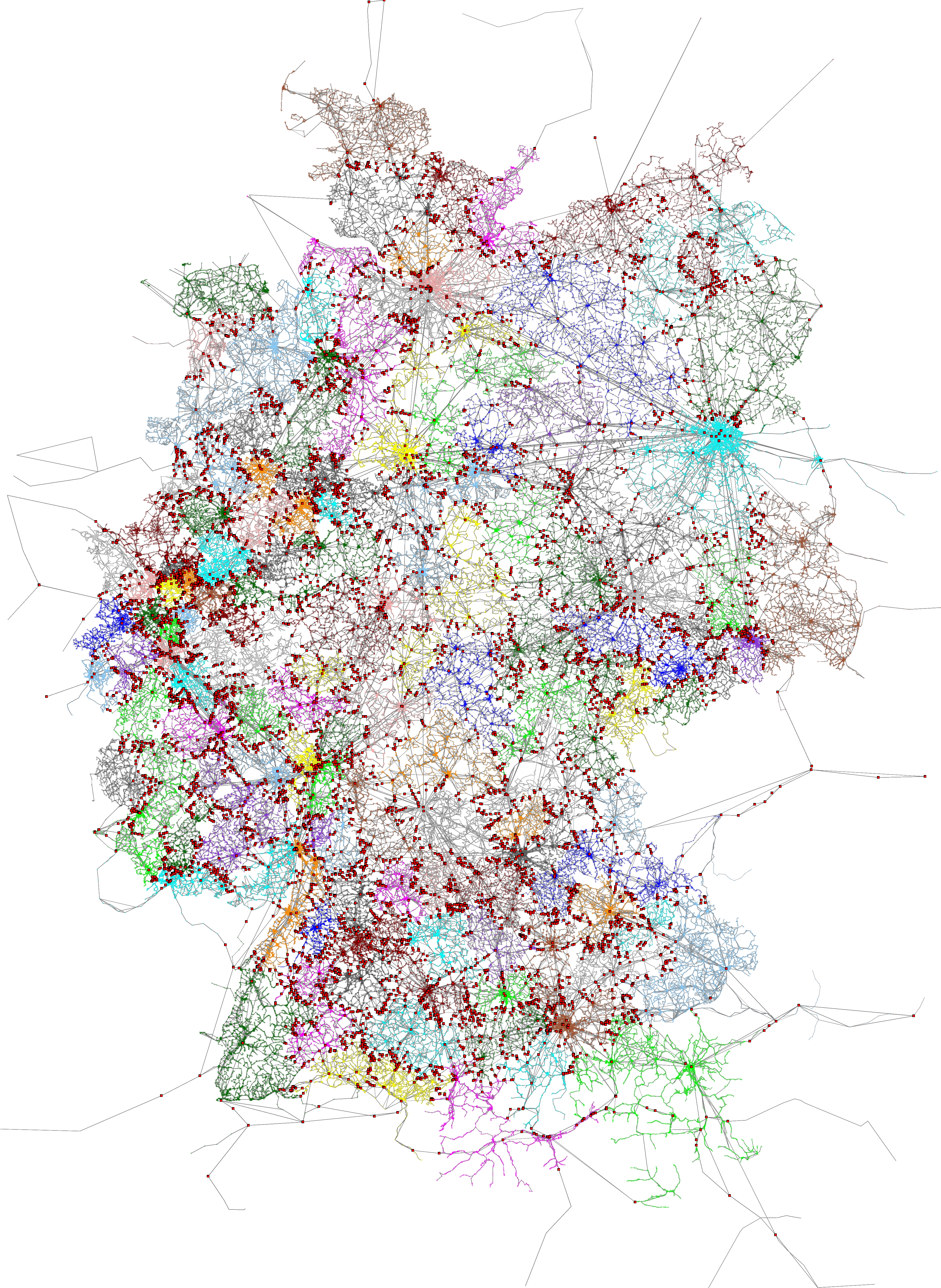
clusters, that have a lot of connections inside but relatively few to the outside. As an example, the figure below (kindly provided by the authors) shows a partitioning of Germany into clusters. The stops highlighted in red are border stops: They connect directly to stops outside the cluster. Notice how they are a small fraction of the total network.
The public transit network of Germany (dots and lines), split into clusters (shown in various colors). Of all 251,763 stops, only 10,886 (4.32%) are boundary stops, highlighted as red boxes. Click here to view the full resolution image.[source: S. Storandt, 2016]
Based on the clustering, the transfer patterns of all optimal connections are computed in two steps.

In step 1, transfer patterns are computed for optimal connections inside each cluster. They are stored for query processing later on, but they also accelerate the search through a cluster in the following step: between the stops on its border, we only need to consider the connections captured in the transfer patterns.

The next figure sketches how the transit network in the cluster around Berlin gets reduced to much fewer connections between border stations. (The central station stands out as a hub, as expected. It is a border station itself, because it has direct connections out of the cluster.)
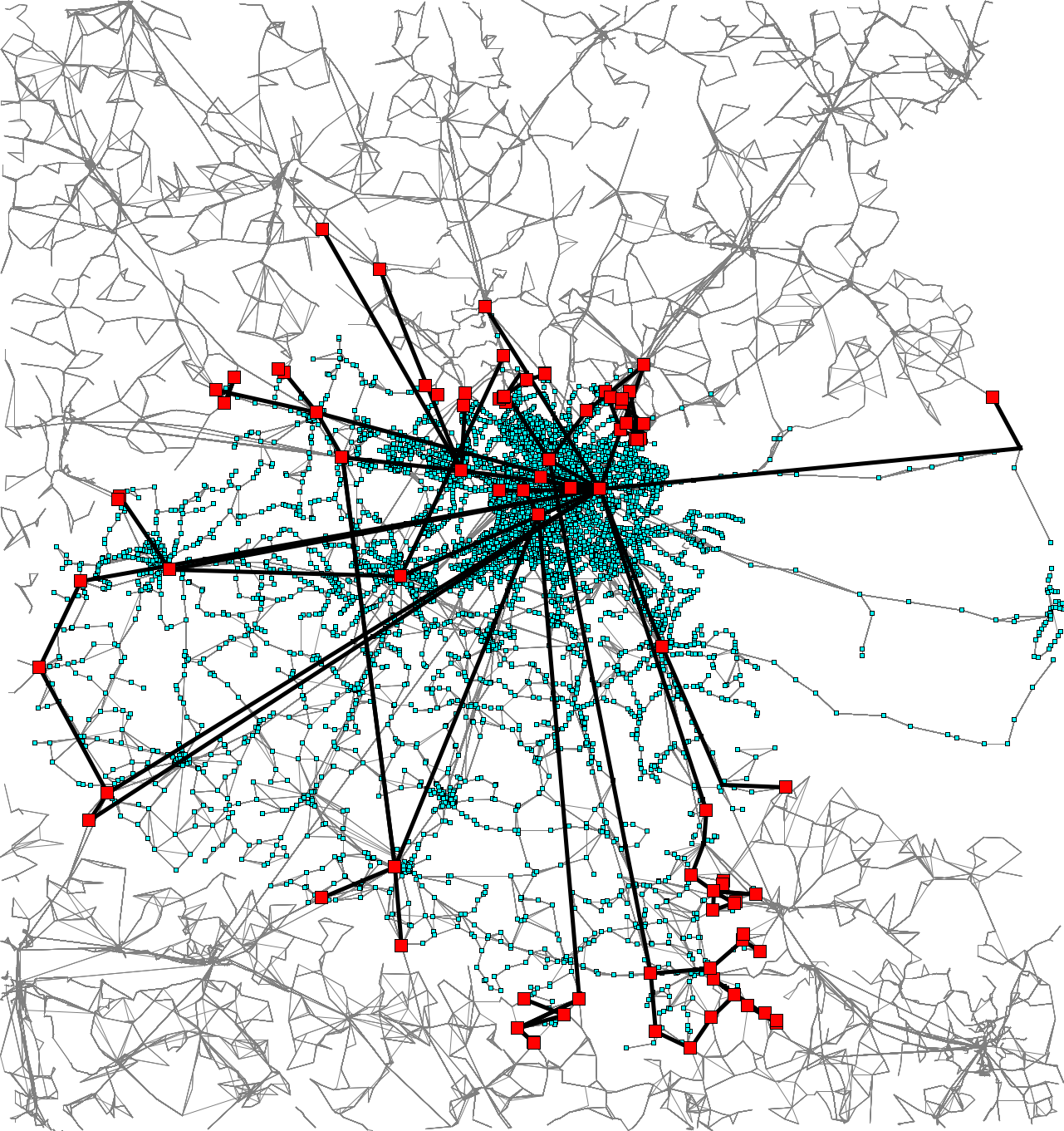
The cluster of public transit connections around Berlin (shown as dots and lines in light blue), its border stops (highlighted as red boxes), and the transfer patterns of optimal connections between border stops (thick black lines; only the most important 111 of 592 are shown to keep the image legible). This cuts out 96.15% of the network (especially a lot of the high-frequency inner city trips, which makes the time savings even bigger). Click here to view the full resolution image. [source: S. Storandt, 2016]
In step 2, transfer patterns can be computed for the entire network, that is, between any pair of clusters. This is done with the following twists:

  • It suffices to consider trips from and to boundary stops of any cluster; the local transfer patterns from step 1 will supply the missing pieces later on.
  • The per-cluster transfer patterns from step 1 greatly accelerate the search across other clusters.
  • The search stops exploring any possible connection between two boundary stops as soon as it gets worse than a connection that sticks to long-distance transit between clusters (which may not always be optimal, but is always quick to compute).

The results of steps 1 and 2 are stored and used to answer queries. For any given query from some A to some B, one can now easily stitch together a network of transfer patterns that covers all optimal connections from A to B. Looking up the direct connections on that small network (like in the introductory example) and finding the best one for the queried time is very fast, even if A and B are far away.

The total storage space needed for this is much smaller than the space that would be needed for all pairs of stops, all the more the larger the network gets. Extrapolating from their experiments, the researchers estimate [2] that Scalable Transfer Patterns for the whole world could be stored in 30 GB, cutting their estimate for the basic Transfer Patterns by a thousand(!). This is considerably more powerful than the “hub station” idea from the original Transfer Patterns paper [1].

The time needed to compute Scalable Transfer Patterns is also estimated to shrink by three orders of magnitude: At a high level, the earlier phases of the algorithm accelerate the later ones, as described above. At a low level, a second optimization technique kicks in: exploiting the repetitiveness of schedules in time. Recall that finding transfer patterns is all about finding the optimal connections between pairs of stops at any possible departure time.

Frequency-based schedules (e.g., one bus every 10 minutes) cause a lot of similarity during the day, although it often doesn’t match up between lines (e.g., said bus runs every 10 minutes before 6pm and every 20 minutes after, and we seek connections to a train that runs every 12 minutes before 8pm and every 30 minutes after). Moreover, this similarity also exists from one day to the next, and we need to consider all permissible departure dates.

The Frequency-Based Search for Public Transit [3] is carefully designed to find and take advantage of repetitive schedules while representing all one-off cases exactly. Comparing to the set-up from the original Transfer Patterns paper [1], the authors estimate a whopping 60x acceleration of finding transfer patterns from this part alone.

I am excited to see that the scalability questions originally left open by [1] have been answered so convincingly as part of this Focused Research Award. Please see the list of publications on the project’s website for more outcomes of this award. Besides more on transfer patterns, they contain a wealth of other results about routing on road networks, transit networks, and with combinations of travel modes.

References:

[1] Fast Routing in Very Large Public Transportation Networks Using Transfer Patterns
by H. Bast, E. Carlsson, A. Eigenwillig, R. Geisberger, C. Harrelson, V. Raychev and F. Viger
(ESA 2010). [doi]

[2] Scalable Transfer Patterns
by H. Bast, M. Hertel and S. Storandt (ALENEX 2016). [doi]

[3] Frequency-based Search for Public Transit
by H. Bast and S. Storandt (SIGSPATIAL 2014). [doi]

And the winner of the $1 Million Little Box Challenge is…CE+T Power’s Red Electrical Devils


In July 2014, Google and the IEEE launched the $1 Million Little Box Challenge, an open competition to design and build a small kW-scale inverter with a power density greater than 50 Watts per cubic inch while meeting a number of other specifications related to efficiency, electrical noise and thermal performance. Over 2,000 teams from across the world registered for the competition and more than 80 proposals qualified for review by IEEE Power Electronics Society and Google. In October 2015, 18 finalists were selected to bring their inverters to the National Renewable Energy Laboratory (NREL) for testing.
Today, Google and the IEEE are proud to announce that the grand prize winner of the $1 Million Little Box Challenge is CE+T Power’s Red Electrical Devils. The Red Electrical Devils (named after Belgium’s national soccer team) were declared the winner by a consensus of judges from Google, IEEE Power Electronics Society and NREL. Honorable mentions go to teams from Schneider Electric and Virginia Tech’s Future Energy Electronics Center.
CE+T Power’s Red Electrical Devils receive $1 Million Little Box Challenge Prize
Schneider, Virginia Tech and The Red Electrical Devils all built 2kW inverters that passed 100 hours of testing at NREL, adhered to the technical specifications of the competition, and were recognized today in a ceremony at the ARPA-E Energy Innovation Summit in Washington, DC. Among the 3 finalists, the Red Electric Devils’ inverter had the highest power density and smallest volume.

Impressively, the winning team exceeded the power density goal for the competition by a factor of 3, which is 10 times more compact than commercially available inverters! When we initially brainstormed technical targets for the Little Box Challenge, some of us at Google didn’t think such audacious goals could be achieved. Three teams from around the world proved decisively that it could be done.

Our takeaway: Establish a worthy goal and smart people will exceed it!

Congratulations again to CE+T Power’s Red Electrical Devils, Schneider Electric and Virginia Tech’s Future Energy Electronics and sincere thanks to our collaborators at IEEE and NREL. The finalist’s technical approach documents will be posted on the Little Box Challenge website until December 31, 2017. We hope this helps advance the state of the art and innovation in kW-scale inverters.