Author Archives: Google AI Blog

RNN-Based Handwriting Recognition in Gboard


In 2015 we launched Google Handwriting Input, which enabled users to handwrite text on their Android mobile device as an additional input method for any Android app. In our initial launch, we managed to support 82 languages from French to Gaelic, Chinese to Malayalam. In order to provide a more seamless user experience and remove the need for switching input methods, last year we added support for handwriting recognition in more than 100 languages to Gboard for Android, Google's keyboard for mobile devices.

Since then, progress in machine learning has enabled new model architectures and training methodologies, allowing us to revise our initial approach (which relied on hand-designed heuristics to cut the handwritten input into single characters) and instead build a single machine learning model that operates on the whole input and reduces error rates substantially compared to the old version. We launched those new models for all latin-script based languages in Gboard at the beginning of the year, and have published the paper "Fast Multi-language LSTM-based Online Handwriting Recognition" that explains in more detail the research behind this release. In this post, we give a high-level overview of that work.

Touch Points, Bézier Curves and Recurrent Neural Networks
The starting point for any online handwriting recognizer are the touch points. The drawn input is represented as a sequence of strokes and each of those strokes in turn is a sequence of points each with a timestamp attached. Since Gboard is used on a wide variety of devices and screen resolutions our first step is to normalize the touch-point coordinates. Then, in order to capture the shape of the data accurately, we convert the sequence of points into a sequence of cubic Bézier curves to use as inputs to a recurrent neural network (RNN) that is trained to accurately identify the character being written (more on that step below). While Bézier curves have a long tradition of use in handwriting recognition, using them as inputs is novel, and allows us to provide a consistent representation of the input across devices with different sampling rates and accuracies. This approach differs significantly from our previous models which used a so-called segment-and-decode approach, which involved creating several hypotheses of how to decompose the strokes into characters (segment) and then finding the most likely sequence of characters from this decomposition (decode).

Another benefit of this method is that the sequence of Bézier curves is more compact than the underlying sequence of input points, which makes it easier for the model to pick up temporal dependencies along the input — Each curve is represented by a polynomial defined by start and end-points as well as two additional control points, determining the shape of the curve. We use an iterative procedure which minimizes the squared distances (in x, y and time) between the normalized input coordinates and the curve in order to find a sequence of cubic Bézier curves that represent the input accurately. The figure below shows an example of the curve fitting process. The handwritten user-input can be seen in black. It consists of 186 touch points and is clearly meant to be the word go. In yellow, blue, pink and green we see its representation through a sequence of four cubic Bézier curves for the letter g (with their two control points each), and correspondingly orange, turquoise and white represent the three curves interpolating the letter o.

Character Decoding
The sequence of curves represents the input, but we still need to translate the sequence of input curves to the actual written characters. For that we use a multi-layer RNN to process the sequence of curves and produce an output decoding matrix with a probability distribution over all possible letters for each input curve, denoting what letter is being written as part of that curve.

We experimented with multiple types of RNNs, and finally settled on using a bidirectional version of quasi-recurrent neural networks (QRNN). QRNNs alternate between convolutional and recurrent layers, giving it the theoretical potential for efficient parallelization, and provide a good predictive performance while keeping the number of weights comparably small. The number of weights is directly related to the size of the model that needs to be downloaded, so the smaller the better.

In order to "decode" the curves, the recurrent neural network produces a matrix, where each column corresponds to one input curve, and each row corresponds to a letter in the alphabet. The column for a specific curve can be seen as a probability distribution over all the letters of the alphabet. However, each letter can consist of multiple curves (the g and o above, for instance, consist of four and three curves, respectively). This mismatch between the length of the output sequence from the recurrent neural network (which always matches the number of bezier curves) and the actual number of characters the input is supposed to represent is addressed by adding a special blank symbol to indicate no output for a particular curve, as in the Connectionist Temporal Classification (CTC) algorithm. We use a Finite State Machine Decoder to combine the outputs of the Neural Network with a character-based language model encoded as a weighted finite-state acceptor. Character sequences that are common in a language (such as "sch" in German) receive bonuses and are more likely to be output, whereas uncommon sequences are penalized. The process is visualized below.

The sequence of touch points (color-coded by the curve segments as in the previous figure) is converted to a much shorter sequence of Bezier coefficients (seven, in our example), each of which corresponds to a single curve. The QRNN-based recognizer converts the sequence of curves into a sequence of character probabilities of the same length, shown in the decoder matrix with the rows corresponding to the letters "a" to "z" and the blank symbol, where the brightness of an entry corresponds to its relative probability. Going through the decoder matrix left to right, we see mostly blanks, and bright points for the characters "g" and "o", resulting in the text output "go".

Despite being significantly simpler, our new character recognition models not only make 20%-40% fewer mistakes than the old ones, they are also much faster. However, all this still needs to be performed on-device!

Making it Work, On-device
In order to provide the best user-experience, accurate recognition models are not enough — they also need to be fast. To achieve the lowest latency possible in Gboard, we convert our recognition models (trained in TensorFlow) to TensorFlow Lite models. This involves quantizing all our weights during model training such that instead of using four bytes per weight we only use one, which leads to smaller models as well as lower inference times. Moreover, TensorFlow Lite allows us to reduce the APK size compared to using a full TensorFlow implementation, because it is optimized for small binary size by only including the parts which are required for inference.

More to Come
We will continue to push the envelope beyond improving the latin-script language recognizers. The Handwriting Team is already hard at work launching new models for all our supported handwriting languages in Gboard.

Acknowledgements
We would like to thank everybody who contributed to improving the handwriting experience in Gboard. In particular, Jatin Matani from the Gboard team, David Rybach from the Speech & Language Algorithms Team, Prabhu Kaliamoorthi‎ from the Expander Team, Pete Warden from the TensorFlow Lite team, as well as Henry Rowley‎, Li-Lun Wang‎, Mircea Trăichioiu‎, Philippe Gervais, and Thomas Deselaers from the Handwriting Team.
Source: Google AI Blog


RNN-Based Handwriting Recognition in Gboard


In 2015 we launched Google Handwriting Input, which enabled users to handwrite text on their Android mobile device as an additional input method for any Android app. In our initial launch, we managed to support 82 languages from French to Gaelic, Chinese to Malayalam. In order to provide a more seamless user experience and remove the need for switching input methods, last year we added support for handwriting recognition in more than 100 languages to Gboard for Android, Google's keyboard for mobile devices.

Since then, progress in machine learning has enabled new model architectures and training methodologies, allowing us to revise our initial approach (which relied on hand-designed heuristics to cut the handwritten input into single characters) and instead build a single machine learning model that operates on the whole input and reduces error rates substantially compared to the old version. We launched those new models for all latin-script based languages in Gboard at the beginning of the year, and have published the paper "Fast Multi-language LSTM-based Online Handwriting Recognition" that explains in more detail the research behind this release. In this post, we give a high-level overview of that work.

Touch Points, Bézier Curves and Recurrent Neural Networks
The starting point for any online handwriting recognizer are the touch points. The drawn input is represented as a sequence of strokes and each of those strokes in turn is a sequence of points each with a timestamp attached. Since Gboard is used on a wide variety of devices and screen resolutions our first step is to normalize the touch-point coordinates. Then, in order to capture the shape of the data accurately, we convert the sequence of points into a sequence of cubic Bézier curves to use as inputs to a recurrent neural network (RNN) that is trained to accurately identify the character being written (more on that step below). While Bézier curves have a long tradition of use in handwriting recognition, using them as inputs is novel, and allows us to provide a consistent representation of the input across devices with different sampling rates and accuracies. This approach differs significantly from our previous models which used a so-called segment-and-decode approach, which involved creating several hypotheses of how to decompose the strokes into characters (segment) and then finding the most likely sequence of characters from this decomposition (decode).

Another benefit of this method is that the sequence of Bézier curves is more compact than the underlying sequence of input points, which makes it easier for the model to pick up temporal dependencies along the input — Each curve is represented by a polynomial defined by start and end-points as well as two additional control points, determining the shape of the curve. We use an iterative procedure which minimizes the squared distances (in x, y and time) between the normalized input coordinates and the curve in order to find a sequence of cubic Bézier curves that represent the input accurately. The figure below shows an example of the curve fitting process. The handwritten user-input can be seen in black. It consists of 186 touch points and is clearly meant to be the word go. In yellow, blue, pink and green we see its representation through a sequence of four cubic Bézier curves for the letter g (with their two control points each), and correspondingly orange, turquoise and white represent the three curves interpolating the letter o.

Character Decoding
The sequence of curves represents the input, but we still need to translate the sequence of input curves to the actual written characters. For that we use a multi-layer RNN to process the sequence of curves and produce an output decoding matrix with a probability distribution over all possible letters for each input curve, denoting what letter is being written as part of that curve.

We experimented with multiple types of RNNs, and finally settled on using a bidirectional version of quasi-recurrent neural networks (QRNN). QRNNs alternate between convolutional and recurrent layers, giving it the theoretical potential for efficient parallelization, and provide a good predictive performance while keeping the number of weights comparably small. The number of weights is directly related to the size of the model that needs to be downloaded, so the smaller the better.

In order to "decode" the curves, the recurrent neural network produces a matrix, where each column corresponds to one input curve, and each row corresponds to a letter in the alphabet. The column for a specific curve can be seen as a probability distribution over all the letters of the alphabet. However, each letter can consist of multiple curves (the g and o above, for instance, consist of four and three curves, respectively). This mismatch between the length of the output sequence from the recurrent neural network (which always matches the number of bezier curves) and the actual number of characters the input is supposed to represent is addressed by adding a special blank symbol to indicate no output for a particular curve, as in the Connectionist Temporal Classification (CTC) algorithm. We use a Finite State Machine Decoder to combine the outputs of the Neural Network with a character-based language model encoded as a weighted finite-state acceptor. Character sequences that are common in a language (such as "sch" in German) receive bonuses and are more likely to be output, whereas uncommon sequences are penalized. The process is visualized below.

The sequence of touch points (color-coded by the curve segments as in the previous figure) is converted to a much shorter sequence of Bezier coefficients (seven, in our example), each of which corresponds to a single curve. The QRNN-based recognizer converts the sequence of curves into a sequence of character probabilities of the same length, shown in the decoder matrix with the rows corresponding to the letters "a" to "z" and the blank symbol, where the brightness of an entry corresponds to its relative probability. Going through the decoder matrix left to right, we see mostly blanks, and bright points for the characters "g" and "o", resulting in the text output "go".

Despite being significantly simpler, our new character recognition models not only make 20%-40% fewer mistakes than the old ones, they are also much faster. However, all this still needs to be performed on-device!

Making it Work, On-device
In order to provide the best user-experience, accurate recognition models are not enough — they also need to be fast. To achieve the lowest latency possible in Gboard, we convert our recognition models (trained in TensorFlow) to TensorFlow Lite models. This involves quantizing all our weights during model training such that instead of using four bytes per weight we only use one, which leads to smaller models as well as lower inference times. Moreover, TensorFlow Lite allows us to reduce the APK size compared to using a full TensorFlow implementation, because it is optimized for small binary size by only including the parts which are required for inference.

More to Come
We will continue to push the envelope beyond improving the latin-script language recognizers. The Handwriting Team is already hard at work launching new models for all our supported handwriting languages in Gboard.

Acknowledgements
We would like to thank everybody who contributed to improving the handwriting experience in Gboard. In particular, Jatin Matani from the Gboard team, David Rybach from the Speech & Language Algorithms Team, Prabhu Kaliamoorthi‎ from the Expander Team, Pete Warden from the TensorFlow Lite team, as well as Henry Rowley‎, Li-Lun Wang‎, Mircea Trăichioiu‎, Philippe Gervais, and Thomas Deselaers from the Handwriting Team.

Source: Google AI Blog


Exploring Neural Networks with Activation Atlases


Neural networks have become the de facto standard for image-related tasks in computing, currently being deployed in a multitude of scenarios, ranging from automatically tagging photos in your image library to autonomous driving systems. These machine-learned systems have become ubiquitous because they perform more accurately than any system humans were able to directly design without machine learning. But because essential details of these systems are learned during the automated training process, understanding how a network goes about its given task can sometimes remain a bit of a mystery.

Today, in collaboration with colleagues at OpenAI, we're publishing "Exploring Neural Networks with Activation Atlases", which describes a new technique aimed at helping to answer the question of what image classification neural networks "see" when provided an image. Activation atlases provide a new way to peer into convolutional vision networks, giving a global, hierarchical, and human-interpretable overview of concepts within the hidden layers of a network. We think of activation atlases as revealing a machine-learned alphabet for images — an array of simple, atomic concepts that are combined and recombined to form much more complex visual ideas. We are also releasing some jupyter notebooks to help you get you started in making your own activation atlases.

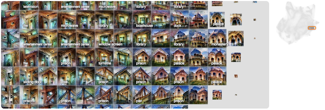
A detail view of an activation atlas from one of the layers of the InceptionV1 vision classification network. It reveals many of the visual detectors that the network uses to classify images, such as different types of fruit-like textures, honeycomb patterns and fabric-like textures.
The activation atlases shown below are built from a convolutional image classification network, Inceptionv1, that was trained on the ImageNet dataset. In general, classification networks are shown an image and then asked to give that image a label from one of 1,000 predetermined classes — such as "carbonara", "snorkel" or "frying pan". To do this, our network evaluates the image data progressively through about ten layers, each made of hundreds of neurons that each activate to varying degrees on different types of image patches. One neuron at one layer might respond positively to a dog's ear, another at an earlier layer might respond to a high-contrast vertical line.

An activation atlas is built by collecting the internal activations from each of these layers of our neural network from one million images. These activations, represented by a complex set of high-dimensional vectors, is projected into useful 2D layouts via UMAP, a dimensionality-reduction technique that preserving some of the local structure of the original high-dimensional space.

This takes care of organizing our activation vectors, but we also need to aggregate them into a more manageable number — all the activations are too many to consume at a glance. To do this, we draw a grid over the 2D layout we created. For each cell in our grid, we average all the activations that lie within the boundaries of that cell, and use feature visualization to create an iconic representation.
Left: A randomized set of one million images is fed through the network, collecting one random spatial activation per image. Center: The activations are fed through UMAP to reduce them to two dimensions. They are then plotted, with similar activations placed near each other. Right: We then draw a grid, average the activations that fall within a cell, and run feature inversion on the averaged activation.
Below we can see an activation atlas for just one layer in a neural network (remember that these classification models can have half a dozen or more layers). It reveals a universe of the visual concepts the network has learned to classify images at this layer. This atlas can be a bit overwhelming at first glance — there's a lot going on! This diversity is a reflection of the variety of visual abstractions and concepts the model has developed.
An overview of an activation atlas for one of the many layers (mixed4c) within Inception v1. It is about halfway through the network.
In this detail, we can see detectors for different types of leaves and plants.
Here we can see different detectors for water, lakes and sandbars.
Here we see different types of buildings and bridges.
As we mentioned before, there are many more layers in this network. Let's look at the layers that came before this one to see how these concepts become more refined as we go deeper into the network (Each layer builds its activations on top of the preceding layer's activations).
In an early layer, mixed4a, there is a vague "mammalian" area.
By the next layer in the network, mixed4b, animals and people have been disentangled, with some fruit and food emerging in the middle.
By layer mixed4c these concepts are further refined and differentiated into small "peninsulas".
Here we've seen the global structure evolve from layer to layer, but each of the individual concepts also become more specific and complex from layer to layer. If we focus on the areas of three layers that contribute to a specific classification, say "cabbage", we can see this clearly.
Left: This early layer is very nonspecific in comparison to the others. Center: By the middle layer, the images definitely resemble leaves, but they could be any type of plant. Right: By the last layer the images are very specific to cabbage, leaves curved into rounded balls.
There is another phenomenon worth noting: not only are concepts being refined as you move from layer to layer, but new concepts seem to be appearing out of combinations of old ones.
You can see how sand and water are distinct concepts in a middle layer, mixed4c (left and center), both with strong attributions to the classification of "sandbar". Contrast this with a later layer (right), mixed5b, where the two ideas seem to be fused into one activation.
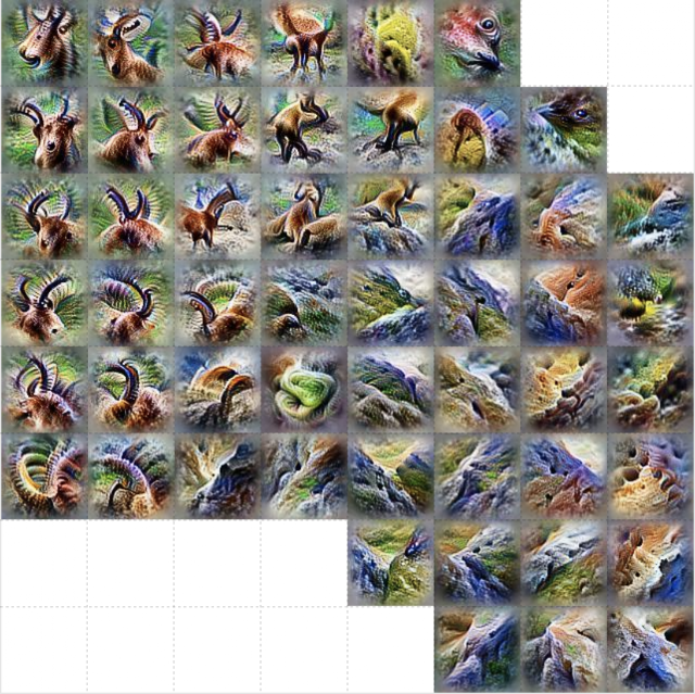
Instead of zooming in on certain areas of the whole atlas for a specific layer, we can also create an atlas at a specific layer for just one of the 1,000 classes in ImageNet. This will show the concepts and detectors that the network most often uses to classify a specific class, say "red fox" for instance.
Here we can more clearly see what the network is focusing on to classify a "red fox". There are pointy ears, white snouts surrounded by red fur, and wooded or snowy backgrounds.
Here we can see the many different scales and angles of detectors for "tile roof".
For "ibex", we see detectors for horns and brown fur, but also environments where we might find such animals, like rocky hillsides.
Like the detectors for tile roof, "artichoke" also has many different sizes of detectors for the texture of an artichoke, but we also get some purple flower detectors. These are presumably detecting the blossoms of an artichoke plant.
These atlases not only reveal nuanced visual abstractions within a model, but they can also reveal high-level misunderstandings. For example, by looking at an activation atlas for a "great white shark" we water and triangular fins (as expected) but we also see something that looks like a baseball. This hints at a shortcut taken by this research model where it conflates the red baseball stitching with the open mouth of a great white shark.
We can test this by using a patch of an image of a baseball to switch the model's classification of a particular image from "grey whale" to "great white shark".
We hope that activation atlases will be a useful tool in the quiver of techniques that are making machine learning more accessible and interpretable. To help you get started, we've released several jupyter notebooks which can be executed immediately in your browser with one click via colab. They build upon the previously released toolkit Lucid, which includes code for many other interpretability visualization techniques included as well. We're excited to see what you discover!

Source: Google AI Blog


Introducing GPipe, an Open Source Library for Efficiently Training Large-scale Neural Network Models


Deep neural networks (DNNs) have advanced many machine learning tasks, including speech recognition, visual recognition, and language processing. Recent advances by BigGan, Bert, and GPT2.0 have shown that ever-larger DNN models lead to better task performance and past progress in visual recognition tasks has also shown a strong correlation between the model size and classification accuracy. For example, the winner of the 2014 ImageNet visual recognition challenge was GoogleNet, which achieved 74.8% top-1 accuracy with 4 million parameters, while just three years later, the winner of the 2017 ImageNet challenge went to Squeeze-and-Excitation Networks, which achieved 82.7% top-1 accuracy with 145.8 million (36x more) parameters. However, in the same period, GPU memory has only increased by a factor of ~3, and the current state-of-the-art image models have already reached the available memory found on Cloud TPUv2s. Hence, there is a strong and pressing need for an efficient, scalable infrastructure that enables large-scale deep learning and overcomes the memory limitation on current accelerators.

Strong correlation between ImageNet accuracy and model size for recently developed representative image classification models
In "GPipe: Efficient Training of Giant Neural Networks using Pipeline Parallelism", we demonstrate the use of pipeline parallelism to scale up DNN training to overcome this limitation. GPipe is a distributed machine learning library that uses synchronous stochastic gradient descent and pipeline parallelism for training, applicable to any DNN that consists of multiple sequential layers. Importantly, GPipe allows researchers to easily deploy more accelerators to train larger models and to scale the performance without tuning hyperparameters. To demonstrate the effectiveness of GPipe, we trained an AmoebaNet-B with 557 million model parameters and input image size of 480 x 480 on Google Cloud TPUv2s. This model performed well on multiple popular datasets, including pushing the single-crop ImageNet accuracy to 84.3%, the CIFAR-10 accuracy to 99%, and the CIFAR-100 accuracy to 91.3%. The core GPipe library has been open sourced under the Lingvo framework.

From Mini- to Micro-Batches
There are two standard ways to speed up moderate-size DNN models. The data parallelism approach employs more machines and splits the input data across them. Another way is to move the model to accelerators, such as GPUs or TPUs, which have special hardware to accelerate model training. However, accelerators have limited memory and limited communication bandwidth with the host machine. Thus, model parallelism is needed for training a bigger DNN model on accelerators by dividing the model into partitions and assigning different partitions to different accelerators. But due to the sequential nature of DNNs, this naive strategy may result in only one accelerator being active during computation, significantly underutilizing accelerator compute capacity. On the other hand, a standard data parallelism approach allows concurrent training of the same model with different input data on multiple accelerators, but cannot increase the maximum model size an accelerator can support.

To enable efficient training across multiple accelerators, GPipe partitions a model across different accelerators and automatically splits a mini-batch of training examples into smaller micro-batches. By pipelining the execution across micro-batches, accelerators can operate in parallel. In addition, gradients are consistently accumulated across micro-batches, so that the number of partitions does not affect the model quality.


Top: The naive model parallelism strategy leads to severe underutilization due to the sequential nature of the network. Only one accelerator is active at a time. Bottom: GPipe divides the input mini-batch into smaller micro-batches, enabling different accelerators to work on separate micro-batches at the same time.
Maximizing Memory and Efficiency
GPipe maximizes memory allocation for model parameters. We ran the experiments on Cloud TPUv2s, each of which has 8 accelerator cores and 64 GB memory (8 GB per accelerator). Without GPipe, a single accelerator can train up to 82 million model parameters due to memory limits. Thanks to recomputation in backpropagation and batch splitting, GPipe reduced intermediate activation memory from 6.26 GB to 3.46GB, enabling 318 million parameters on a single accelerator. We also saw that with pipeline parallelism the maximum model size was proportional to the number of partitions, as expected. With GPipe, AmoebaNet was able to incorporate 1.8 billion parameters on the 8 accelerators of a Cloud TPUv2, 25x times more than is possible without GPipe.

To test efficiency, we measured the effects of GPipe on the model throughput of AmoebaNet-D. Since training required at least two accelerators to fit the model size, we measured the speedup with respect to the naive case with two partitions but no pipeline parallelization. We observed an almost linear speedup in training. Compared to the naive approach with two partitions, distributing the model across four times the accelerators achieved a speedup of 3.5x. While all experiments in our paper used Cloud TPUv2, we see even better performance with the currently available Cloud TPUv3s, each of which has 16 accelerator cores and 256 GB (16 GB per accelerator). GPipe enabled 8 billion parameter Transformer language models on 1024-token sentences with a speedup of 11x when distributing the model across all sixteen accelerators.


Speedup of AmoebaNet-D using GPipe. This model could not fit into one accelerator. The baseline naive-2 is the performance of the native partition approach when the model is split into two partitions. Pipeline-k refers to the performance of GPipe that splits the model into k partitions with k accelerators.
GPipe can also scale training by employing even more accelerators without changes in the hyperparameters. Therefore, it can be combined with data parallelism to scale neural network training using even more accelerators in a complementary way.

Testing Accuracy
We used GPipe to verify the hypothesis that scaling up existing neural networks can achieve even better model quality. We trained an AmoebaNet-B with 557 million model parameters and input image size of 480 x 480 on the ImageNet ILSVRC-2012 dataset. The network was divided into 4 partitions and applied parallel training processes to both model and data. This giant model reached the state-of-the-art 84.3% top-1 / 97% top-5 single-crop validation accuracy without any external data. Large neural networks are not only applicable to datasets like ImageNet, but also relevant for other datasets through transfer learning. It has been shown that better ImageNet models transfer better. We ran transfer learning experiments on the CIFAR10 and CIFAR100 datasets. Our giant models increased the best published CIFAR-10 accuracy to 99% and CIFAR-100 accuracy to 91.3%.

Conclusion
The ongoing development and success of many practical machine learning applications, such as autonomous driving and medical imaging, depend on achieving the highest accuracy possible. As this often requires building larger and even more complex models, we are happy to provide GPipe to the broader research community, and hope it is a useful infrastructure for efficient training of large-scale DNNs.

Acknowledgments
Special thanks to the co-authors of the paper: Youlong Cheng, Dehao Che, HyoukJoong Lee, Jiquan Ngiam, Quoc V. Le, and Zhifeng Chen. We wish to thank Esteban Real, Alok Aggarwal, Xiaodan Song, Naveen Kumar, Mark Heffernan, Rajat Monga, Megan Kacholia, Samy Bengio, and Jeff Dean for their support and valuable input; Noam Shazeer, Patrick Nguyen, Xiaoqiang Zheng, Yonghui Wu, Barret Zoph, Ekin Cubuk, Jonathan Shen, Tianqi Chen, and Vijay Vasudevan for helpful discussions and inspirations; and the larger Google Brain team.

Source: Google AI Blog


Long-Range Robotic Navigation via Automated Reinforcement Learning


In the United States alone, there are 3 million people with a mobility impairment that prevents them from ever leaving their homes. Service robots that can autonomously navigate long distances can improve the independence of people with limited mobility, for example, by bringing them groceries, medicine, and packages. Research has demonstrated that deep reinforcement learning (RL) is good at mapping raw sensory input to actions, e.g. learning to grasp objects and for robot locomotion, but RL agents usually lack the understanding of large physical spaces needed to safely navigate long distances without human help and to easily adapt to new spaces.

In three recent papers, “Learning Navigation Behaviors End-to-End with AutoRL,” “PRM-RL: Long-Range Robotic Navigation Tasks by Combining Reinforcement Learning and Sampling-based Planning”, and “Long-Range Indoor Navigation with PRM-RL”, we investigate easy-to-adapt robotic autonomy by combining deep RL with long-range planning. We train local planner agents to perform basic navigation behaviors, traversing short distances safely without collisions with moving obstacles. The local planners take noisy sensor observations, such as a 1D lidar that provides distances to obstacles, and output linear and angular velocities for robot control. We train the local planner in simulation with AutoRL, a method that automates the search for RL reward and neural network architecture. Despite their limited range of 10 - 15 meters, the local planners transfer well to both real robots and to new, previously unseen environments. This enables us to use them as building blocks for navigation in large spaces. We then build a roadmap, a graph where nodes are locations and edges connect the nodes only if local planners, which mimic real robots well with their noisy sensors and control, can traverse between them reliably.

Automating Reinforcement Learning (AutoRL)
In our first paper, we train the local planners in small, static environments. However, training with standard deep RL algorithms, such as Deep Deterministic Policy Gradient (DDPG), poses several challenges. For example, the true objective of the local planners is to reach the goal, which represents a sparse reward. In practice, this requires researchers to spend significant time iterating and hand-tuning the rewards. Researchers must also make decisions about the neural network architecture, without clear accepted best practices. And finally, algorithms like DDPG are unstable learners and often exhibit catastrophic forgetfulness.

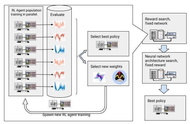
To overcome those challenges, we automate the deep Reinforcement Learning (RL) training. AutoRL is an evolutionary automation layer around deep RL that searches for a reward and neural network architecture using large-scale hyperparameter optimization. It works in two phases, reward search and neural network architecture search. During the reward search, AutoRL trains a population of DDPG agents concurrently over several generations, each with a slightly different reward function optimizing for the local planner’s true objective: reaching the destination. At the end of the reward search phase, we select the reward that leads the agents to its destination most often. In the neural network architecture search phase, we repeat the process, this time using the selected reward and tuning the network layers, optimizing for the cumulative reward.
Automating reinforcement learning with reward and neural network architecture search.
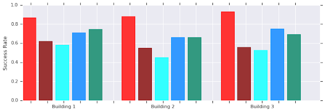
However, this iterative process means AutoRL is not sample efficient. Training one agent takes 5 million samples; AutoRL training over 10 generations of 100 agents requires 5 billion samples - equivalent to 32 years of training! The benefit is that after AutoRL the manual training process is automated, and DDPG does not experience catastrophic forgetfulness. Most importantly, the resulting policies are higher quality — AutoRL policies are robust to sensor, actuator and localization noise, and generalize well to new environments. Our best policy is 26% more successful than other navigation methods across our test environments.
AutoRL (red) success over short distances (up to 10 meters) in several unseen buildings. Compared to hand-tuned DDPG (dark-red), artificial potential fields (light blue), dynamic window approach (blue), and behavior cloning (green).
AutoRL local planner policy transfer to robots in real, unstructured environments
While these policies only perform local navigation, they are robust to moving obstacles and transfer well to real robots, even in unstructured environments. Though they were trained in simulation with only static obstacles, they can also handle moving objects effectively. The next step is to combine the AutoRL policies with sampling-based planning to extend their reach and enable long-range navigation.

Achieving Long Range Navigation with PRM-RL
Sampling-based planners tackle long-range navigation by approximating robot motions. For example, probabilistic roadmaps (PRMs) sample robot poses and connect them with feasible transitions, creating roadmaps that capture valid movements of a robot across large spaces. In our second paper, which won Best Paper in Service Robotics at ICRA 2018, we combine PRMs with hand-tuned RL-based local planners (without AutoRL) to train robots once locally and then adapt them to different environments.

First, for each robot we train a local planner policy in a generic simulated training environment. Next, we build a PRM with respect to that policy, called a PRM-RL, over a floor plan for the deployment environment. The same floor plan can be used for any robot we wish to deploy in the building in a one time per robot+environment setup.

To build a PRM-RL we connect sampled nodes only if the RL-based local planner, which represents robot noise well, can reliably and consistently navigate between them. This is done via Monte Carlo simulation. The resulting roadmap is tuned to both the abilities and geometry of the particular robot. Roadmaps for robots with the same geometry but different sensors and actuators will have different connectivity. Since the agent can navigate around corners, nodes without clear line of sight can be included. Whereas nodes near walls and obstacles are less likely to be connected into the roadmap because of sensor noise. At execution time, the RL agent navigates from roadmap waypoint to waypoint.
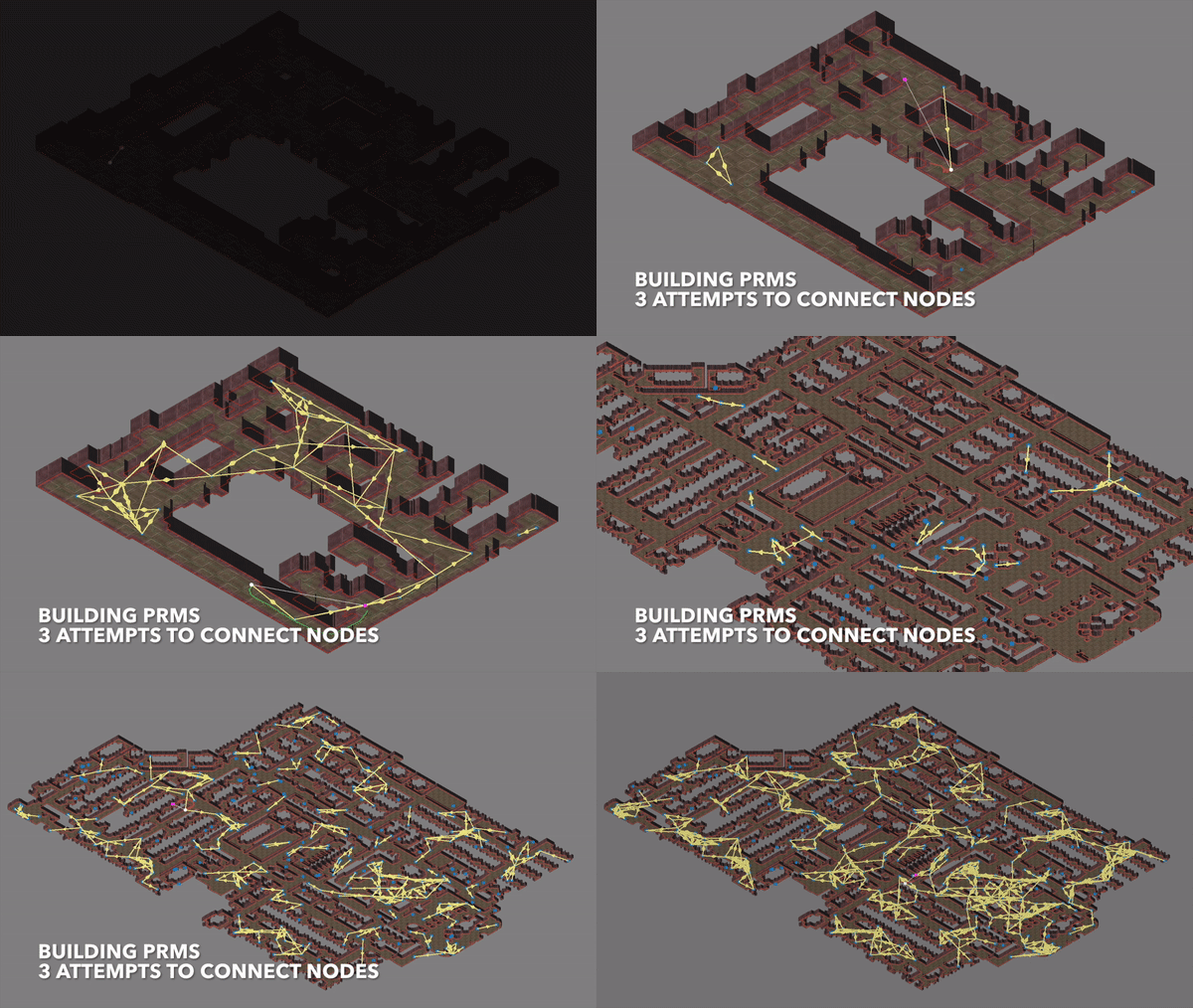
Roadmap being built with 3 Monte Carlo simulations per randomly selected node pair.
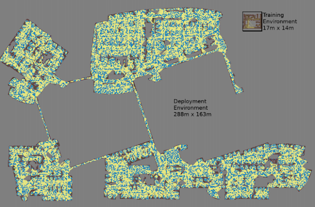
The largest map was 288 meters by 163 meters and contains almost 700,000 edges, collected over 4 days using 300 workers in a cluster requiring 1.1 billion collision checks.
The third paper makes several improvements over the original PRM-RL. First, we replace the hand-tuned DDPG with AutoRL-trained local planners, which results in improved long-range navigation. Second, it adds Simultaneous Localization and Mapping (SLAM) maps, which robots use at execution time, as a source for building the roadmaps. Because SLAM maps are noisy, this change closes the “sim2real gap”, a phonomena in robotics where simulation-trained agents significantly underperform when transferred to real-robots. Our simulated success rates are the same as in on-robot experiments. Last, we added distributed roadmap building, resulting in very large scale roadmaps containing up to 700,000 nodes.

We evaluated the method using our AutoRL agent, building roadmaps using the floor maps of offices up to 200x larger than the training environments, accepting edges with at least 90% success over 20 trials. We compared PRM-RL to a variety of different methods over distances up to 100m, well beyond the local planner range. PRM-RL had 2 to 3 times the rate of success over baseline because the nodes were connected appropriately for the robot’s capabilities.
Navigation over 100 meters success rates in several buildings. First paper -AutoRL local planner only (blue); original PRMs (red); path-guided artificial potential fields (yellow); second paper (green); third paper - PRMs with AutoRL (orange).
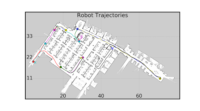
We tested PRM-RL on multiple real robots and real building sites. One set of tests are shown below; the robot is very robust except near cluttered areas and off the edge of the SLAM map.
On-robot experiments
Conclusion
Autonomous robot navigation can significantly improve independence of people with limited mobility. We can achieve this by development of easy-to-adapt robotic autonomy, including methods that can be deployed in new environments using information that it is already available. This is done by automating the learning of basic, short-range navigation behaviors with AutoRL and using these learned policies in conjunction with SLAM maps to build roadmaps. These roadmaps consist of nodes connected by edges that robots can traverse consistently. The result is a policy that once trained can be used across different environments and can produce a roadmap custom-tailored to the particular robot.

Acknowledgements
The research was done by, in alphabetical order, Hao-Tien Lewis Chiang, James Davidson, Aleksandra Faust, Marek Fiser, Anthony Francis, Jasmine Hsu, J. Chase Kew, Tsang-Wei Edward Lee, Ken Oslund, Oscar Ramirez from Robotics at Google and Lydia Tapia from University of New Mexico. We thank Alexander Toshev, Brian Ichter, Chris Harris, and Vincent Vanhoucke for helpful discussions.

Source: Google AI Blog


Learning to Generalize from Sparse and Underspecified Rewards


Reinforcement learning (RL) presents a unified and flexible framework for optimizing goal-oriented behavior, and has enabled remarkable success in addressing challenging tasks such as playing video games, continuous control, and robotic learning. The success of RL algorithms in these application domains often hinges on the availability of high-quality and dense reward feedback. However, broadening the applicability of RL algorithms to environments with sparse and underspecified rewards is an ongoing challenge, requiring a learning agent to generalize (i.e., learn the right behavior) from limited feedback. A natural way to investigate the performance of RL algorithms in such problem settings is via language understanding tasks, where an agent is provided with a natural language input and needs to generate a complex response to achieve a goal specified in the input, while only receiving binary success-failure feedback.

For instance, consider a "blind" agent tasked with reaching a goal position in a maze by following a sequence of natural language commands (e.g., "Right, Up, Up, Right"). Given the input text, the agent (green circle) needs to interpret the commands and take actions based on such interpretation to generate an action sequence (a). The agent receives a reward of 1 if it reaches the goal (red star) and 0 otherwise. Because the agent doesn't have access to any visual information, the only way for the agent to solve this task and generalize to novel instructions is by correctly interpreting the instructions.
In this instruction-following task, the action trajectories a1, a2 and a3 reach the goal, but the sequences a2 and a3 do not follow the instructions. This illustrates the issue of underspecified rewards.
In these tasks, the RL agent needs to learn to generalize from sparse (only a few trajectories lead to a non-zero reward) and underspecified (no distinction between purposeful and accidental success) rewards. Importantly, because of underspecified rewards, the agent may receive positive feedback for exploiting spurious patterns in the environment. This can lead to reward hacking, causing unintended and harmful behavior when deployed in real-world systems.

In "Learning to Generalize from Sparse and Underspecified Rewards", we address the issue of underspecified rewards by developing Meta Reward Learning (MeRL), which provides more refined feedback to the agent by optimizing an auxiliary reward function. MeRL is combined with a memory buffer of successful trajectories collected using a novel exploration strategy to learn from sparse rewards. The effectiveness of our approach is demonstrated on semantic parsing, where the goal is to learn a mapping from natural language to logical forms (e.g., mapping questions to SQL programs). In the paper, we investigate the weakly-supervised problem setting, where the goal is to automatically discover logical programs from question-answer pairs, without any form of program supervision. For instance, given the question "Which nation won the most silver medals?" and a relevant Wikipedia table, an agent needs to generate an SQL-like program that results in the correct answer (i.e., "Nigeria").
The proposed approach achieves state-of-the-art results on the WikiTableQuestions and WikiSQL benchmarks, improving upon prior work by 1.2% and 2.4% respectively. MeRL automatically learns the auxiliary reward function without using any expert demonstrations, (e.g., ground-truth programs) making it more widely applicable and distinct from previous reward learning approaches. The diagram below depicts a high level overview of our approach:
Overview of the proposed approach. We employ (1) mode covering exploration to collect a diverse set of successful trajectories in a memory buffer; (2) Meta-learning or Bayesian optimization to learn an auxiliary reward that provides more refined feedback for policy optimization.
Meta Reward Learning (MeRL)
The key insight of MeRL in dealing with underspecified rewards is that spurious trajectories and programs that achieve accidental success are detrimental to the agent's generalization performance. For example, an agent might be able to solve a specific instance of the maze problem above. However, if it learns to perform spurious actions during training, it is likely to fail when provided with unseen instructions. To mitigate this issue, MeRL optimizes a more refined auxiliary reward function, which can differentiate between accidental and purposeful success based on features of action trajectories. The auxiliary reward is optimized by maximizing the trained agent's performance on a hold-out validation set via meta learning.
Schematic illustration of MeRL: The RL agent is trained via the reward signal obtained from the auxiliary reward model while the auxiliary rewards are trained using the generalization error of the agent.
Learning from Sparse Rewards
To learn from sparse rewards, effective exploration is critical to find a set of successful trajectories. Our paper addresses this challenge by utilizing the two directions of Kullback–Leibler (KL) divergence, a measure on how different two probability distributions are. In the example below, we use KL divergence to minimize the difference between a fixed bimodal (shaded purple) and a learned gaussian (shaded green) distribution, which can represent the distribution of the agent's optimal policy and our learned policy respectively. One direction of the KL objective learns a distribution which tries to cover both the modes while the distribution learned by other objective seeks a particular mode (i.e. it prefers one mode over another). Our method exploits the mode covering KL's tendency to focus on multiple peaks to collect a diverse set of successful trajectories and mode seeking KL's implicit preference between trajectories to learn a robust policy.
Left: Optimizing mode covering KL. Right: Optimizing mode seeking KL

Conclusion
Designing reward functions that distinguish between optimal and suboptimal behavior is critical for applying RL to real-world applications. This research takes a small step in the direction of modelling reward functions without any human supervision. In future work, we'd like to tackle the credit-assignment problem in RL from the perspective of automatically learning a dense reward function.

Acknowledgements
This research was done in collaboration with Chen Liang and Dale Schuurmans. We thank Chelsea Finn and Kelvin Guu for their review of the paper.

Source: Google AI Blog


On the Path to Cryogenic Control of Quantum Processors


Building a quantum computer that can solve practical problems that would otherwise be classically intractable due to the computation complexity, cost, energy consumption or time to solution, is the longstanding goal of the Google AI Quantum team. Current thresholds suggest a first generation error-corrected quantum computer will require on the order of 1 million physical qubits, which is more than four orders of magnitude more qubits than exist in Bristlecone, our 72 qubit quantum processor. Increasing the number of physical qubits needed for a fault-tolerant quantum computer while maintaining high-quality control of each qubit are intertwined and exciting technological challenges that will require inventions beyond simply copying and pasting our current control architecture. One critical challenge is reducing the number of input/output control lines per qubit by relocating the room temperature analog control electronics to the 3 kelvin stage in the cryostat, while maintaining high-quality qubit control.

As a step towards solving that challenge, this week we presented our first generation cryogenic-CMOS single-qubit controller at the International Solid State Circuits Conference in San Francisco. Fabricated using commercial CMOS technology, our controller operates at 3 kelvin, consumes less than 2 milliwatts of power and measures just 1 mm by 1.6 mm. Functionally, it provides an instruction set for single-qubit gate operations, providing analog control of a qubit via digital lines between room temperature and 3 kelvin, all while consuming ~1000 times less power compared to our current room temperature control electronics.
Google’s first generation cryogenic-CMOS single-qubit controller (center and zoomed on the right) packaged and ready to be deployed inside our cryostat. The controller measures 1mm by 1.6mm.
How to Control 72 Qubits
In our lab in Santa Barbara, we run programs on Bristlecone by applying gigahertz frequency analog control signals to each of the qubits to manipulate the qubit state, to entangle qubits and to measure the outcomes of our computations. How well we define the shape and frequency of these control signals directly impacts the quality of our computation. To make high-quality qubit control signals, we leverage technology developed for smartphones packaged in server racks at room temperature. Individual coaxial cables deliver these signals to each qubit, which are themselves kept inside a cryostat chilled to 10 millikelvin. While this approach makes sense for a Bristlecone-scale quantum processor, which demands 2 control lines per qubit for 144 unique control signals, we realized that a more integrated approach would be required in order to scale our systems to the million qubit level.
Research Scientist Amit Vainsencher checking the wiring on Bristlecone in one of Google's flagship cryostats. Blue coaxial cables are connected from custom analog control electronics (server rack on the right) to the quantum processor.
In our current setup, the number of physical wires connected from room temperature to the qubits inside the cryostat and the finite cooling power of the cryostat represent a significant constraint. One way to alleviate this is to move the digital to analog control closer to the quantum processor. Currently, our room temperature digital-to-analog waveform generators used to control individual qubits, dissipate ~1 watt of waste heat per qubit. The cooling power of our cryostat at 3 kelvin is 0.1 watt. That means if we crammed 150 waveform generators into our cryostat (never mind the limited physical space inside the refrigerator for a moment) we would overwhelm the cooling power of our cryostat by 1500x, thereby cooking our cryostat and rendering our qubits useless. Therefore, simply installing our existing digital-to-analog control in the cryostat will not set us on the path to control millions of qubits. It is clear we need an integrated low-power qubit control solution.

A Cool Idea
In collaboration with University of Massachusetts Professor Joseph Bardin, we set out to develop custom integrated circuits (ICs) to control our qubits from within the cryostat to ultimately reduce the physical I/O connections to and from our future quantum processors. These ICs would be designed to operate in the ultracold environment, specifically 3 kelvin, and turn digital instructions into analog control pulses for qubits. A key research objective was to first design a custom IC with low power requirements, in order to prevent warming up the cryostat.

We designed our IC to dissipate no more than 2 milliwatts of power at 3 kelvin, which can be challenging as most physical CMOS models assume operation closer to 300 kelvin. After design and fabrication of the IC with the low power design constraints in mind, we verified that the cryogenic-CMOS qubit controller worked at room temperature. We then mounted it in our cryostat at 3 kelvin and connected it to a qubit (mounted at 10 millikelvin in the same cryostat). We carried out a series of experiments to establish that the cryogenic-CMOS qubit controller worked as designed, and most importantly, that we hadn't just installed a heater inside our cryostat.
Schematic of the cryogenic-CMOS qubit controller mounted on the 3 kelvin stage of our dilution refrigerator and connected to a qubit. Our standard qubit control electronics were connected in parallel to enable control and measurement of the qubit as an in-situ check experiment.
Performance at Low Temperature
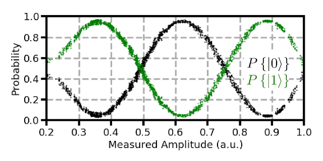
Baseline experiments for our new quantum control hardware, including T1, Rabi oscillations, and single qubit gates, show similar performance compared to our standard room-temperature qubit control electronics: qubit coherence time was virtually unchanged, and high-visibility Rabi oscillations were observed by varying the amplitude of the pulses out of the cryogenic-CMOS qubit controller—a signature response of a driven qubit.

Comparison of the qubit coherence time measured using the standard and cryogenic quantum controllers.
Measured Rabi amplitude oscillations using the cryogenic controller. The green and black traces are the probability of measuring the qubits in the 1 and 0 states, respectively.
Next Steps
Although all of these results are promising, this first generation cryogenic-CMOS qubit controller is but one small step towards a truly scalable qubit control and measurement system. For instance, our controller is only able to address a single qubit, and it still requires several connections to room temperature. In addition, we still need to work hard to quantify the error rates for single qubit gates. As such, we are excited to reduce the energy required to control qubits and still maintain the delicate control required to perform high-quality qubit operations.

Acknowledgements
This work was carried out with the support of the Google Visiting Researcher Program while Prof. Bardin, an Associate Professor with the University of Massachusetts Amherst, was on sabbatical with the Google AI Quantum Team. This work would not have been possible without the many contributions of members of the Google AI Quantum team, especially Evan Jeffrey for his integration of the cryo-CMOS controller into the qubit calibration software, Ted White for his on-demand qubit calibrations and Trent Huang for his tireless design rules checks.

Source: Google AI Blog


Introducing PlaNet: A Deep Planning Network for Reinforcement Learning


Research into how artificial agents can improve their decisions over time is progressing rapidly via reinforcement learning (RL). For this technique, an agent observes a stream of sensory inputs (e.g. camera images) while choosing actions (e.g. motor commands), and sometimes receives a reward for achieving a specified goal. Model-free approaches to RL aim to directly predict good actions from the sensory observations, enabling DeepMind's DQN to play Atari and other agents to control robots. However, this blackbox approach often requires several weeks of simulated interaction to learn through trial and error, limiting its usefulness in practice.

Model-based RL, in contrast, attempts to have agents learn how the world behaves in general. Instead of directly mapping observations to actions, this allows an agent to explicitly plan ahead, to more carefully select actions by "imagining" their long-term outcomes. Model-based approaches have achieved substantial successes, including AlphaGo, which imagines taking sequences of moves on a fictitious board with the known rules of the game. However, to leverage planning in unknown environments (such as controlling a robot given only pixels as input), the agent must learn the rules or dynamics from experience. Because such dynamics models in principle allow for higher efficiency and natural multi-task learning, creating models that are accurate enough for successful planning is a long-standing goal of RL.

To spur progress on this research challenge and in collaboration with DeepMind, we present the Deep Planning Network (PlaNet) agent, which learns a world model from image inputs only and successfully leverages it for planning. PlaNet solves a variety of image-based control tasks, competing with advanced model-free agents in terms of final performance while being 5000% more data efficient on average. We are additionally releasing the source code for the research community to build upon.
The PlaNet agent learning to solve a variety of continuous control tasks from images in 2000 attempts. Previous agents that do not learn a model of the environment often require 50 times as many attempts to reach comparable performance.
How PlaNet Works
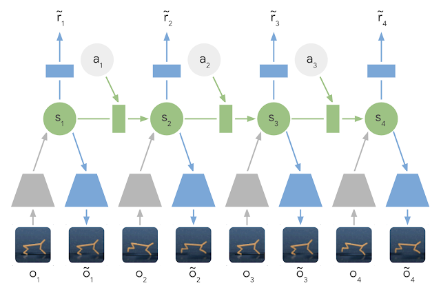
In short, PlaNet learns a dynamics model given image inputs and efficiently plans with it to gather new experience. In contrast to previous methods that plan over images, we rely on a compact sequence of hidden or latent states. This is called a latent dynamics model: instead of directly predicting from one image to the next image, we predict the latent state forward. The image and reward at each step is then generated from the corresponding latent state. By compressing the images in this way, the agent can automatically learn more abstract representations, such as positions and velocities of objects, making it easier to predict forward without having to generate images along the way.
Learned Latent Dynamics Model: In a latent dynamics model, the information of the input images is integrated into the hidden states (green) using the encoder network (grey trapezoids). The hidden state is then projected forward in time to predict future images (blue trapezoids) and rewards (blue rectangle).
To learn an accurate latent dynamics model, we introduce:
  • A Recurrent State Space Model: A latent dynamics model with both deterministic and stochastic components, allowing to predict a variety of possible futures as needed for robust planning, while remembering information over many time steps. Our experiments indicate both components to be crucial for high planning performance.
  • A Latent Overshooting Objective: We generalize the standard training objective for latent dynamics models to train multi-step predictions, by enforcing consistency between one-step and multi-step predictions in latent space. This yields a fast and effective objective that improves long-term predictions and is compatible with any latent sequence model.
While predicting future images allows us teach the model, encoding and decoding images (trapezoids in the figure above) requires significant computation, which would slow down planning. However, planning in the compact latent state space is fast since we only need to predict future rewards, and not images, to evaluate an action sequence. For example, the agent can imagine how the position of a ball and its distance to the goal will change for certain actions, without having to visualize the scenario. This allows us to compare 10,000 imagined action sequences with a large batch size every time the agent chooses an action. We then execute the first action of the best sequence found and replan at the next step.
Planning in Latent Space: For planning, we encode past images (gray trapezoid) into the current hidden state (green). From there, we efficiently predict future rewards for multiple action sequences. Note how the expensive image decoder (blue trapezoid) from the previous figure is gone. We then execute the first action of the best sequence found (red box).
Compared to our preceding work on world models, PlaNet works without a policy network -- it chooses actions purely by planning, so it benefits from model improvements on the spot. For the technical details, check out our online research paper or the PDF version.

PlaNet vs. Model-Free Methods
We evaluate PlaNet on continuous control tasks. The agent is only given image observations and rewards. We consider tasks that pose a variety of different challenges:
  • A cartpole swing-up task, with a fixed camera, so the cart can move out of sight. The agent thus must absorb and remember information over multiple frames.
  • A finger spin task that requires predicting two separate objects, as well as the interactions between them.
  • A cheetah running task that includes contacts with the ground that are difficult to predict precisely, calling for a model that can predict multiple possible futures.
  • A cup task, which only provides a sparse reward signal once a ball is caught. This demands accurate predictions far into the future to plan a precise sequence of actions.
  • A walker task, in which a simulated robot starts off by lying on the ground, and must first learn to stand up and then walk.
PlaNet agents trained on a variety of image-based control tasks. The animation shows the input images as the agent is solving the tasks. The tasks pose different challenges: partial observability, contacts with the ground, sparse rewards for catching a ball, and controlling a challenging bipedal robot.
Our work constitutes one of the first examples where planning with a learned model outperforms model-free methods on image-based tasks. The table below compares PlaNet to the well-known A3C agent and the D4PG agent, that combines recent advances in model-free RL. The numbers for these baselines are taken from the DeepMind Control Suite. PlaNet clearly outperforms A3C on all tasks and reaches final performance close to D4PG while, using 5000% less interaction with the environment on average.
One Agent for All Tasks
Additionally, we train a single PlaNet agent to solve all six tasks. The agent is randomly placed into different environments without knowing the task, so it needs to infer the task from its image observations. Without changes to the hyper parameters, the multi-task agent achieves the same mean performance as individual agents. While learning slower on the cartpole tasks, it learns substantially faster and reaches a higher final performance on the challenging walker task that requires exploration.
Video predictions of the PlaNet agent trained on multiple tasks. Holdout episodes collected with the trained agent are shown above and open-loop agent hallucinations below. The agent observes the first 5 frames as context to infer the task and state and accurately predicts ahead for 50 steps given a sequence of actions.
Conclusion
Our results showcase the promise of learning dynamics models for building autonomous RL agents. We advocate for further research that focuses on learning accurate dynamics models on tasks of even higher difficulty, such as 3D environments and real-world robotics tasks. A possible ingredient for scaling up is the processing power of TPUs. We are excited about the possibilities that model-based reinforcement learning opens up, including multi-task learning, hierarchical planning and active exploration using uncertainty estimates.

Acknowledgements
This project is a collaboration with Timothy Lillicrap, Ian Fischer, Ruben Villegas, Honglak Lee, David Ha and James Davidson. We further thank everybody who commented on our paper draft and provided feedback at any point throughout the project.


Source: Google AI Blog