Tag Archives: Self-Supervised Learning

ScreenAI: A visual language model for UI and visually-situated language understanding

Screen user interfaces (UIs) and infographics, such as charts, diagrams and tables, play important roles in human communication and human-machine interaction as they facilitate rich and interactive user experiences. UIs and infographics share similar design principles and visual language (e.g., icons and layouts), that offer an opportunity to build a single model that can understand, reason, and interact with these interfaces. However, because of their complexity and varied presentation formats, infographics and UIs present a unique modeling challenge.

To that end, we introduce “ScreenAI: A Vision-Language Model for UI and Infographics Understanding”. ScreenAI improves upon the PaLI architecture with the flexible patching strategy from pix2struct. We train ScreenAI on a unique mixture of datasets and tasks, including a novel Screen Annotation task that requires the model to identify UI element information (i.e., type, location and description) on a screen. These text annotations provide large language models (LLMs) with screen descriptions, enabling them to automatically generate question-answering (QA), UI navigation, and summarization training datasets at scale. At only 5B parameters, ScreenAI achieves state-of-the-art results on UI- and infographic-based tasks (WebSRC and MoTIF), and best-in-class performance on Chart QA, DocVQA, and InfographicVQA compared to models of similar size. We are also releasing three new datasets: Screen Annotation to evaluate the layout understanding capability of the model, as well as ScreenQA Short and Complex ScreenQA for a more comprehensive evaluation of its QA capability.


ScreenAI

ScreenAI’s architecture is based on PaLI, composed of a multimodal encoder block and an autoregressive decoder. The PaLI encoder uses a vision transformer (ViT) that creates image embeddings and a multimodal encoder that takes the concatenation of the image and text embeddings as input. This flexible architecture allows ScreenAI to solve vision tasks that can be recast as text+image-to-text problems.

On top of the PaLI architecture, we employ a flexible patching strategy introduced in pix2struct. Instead of using a fixed-grid pattern, the grid dimensions are selected such that they preserve the native aspect ratio of the input image. This enables ScreenAI to work well across images of various aspect ratios.

The ScreenAI model is trained in two stages: a pre-training stage followed by a fine-tuning stage. First, self-supervised learning is applied to automatically generate data labels, which are then used to train ViT and the language model. ViT is frozen during the fine-tuning stage, where most data used is manually labeled by human raters.

ScreenAI model architecture.


Data generation

To create a pre-training dataset for ScreenAI, we first compile an extensive collection of screenshots from various devices, including desktops, mobile, and tablets. This is achieved by using publicly accessible web pages and following the programmatic exploration approach used for the RICO dataset for mobile apps. We then apply a layout annotator, based on the DETR model, that identifies and labels a wide range of UI elements (e.g., image, pictogram, button, text) and their spatial relationships. Pictograms undergo further analysis using an icon classifier capable of distinguishing 77 different icon types. This detailed classification is essential for interpreting the subtle information conveyed through icons. For icons that are not covered by the classifier, and for infographics and images, we use the PaLI image captioning model to generate descriptive captions that provide contextual information. We also apply an optical character recognition (OCR) engine to extract and annotate textual content on screen. We combine the OCR text with the previous annotations to create a detailed description of each screen.

A mobile app screenshot with generated annotations that include UI elements and their descriptions, e.g., TEXT elements also contain the text content from OCR, IMAGE elements contain image captions, LIST_ITEMs contain all their child elements.


LLM-based data generation

We enhance the pre-training data's diversity using PaLM 2 to generate input-output pairs in a two-step process. First, screen annotations are generated using the technique outlined above, then we craft a prompt around this schema for the LLM to create synthetic data. This process requires prompt engineering and iterative refinement to find an effective prompt. We assess the generated data's quality through human validation against a quality threshold.


You only speak JSON. Do not write text that isn’t JSON.
You are given the following mobile screenshot, described in words. Can you generate 5 questions regarding the content of the screenshot as well as the corresponding short answers to them? 

The answer should be as short as possible, containing only the necessary information. Your answer should be structured as follows:
questions: [
{{question: the question,
    answer: the answer
}},
 ...
]

{THE SCREEN SCHEMA}

A sample prompt for QA data generation.

By combining the natural language capabilities of LLMs with a structured schema, we simulate a wide range of user interactions and scenarios to generate synthetic, realistic tasks. In particular, we generate three categories of tasks:

  • Question answering: The model is asked to answer questions regarding the content of the screenshots, e.g., “When does the restaurant open?”
  • Screen navigation: The model is asked to convert a natural language utterance into an executable action on a screen, e.g., “Click the search button.”
  • Screen summarization: The model is asked to summarize the screen content in one or two sentences.
Block diagram of our workflow for generating data for QA, summarization and navigation tasks using existing ScreenAI models and LLMs. Each task uses a custom prompt to emphasize desired aspects, like questions related to counting, involving reasoning, etc.

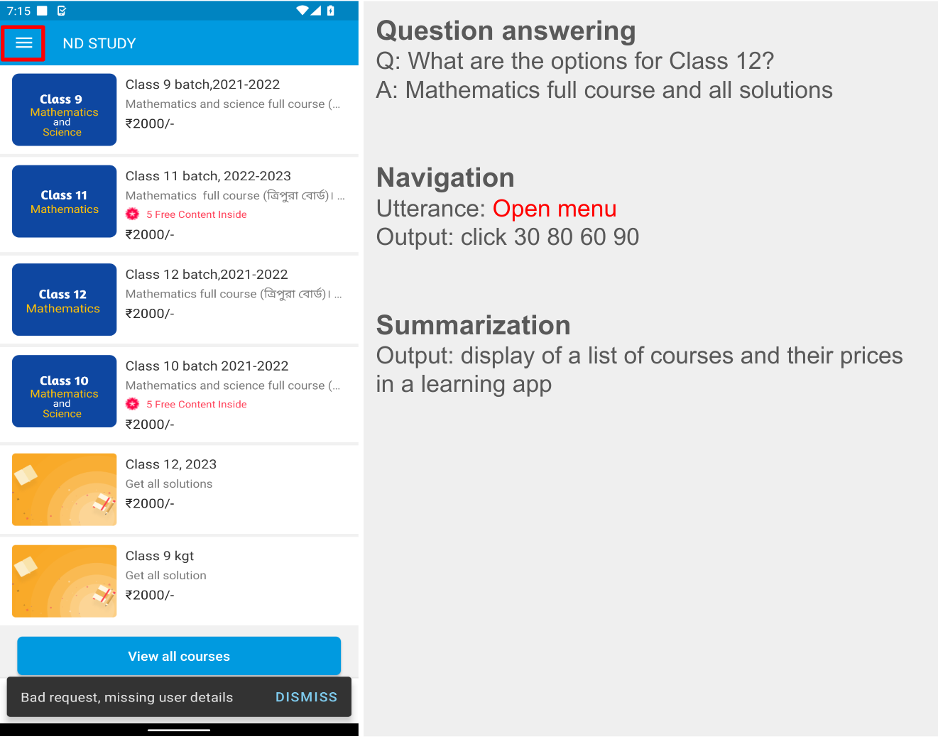
LLM-generated data. Examples for screen QA, navigation and summarization. For navigation, the action bounding box is displayed in red on the screenshot.


Experiments and results

As previously mentioned, ScreenAI is trained in two stages: pre-training and fine-tuning. Pre-training data labels are obtained using self-supervised learning and fine-tuning data labels comes from human raters.

We fine-tune ScreenAI using public QA, summarization, and navigation datasets and a variety of tasks related to UIs. For QA, we use well established benchmarks in the multimodal and document understanding field, such as ChartQA, DocVQA, Multi page DocVQA, InfographicVQA, OCR VQA, Web SRC and ScreenQA. For navigation, datasets used include Referring Expressions, MoTIF, Mug, and Android in the Wild. Finally, we use Screen2Words for screen summarization and Widget Captioning for describing specific UI elements. Along with the fine-tuning datasets, we evaluate the fine-tuned ScreenAI model using three novel benchmarks:

  1. Screen Annotation: Enables the evaluation model layout annotations and spatial understanding capabilities.
  2. ScreenQA Short: A variation of ScreenQA, where its ground truth answers have been shortened to contain only the relevant information that better aligns with other QA tasks.
  3. Complex ScreenQA: Complements ScreenQA Short with more difficult questions (counting, arithmetic, comparison, and non-answerable questions) and contains screens with various aspect ratios.

The fine-tuned ScreenAI model achieves state-of-the-art results on various UI and infographic-based tasks (WebSRC and MoTIF) and best-in-class performance on Chart QA, DocVQA, and InfographicVQA compared to models of similar size. ScreenAI achieves competitive performance on Screen2Words and OCR-VQA. Additionally, we report results on the new benchmark datasets introduced to serve as a baseline for further research.

Comparing model performance of ScreenAI with state-of-the-art (SOTA) models of similar size.

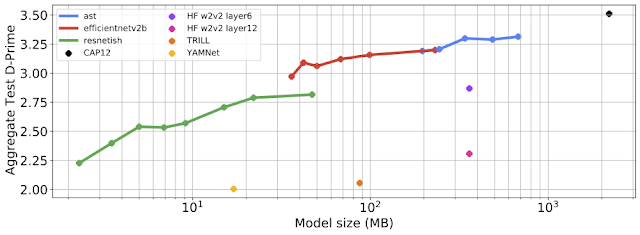
Next, we examine ScreenAI’s scaling capabilities and observe that across all tasks, increasing the model size improves performances and the improvements have not saturated at the largest size.

Model performance increases with size, and the performance has not saturated even at the largest size of 5B params.


Conclusion

We introduce the ScreenAI model along with a unified representation that enables us to develop self-supervised learning tasks leveraging data from all these domains. We also illustrate the impact of data generation using LLMs and investigate improving model performance on specific aspects with modifying the training mixture. We apply all of these techniques to build multi-task trained models that perform competitively with state-of-the-art approaches on a number of public benchmarks. However, we also note that our approach still lags behind large models and further research is needed to bridge this gap.


Acknowledgements

This project is the result of joint work with Maria Wang, Fedir Zubach, Hassan Mansoor, Vincent Etter, Victor Carbune, Jason Lin, Jindong Chen and Abhanshu Sharma. We thank Fangyu Liu, Xi Chen, Efi Kokiopoulou, Jesse Berent, Gabriel Barcik, Lukas Zilka, Oriana Riva, Gang Li,Yang Li, Radu Soricut, and Tania Bedrax-Weiss for their insightful feedback and discussions, along with Rahul Aralikatte, Hao Cheng and Daniel Kim for their support in data preparation. We also thank Jay Yagnik, Blaise Aguera y Arcas, Ewa Dominowska, David Petrou, and Matt Sharifi for their leadership, vision and support. We are very grateful toTom Small for helping us create the animation in this post.

Source: Google AI Blog


SimPer: Simple self-supervised learning of periodic targets

Learning from periodic data (signals that repeat, such as a heart beat or the daily temperature changes on Earth’s surface) is crucial for many real-world applications, from monitoring weather systems to detecting vital signs. For example, in the environmental remote sensing domain, periodic learning is often needed to enable nowcasting of environmental changes, such as precipitation patterns or land surface temperature. In the health domain, learning from video measurement has shown to extract (quasi-)periodic vital signs such as atrial fibrillation and sleep apnea episodes.

Approaches like RepNet highlight the importance of these types of tasks, and present a solution that recognizes repetitive activities within a single video. However, these are supervised approaches that require a significant amount of data to capture repetitive activities, all labeled to indicate the number of times an action was repeated. Labeling such data is often challenging and resource-intensive, requiring researchers to manually capture gold-standard temporal measurements that are synchronized with the modality of interest (e.g., video or satellite imagery).

Alternatively, self-supervised learning (SSL) methods (e.g., SimCLR and MoCo v2), which leverage a large amount of unlabeled data to learn representations that capture periodic or quasi-periodic temporal dynamics, have demonstrated success in solving classification tasks. However, they overlook the intrinsic periodicity (i.e., the ability to identify if a frame is part of a periodic process) in data and fail to learn robust representations that capture periodic or frequency attributes. This is because periodic learning exhibits characteristics that are distinct from prevailing learning tasks.

Feature similarity is different in the context of periodic representations as compared to static features (e.g., images). For example, videos that are offset by short time delays or are reversed should be similar to the original sample, whereas videos that have been upsampled or downsampled by a factor x should be different from the original sample by a factor of x.

To address these challenges, in “SimPer: Simple Self-Supervised Learning of Periodic Targets”, published at the eleventh International Conference on Learning Representations (ICLR 2023), we introduced a self-supervised contrastive framework for learning periodic information in data. Specifically, SimPer leverages the temporal properties of periodic targets using temporal self-contrastive learning, where positive and negative samples are obtained through periodicity-invariant and periodicity-variant augmentations from the same input instance. We propose periodic feature similarity that explicitly defines how to measure similarity in the context of periodic learning. Moreover, we design a generalized contrastive loss that extends the classic InfoNCE loss to a soft regression variant that enables contrasting over continuous labels (frequency). Next, we demonstrate that SimPer effectively learns period feature representations compared to state-of-the-art SSL methods, highlighting its intriguing properties including better data efficiency, robustness to spurious correlations, and generalization to distribution shifts. Finally, we are excited to release the SimPer code repo with the research community.


The SimPer framework

SimPer introduces a temporal self-contrastive learning framework. Positive and negative samples are obtained through periodicity-invariant and periodicity-variant augmentations from the same input instance. For temporal video examples, periodicity-invariant changes are cropping, rotation or flipping, whereas periodicity-variant changes involve increasing or decreasing the speed of a video.

To explicitly define how to measure similarity in the context of periodic learning, SimPer proposes periodic feature similarity. This construction allows us to formulate training as a contrastive learning task. A model can be trained with data without any labels and then fine-tuned if necessary to map the learned features to specific frequency values.

Given an input sequence x, we know there’s an underlying associated periodic signal. We then transform x to create a series of speed or frequency altered samples, which changes the underlying periodic target, thus creating different negative views. Although the original frequency is unknown, we effectively devise pseudo- speed or frequency labels for the unlabeled input x.

Conventional similarity measures such as cosine similarity emphasize strict proximity between two feature vectors, and are sensitive to index shifted features (which represent different time stamps), reversed features, and features with changed frequencies. In contrast, periodic feature similarity should be high for samples with small temporal shifts and or reversed indexes, while capturing a continuous similarity change when the feature frequency varies. This can be achieved via a similarity metric in the frequency domain, such as the distance between two Fourier transforms.

To harness the intrinsic continuity of augmented samples in the frequency domain, SimPer designs a generalized contrastive loss that extends the classic InfoNCE loss to a soft regression variant that enables contrasting over continuous labels (frequency). This makes it suitable for regression tasks, where the goal is to recover a continuous signal, such as a heart beat.

SimPer constructs negative views of data through transformations in the frequency domain. The input sequence x has an underlying associated periodic signal. SimPer transforms x to create a series of speed or frequency altered samples, which changes the underlying periodic target, thus creating different negative views. Although the original frequency is unknown, we effectively devise pseudo speed or frequency labels for unlabeled input x (periodicity-variant augmentations τ). SimPer takes transformations that do not change the identity of the input and defines these as periodicity-invariant augmentations σ, thus creating different positive views of the sample. Then, it sends these augmented views to the encoder f, which extracts corresponding features.


Results

To evaluate SimPer's performance, we benchmarked it against state-of-the-art SSL schemes (e.g., SimCLR, MoCo v2, BYOL, CVRL) on a set of six diverse periodic learning datasets for common real-world tasks in human behavior analysis, environmental remote sensing, and healthcare. Specifically, below we present results on heart rate measurement and exercise repetition counting from video. The results show that SimPer outperforms the state-of-the-art SSL schemes across all six datasets, highlighting its superior performance in terms of data efficiency, robustness to spurious correlations, and generalization to unseen targets.

Here we show quantitative results on two representative datasets using SimPer pre-trained using various SSL methods and fine-tuned on the labeled data. First, we pre-train SimPer using the Univ. Bourgogne Franche-Comté Remote PhotoPlethysmoGraphy (UBFC) dataset, a human photoplethysmography and heart rate prediction dataset, and compare its performance to state-of-the-art SSL methods. We observe that SimPer outperforms SimCLR, MoCo v2, BYOL, and CVRL methods. The results on the human action counting dataset, Countix, further confirm the benefits of SimPer over others methods as it notably outperforms the supervised baseline. For the feature evaluation results and performance on other datasets, please refer to the paper.

Results of SimCLR, MoCo v2, BYOL, CVRL and SimPer on the Univ. Bourgogne Franche-Comté Remote PhotoPlethysmoGraphy (UBFC) and Countix datasets. Heart rate and repetition count performance is reported as mean absolute error (MAE).


Conclusion and applications

We present SimPer, a self-supervised contrastive framework for learning periodic information in data. We demonstrate that by combining a temporal self-contrastive learning framework, periodicity-invariant and periodicity-variant augmentations, and continuous periodic feature similarity, SimPer provides an intuitive and flexible approach for learning strong feature representations for periodic signals. Moreover, SimPer can be applied to various fields, ranging from environmental remote sensing to healthcare.


Acknowledgements

We would like to thank Yuzhe Yang, Xin Liu, Ming-Zher Poh, Jiang Wu, Silviu Borac, and Dina Katabi for their contributions to this work.

Source: Google AI Blog


Robust and efficient medical imaging with self-supervision

Despite recent progress in the field of medical artificial intelligence (AI), most existing models are narrow, single-task systems that require large quantities of labeled data to train. Moreover, these models cannot be easily reused in new clinical contexts as they often require the collection, de-identification and annotation of site-specific data for every new deployment environment, which is both laborious and expensive. This problem of data-efficient generalization (a model’s ability to generalize to new settings using minimal new data) continues to be a key translational challenge for medical machine learning (ML) models and has in turn, prevented their broad uptake in real world healthcare settings.

The emergence of foundation models offers a significant opportunity to rethink development of medical AI to make it more performant, safer, and equitable. These models are trained using data at scale, often by self-supervised learning. This process results in generalist models that can rapidly be adapted to new tasks and environments with less need for supervised data. With foundation models, it may be possible to safely and efficiently deploy models across various clinical contexts and environments.

In “Robust and Efficient MEDical Imaging with Self-supervision” (REMEDIS), to be published in Nature Biomedical Engineering, we introduce a unified large-scale self-supervised learning framework for building foundation medical imaging models. This strategy combines large scale supervised transfer learning with self-supervised learning and requires minimal task-specific customization. REMEDIS shows significant improvement in data-efficient generalization across medical imaging tasks and modalities with a 3–100x reduction in site-specific data for adapting models to new clinical contexts and environments. Building on this, we are excited to announce Medical AI Research Foundations (hosted by PhysioNet), an expansion of the public release of chest X-ray Foundations in 2022. Medical AI Research Foundations is a collection of open-source non-diagnostic models (starting with REMEDIS models), APIs, and resources to help researchers and developers accelerate medical AI research.


Large scale self-supervision for medical imaging

REMEDIS uses a combination of natural (non-medical) images and unlabeled medical images to develop strong medical imaging foundation models. Its pre-training strategy consists of two steps. The first involves supervised representation learning on a large-scale dataset of labeled natural images (pulled from Imagenet 21k or JFT) using the Big Transfer (BiT) method.

The second step involves intermediate self-supervised learning, which does not require any labels and instead, trains a model to learn medical data representations independently of labels. The specific approach used for pre-training and learning representations is SimCLR. The method works by maximizing agreement between differently augmented views of the same training example via a contrastive loss in a hidden layer of a feed-forward neural network with multilayer perceptron (MLP) outputs. However, REMEDIS is equally compatible with other contrastive self-supervised learning methods. This training method is applicable for healthcare environments as many hospitals acquire raw data (images) as a routine practice. While processes would have to be implemented to make this data usable within models (i.e., patient consent prior to gathering the data, de-identification, etc.), the costly, time-consuming, and difficult task of labeling that data could be avoided using REMEDIS.

REMEDIS leverages large-scale supervised learning using natural images and self-supervised learning using unlabeled medical data to create strong foundation models for medical imaging.

Given ML model parameter constraints, it is important that our proposed approach works when using both small and large model architecture sizes. To study this in detail, we considered two ResNet architectures with commonly used depth and width multipliers, ResNet-50 (1×) and ResNet-152 (2×) as the backbone encoder networks.

After pre-training, the model was fine-tuned using labeled task-specific medical data and evaluated for in-distribution task performance. In addition, to evaluate the data-efficient generalization, the model was also optionally fine-tuned using small amounts of out-of-distribution (OOD) data.

REMEDIS starts with representations initialized using large-scale natural image pretraining following the Big Transfer (BiT) method. We then adapt the model to the medical domain using intermediate contrastive self-supervised learning without using any labeled medical data. Finally, we fine-tune the model to specific downstream medical imaging tasks. We evaluate the ML model both in an in-distribution (ID) setting and in an out-of-distribution (OOD) setting to establish the data-efficient generalization performance of the model.

Evaluation and results

To evaluate the REMEDIS model’s performance, we simulate realistic scenarios using retrospective de-identified data across a broad range of medical imaging tasks and modalities, including dermatology, retinal imaging, chest X-ray interpretation, pathology and mammography. We further introduce the notion of data-efficient generalization, capturing the model’s ability to generalize to new deployment distributions with a significantly reduced need for expert annotated data from the new clinical setting. In-distribution performance is measured as (1) improvement in zero-shot generalization to OOD settings (assessing performance in an OOD evaluation set, with zero access to training data from the OOD dataset) and (2) significant reduction in the need for annotated data from the OOD settings to reach performance equivalent to clinical experts (or threshold demonstrating clinical utility). REMEDIS exhibits significantly improved in-distribution performance with up to 11.5% relative improvement in diagnostic accuracy over a strongly supervised baseline.

More importantly, our strategy leads to data-efficient generalization of medical imaging models, matching strong supervised baselines resulting in a 3–100x reduction in the need for retraining data. While SimCLR is the primary self-supervised learning approach used in the study, we also show that REMEDIS is compatible with other approaches, such as MoCo-V2, RELIC and Barlow Twins. Furthermore, the approach works across model architecture sizes.

REMEDIS outperformed the supervised baseline pre-trained on JFT-300M for various medical tasks and demonstrated improved data-efficient generalization, reducing data needs by 3–100x for adapting models to new clinical settings. This could potentially translate to significant reduction in clinician hours saved annotating data and cost of developing robust medical imaging systems.
REMEDIS is compatible with MoCo-V2, RELIC and Barlow Twins as alternate self-supervised learning strategies. All the REMEDIS variants lead to data-efficient generalization improvements over the strong supervised baseline for dermatology condition classification (T1), diabetic macular edema classification (T2), and chest X-ray condition classification (T3). The gray shaded area indicates the performance of the strong supervised baseline pre-trained on JFT.

Medical AI Research Foundations

Building on REMEDIS, we are excited to announce Medical AI Research Foundations, an expansion of the public release of chest X-ray Foundations in 2022. Medical AI Research Foundations is a repository of open-source medical foundation models hosted by PhysioNet. This expands the previous API-based approach to also encompass non-diagnostic models, to help researchers and developers accelerate their medical AI research. We believe that REMEDIS and the release of the Medical AI Research Foundations are a step toward building medical models that can generalize across healthcare settings and tasks.

We are seeding Medical AI Research Foundations with REMEDIS models for chest X-ray and pathology (with related code). Whereas the existing chest X-ray Foundation approach focuses on providing frozen embeddings for application-specific fine tuning from a model trained on several large private datasets, the REMEDIS models (trained on public datasets) enable users to fine-tune end-to-end for their application, and to run on local devices. We recommend users test different approaches based on their unique needs for their desired application. We expect to add more models and resources for training medical foundation models such as datasets and benchmarks in the future. We also welcome the medical AI research community to contribute to this.


Conclusion

These results suggest that REMEDIS has the potential to significantly accelerate the development of ML systems for medical imaging, which can preserve their strong performance when deployed in a variety of changing contexts. We believe this is an important step forward for medical imaging AI to deliver a broad impact. Beyond the experimental results presented, the approach and insights described here have been integrated into several of Google’s medical imaging research projects, such as dermatology, mammography and radiology among others. We’re using a similar self-supervised learning approach with our non-imaging foundation model efforts, such as Med-PaLM and Med-PaLM 2.

With REMEDIS, we demonstrated the potential of foundation models for medical imaging applications. Such models hold exciting possibilities in medical applications with the opportunity of multimodal representation learning. The practice of medicine is inherently multimodal and incorporates information from images, electronic health records, sensors, wearables, genomics and more. We believe ML systems that leverage these data at scale using self-supervised learning with careful consideration of privacy, safety, fairness and ethics will help lay the groundwork for the next generation of learning health systems that scale world-class healthcare to everyone.


Acknowledgements

This work involved extensive collaborative efforts from a multidisciplinary team of researchers, software engineers, clinicians, and cross-functional contributors across Google Health AI and Google Brain. In particular, we would like to thank our first co-author Jan Freyberg and our lead senior authors of these projects, Vivek Natarajan, Alan Karthikesalingam, Mohammad Norouzi and Neil Houlsby for their invaluable contributions and support. We also thank Lauren Winer, Sami Lachgar, Yun Liu and Karan Singhal for their feedback on this post and Tom Small for support in creating the visuals. Finally, we also thank the PhysioNet team for their support on hosting Medical AI Research Foundations. Users with questions can reach out to medical-ai-research-foundations at google.com.

Source: Google AI Blog


Minerva: Solving Quantitative Reasoning Problems with Language Models

Language models have demonstrated remarkable performance on a variety of natural language tasks — indeed, a general lesson from many works, including BERT, GPT-3, Gopher, and PaLM, has been that neural networks trained on diverse data at large scale in an unsupervised way can perform well on a variety of tasks.

Quantitative reasoning is one area in which language models still fall far short of human-level performance. Solving mathematical and scientific questions requires a combination of skills, including correctly parsing a question with natural language and mathematical notation, recalling relevant formulas and constants, and generating step-by-step solutions involving numerical calculations and symbolic manipulation. Due to these challenges, it is often believed that solving quantitative reasoning problems using machine learning will require significant advancements in model architecture and training techniques, granting models access to external tools such as Python interpreters, or possibly a more profound paradigm shift.

In “Solving Quantitative Reasoning Problems With Language Models” (to be released soon on the arXiv), we present Minerva, a language model capable of solving mathematical and scientific questions using step-by-step reasoning. We show that by focusing on collecting training data that is relevant for quantitative reasoning problems, training models at scale, and employing best-in-class inference techniques, we achieve significant performance gains on a variety of difficult quantitative reasoning tasks. Minerva solves such problems by generating solutions that include numerical calculations and symbolic manipulation without relying on external tools such as a calculator. The model parses and answers mathematical questions using a mix of natural language and mathematical notation. Minerva combines several techniques, including few-shot prompting, chain of thought or scratchpad prompting, and majority voting, to achieve state-of-the-art performance on STEM reasoning tasks. You can explore Minerva’s output with our interactive sample explorer!

Solving a multi-step problem: A question from the MATH dataset and Minerva’s solution. The model writes down a line equation, simplifies it, substitutes a variable, and solves for y.

A Model Built for Multi-step Quantitative Reasoning
To promote quantitative reasoning, Minerva builds on the Pathways Language Model (PaLM), with further training on a 118GB dataset of scientific papers from the arXiv preprint server and web pages that contain mathematical expressions using LaTeX, MathJax, or other mathematical typesetting formats. Standard text cleaning procedures often remove symbols and formatting that are essential to the semantic meaning of mathematical expressions. By maintaining this information in the training data, the model learns to converse using standard mathematical notation.

Example questions from the Joint Entrance Examination Main Math 2020 exam taken each year by almost 2M Indian high-school students intended to study engineering and similar fields (left), and the National Math Exam in Poland (May 2022) taken by approximately 270K high-school students every year (right).
A dataset for quantitative reasoning: Careful data processing preserves mathematical information, allowing the model to learn mathematics at a higher level.

Minerva also incorporates recent prompting and evaluation techniques to better solve mathematical questions. These include chain of thought or scratchpad prompting — where Minerva is prompted with several step-by-step solutions to existing questions before being presented with a new question — and majority voting. Like most language models, Minerva assigns probabilities to different possible outputs. When answering a question, rather than taking the single solution Minerva scores as most likely, multiple solutions are generated by sampling stochastically from all possible outputs. These solutions are different (e.g., the steps are not identical), but often arrive at the same final answer. Minerva uses majority voting on these sampled solutions, taking the most common result as the conclusive final answer.

Majority voting: Minerva generates multiple solutions to each question and chooses the most common answer as the solution, improving performance significantly.

Evaluation on STEM Benchmarks
To test Minerva’s quantitative reasoning abilities we evaluated the model on STEM benchmarks ranging in difficulty from grade school level problems to graduate level coursework.

  • MATH: High school math competition level problems
  • MMLU-STEM: A subset of the Massive Multitask Language Understanding benchmark focused on STEM, covering topics such as engineering, chemistry, math, and physics at high school and college level.
  • GSM8k: Grade school level math problems involving basic arithmetic operations that should all be solvable by a talented middle school student.

We also evaluated Minerva on OCWCourses, a collection of college and graduate level problems covering a variety of STEM topics such as solid state chemistry, astronomy, differential equations, and special relativity that we collected from MIT OpenCourseWare.

In all cases, Minerva obtains state-of-the-art results, sometimes by a wide margin.

Evaluation results on MATH and MMLU-STEM, which include high school and college level questions covering a range of STEM topics.
Model   MATH     MMLU-STEM     OCWCourses     GSM8k  
Minerva 50.3% 75% 30.8% 78.5%
Published state of the art    6.9% 55% - 74.4%
Minerva 540B significantly improves state-of-the-art performance on STEM evaluation datasets.

What Minerva Gets Wrong
Minerva still makes its fair share of mistakes. To better identify areas where the model can be improved, we analyzed a sample of questions the model gets wrong, and found that most mistakes are easily interpretable. About half are calculation mistakes, and the other half are reasoning errors, where the solution steps do not follow a logical chain of thought.

It is also possible for the model to arrive at a correct final answer but with faulty reasoning. We call such cases “false positives”, as they erroneously count toward a model’s overall performance score. In our analysis, we find that the rate of false positives is relatively low (Minerva 62B produces less than 8% false positives on MATH).

Below are a couple of example mistakes the model makes.

Calculation mistake: The model incorrectly cancels the square root on both sides of the equation.
Reasoning mistake: The model computes the number of free throws at the fourth practice, but then uses this number as the final answer for the first practice.

Limitations
Our approach to quantitative reasoning is not grounded in formal mathematics. Minerva parses questions and generates answers using a mix of natural language and LaTeX mathematical expressions, with no explicit underlying mathematical structure. This approach has an important limitation, in that the model’s answers cannot be automatically verified. Even when the final answer is known and can be verified, the model can arrive at a correct final answer using incorrect reasoning steps, which cannot be automatically detected. This limitation is not present in formal methods for theorem proving (e.g., see Coq, Isabelle, HOL, Lean, Metamath, and Mizar). On the other hand, an advantage of the informal approach is that it can be applied to a highly diverse set of problems which may not lend themselves to formalization.

Future Directions
While machine learning models have become impressive tools in many scientific disciplines, they are often narrowly scoped to solve specific tasks. We hope that general models capable of solving quantitative reasoning problems will help push the frontiers of science and education. Models capable of quantitative reasoning have many potential applications, including serving as useful aids for researchers, and enabling new learning opportunities for students. We present Minerva as a small step in this direction. To see more samples from Minerva, such as the one below, please visit the interactive sample explorer!

Solving a problem using calculus and trigonoometry: A question from the MATH dataset asking for the speed of a particle in circular motion. Minerva finds a correct step-by-step solution. In the process, Minerva computes a time derivative and applies a trigonometric identity.

Acknowledgements
Minerva was a collaborative effort that spanned multiple teams in Google Research. We would like to thank our coauthors Aitor Lewkowycz, Ambrose Slone, Anders Andreassen, Behnam Neyshabur, Cem Anil, David Dohan, Henryk Michalewski, Imanol Schlag, Theo Gutman-Solo, Vedant Misra, Vinay Ramasesh, and Yuhuai Wu, as well as our collaborators Erik Zelikman and Yasaman Razeghi. Minerva builds upon the work of many others at Google, and we would like to thank the PaLM team, the T5X team, the Flaxformer team, and the JAX team for their efforts. We thank Tom Small for designing the animation in this post. We would also like to especially thank Vedant Misra for developing the Minerva sample explorer.

Source: Google AI Blog


Pathways Language Model (PaLM): Scaling to 540 Billion Parameters for Breakthrough Performance

In recent years, large neural networks trained for language understanding and generation have achieved impressive results across a wide range of tasks. GPT-3 first showed that large language models (LLMs) can be used for few-shot learning and can achieve impressive results without large-scale task-specific data collection or model parameter updating. More recent LLMs, such as GLaM, LaMDA, Gopher, and Megatron-Turing NLG, achieved state-of-the-art few-shot results on many tasks by scaling model size, using sparsely activated modules, and training on larger datasets from more diverse sources. Yet much work remains in understanding the capabilities that emerge with few-shot learning as we push the limits of model scale.

Last year Google Research announced our vision for Pathways, a single model that could generalize across domains and tasks while being highly efficient. An important milestone toward realizing this vision was to develop the new Pathways system to orchestrate distributed computation for accelerators. In “PaLM: Scaling Language Modeling with Pathways”, we introduce the Pathways Language Model (PaLM), a 540-billion parameter, dense decoder-only Transformer model trained with the Pathways system, which enabled us to efficiently train a single model across multiple TPU v4 Pods. We evaluated PaLM on hundreds of language understanding and generation tasks, and found that it achieves state-of-the-art few-shot performance across most tasks, by significant margins in many cases.

As the scale of the model increases, the performance improves across tasks while also unlocking new capabilities.

Training a 540-Billion Parameter Language Model with Pathways
PaLM demonstrates the first large-scale use of the Pathways system to scale training to 6144 chips, the largest TPU-based system configuration used for training to date. The training is scaled using data parallelism at the Pod level across two Cloud TPU v4 Pods, while using standard data and model parallelism within each Pod. This is a significant increase in scale compared to most previous LLMs, which were either trained on a single TPU v3 Pod (e.g., GLaM, LaMDA), used pipeline parallelism to scale to 2240 A100 GPUs across GPU clusters (Megatron-Turing NLG) or used multiple TPU v3 Pods (Gopher) with a maximum scale of 4096 TPU v3 chips.

PaLM achieves a training efficiency of 57.8% hardware FLOPs utilization, the highest yet achieved for LLMs at this scale. This is due to a combination of the parallelism strategy and a reformulation of the Transformer block that allows for attention and feedforward layers to be computed in parallel, enabling speedups from TPU compiler optimizations.

PaLM was trained using a combination of English and multilingual datasets that include high-quality web documents, books, Wikipedia, conversations, and GitHub code. We also created a “lossless” vocabulary that preserves all whitespace (especially important for code), splits out-of-vocabulary Unicode characters into bytes, and splits numbers into individual tokens, one for each digit.

Breakthrough Capabilities on Language, Reasoning, and Code Tasks
PaLM shows breakthrough capabilities on numerous very difficult tasks. We highlight a few examples for language understanding and generation, reasoning, and code-related tasks below.

Language Understanding and Generation
We evaluated PaLM on 29 widely-used English natural language processing (NLP) tasks. PaLM 540B surpassed few-shot performance of prior large models, such as GLaM, GPT-3, Megatron-Turing NLG, Gopher, Chinchilla, and LaMDA, on 28 of 29 of tasks that span question-answering tasks (open-domain closed-book variant), cloze and sentence-completion tasks, Winograd-style tasks, in-context reading comprehension tasks, common-sense reasoning tasks, SuperGLUE tasks, and natural language inference tasks.

PaLM 540B performance improvement over prior state-of-the-art (SOTA) results on 29 English-based NLP tasks.

In addition to English NLP tasks, PaLM also shows strong performance on multilingual NLP benchmarks, including translation, even though only 22% of the training corpus is non-English.

We also probe emerging and future capabilities of PaLM on the Beyond the Imitation Game Benchmark (BIG-bench), a recently released suite of more than 150 new language modeling tasks, and find that PaLM achieves breakthrough performance. We compare the performance of PaLM to Gopher and Chinchilla, averaged across a common subset of 58 of these tasks. Interestingly, we note that PaLM’s performance as a function of scale follows a log-linear behavior similar to prior models, suggesting that performance improvements from scale have not yet plateaued. PaLM 540B 5-shot also does better than the average performance of people asked to solve the same tasks.

Scaling behavior of PaLM on a subset of 58 BIG-bench tasks. 

PaLM demonstrates impressive natural language understanding and generation capabilities on several BIG-bench tasks. For example, the model can distinguish cause and effect, understand conceptual combinations in appropriate contexts, and even guess the movie from an emoji.

Examples that showcase PaLM 540B 1-shot performance on BIG-bench tasks: labeling cause and effect, conceptual understanding, guessing movies from emoji, and finding synonyms and counterfactuals.

Reasoning
By combining model scale with chain-of-thought prompting, PaLM shows breakthrough capabilities on reasoning tasks that require multi-step arithmetic or common-sense reasoning. Prior LLMs, like Gopher, saw less benefit from model scale in improving performance.

Standard prompting versus chain-of-thought prompting for an example grade-school math problem. Chain-of-thought prompting decomposes the prompt for a multi-step reasoning problem into intermediate steps (highlighted in yellow), similar to how a person would approach it.

We observed strong performance from PaLM 540B combined with chain-of-thought prompting on three arithmetic datasets and two commonsense reasoning datasets. For example, with 8-shot prompting, PaLM solves 58% of the problems in GSM8K, a benchmark of thousands of challenging grade school level math questions, outperforming the prior top score of 55% achieved by fine-tuning the GPT-3 175B model with a training set of 7500 problems and combining it with an external calculator and verifier.

This new score is especially interesting, as it approaches the 60% average of problems solved by 9-12 year olds, who are the target audience for the question set. We suspect that separate encoding of digits in the PaLM vocabulary helps enable these performance improvements.

Remarkably, PaLM can even generate explicit explanations for scenarios that require a complex combination of multi-step logical inference, world knowledge, and deep language understanding. For example, it can provide high quality explanations for novel jokes not found on the web.

PaLM explains an original joke with two-shot prompts.

Code Generation
LLMs have also been shown [1, 2, 3, 4] to generalize well to coding tasks, such as writing code given a natural language description (text-to-code), translating code from one language to another, and fixing compilation errors (code-to-code).

PaLM 540B shows strong performance across coding tasks and natural language tasks in a single model, even though it has only 5% code in the pre-training dataset. Its few-shot performance is especially remarkable because it is on par with the fine-tuned Codex 12B while using 50 times less Python code for training. This result reinforces earlier findings that larger models can be more sample efficient than smaller models because they better transfer learning from other programming languages and natural language data.

Examples of a fine-tuned PaLM 540B model on text-to-code tasks, such as GSM8K-Python and HumanEval, and code-to-code tasks, such as Transcoder.

We also see a further increase in performance by fine-tuning PaLM on a Python-only code dataset, which we refer to as PaLM-Coder. For an example code repair task called DeepFix, where the objective is to modify initially broken C programs until they compile successfully, PaLM-Coder 540B demonstrates impressive performance, achieving a compile rate of 82.1%, which outperforms the prior 71.7% state of the art. This opens up opportunities for fixing more complex errors that arise during software development.

An example from the DeepFix Code Repair task. The fine-tuned PaLM-Coder 540B fixes compilation errors (left, in red) to a version of code that compiles (right).

Ethical Considerations
Recent research has highlighted various potential risks associated with LLMs trained on web text. It is crucial to analyze and document such potential undesirable risks through transparent artifacts such as model cards and datasheets, which also include information on intended use and testing. To this end, our paper provides a datasheet, model card and Responsible AI benchmark results, and it reports thorough analyses of the dataset and model outputs for biases and risks. While the analysis helps outline some potential risks of the model, domain- and task-specific analysis is essential to truly calibrate, contextualize, and mitigate possible harms. Further understanding of risks and benefits of these models is a topic of ongoing research, together with developing scalable solutions that can put guardrails against malicious uses of language models.

Conclusion and Future Work
PaLM demonstrates the scaling capability of the Pathways system to thousands of accelerator chips across two TPU v4 Pods by training a 540-billion parameter model efficiently with a well-studied, well-established recipe of a dense decoder-only Transformer model. Pushing the limits of model scale enables breakthrough few-shot performance of PaLM across a variety of natural language processing, reasoning, and code tasks.

PaLM paves the way for even more capable models by combining the scaling capabilities with novel architectural choices and training schemes, and brings us closer to the Pathways vision:

“Enable a single AI system to generalize across thousands or millions of tasks, to understand different types of data, and to do so with remarkable efficiency."

Acknowledgements
PaLM is the result of a large, collaborative effort by many teams within Google Research and across Alphabet. We’d like to thank the entire PaLM team for their contributions: Jacob Devlin, Maarten Bosma, Gaurav Mishra, Adam Roberts, Paul Barham, Hyung Won Chung, Charles Sutton, Sebastian Gehrmann, Parker Schuh, Kensen Shi, Sasha Tsvyashchenko, Joshua Maynez, Abhishek Rao, Parker Barnes, Yi Tay, Noam Shazeer, Vinodkumar Prabhakaran, Emily Reif, Nan Du, Ben Hutchinson, Reiner Pope, James Bradbury, Jacob Austin, Michael Isard, Guy Gur-Ari, Pengcheng Yin, Toju Duke, Anselm Levskaya, Sanjay Ghemawat, Sunipa Dev, Henryk Michalewski, Xavier Garcia, Vedant Misra, Kevin Robinson, Liam Fedus, Denny Zhou, Daphne Ippolito, David Luan, Hyeontaek Lim, Barret Zoph, Alexander Spiridonov, Ryan Sepassi, David Dohan, Shivani Agrawal, Mark Omernick, Andrew Dai, Thanumalayan Sankaranarayana Pillai, Marie Pellat, Aitor Lewkowycz, Erica Moreira, Rewon Child, Oleksandr Polozov, Katherine Lee, Zongwei Zhou, Xuezhi Wang, Brennan Saeta, Mark Diaz, Orhan Firat, Michele Catasta, and Jason Wei. PaLM builds on top of work by many, many teams at Google and we would especially like to recognize the T5X team, the Pathways infrastructure team, the JAX team, the Flaxformer team, the XLA team, the Plaque team, the Borg team, and the Datacenter networking infrastructure team. We’d like to thank our co-authors on this blog post, Alexander Spiridonov and Maysam Moussalem, as well as Josh Newlan and Tom Small for the images and animations in this blog post. Finally, we would like to thank our advisors for the project: Noah Fiedel, Slav Petrov, Jeff Dean, Douglas Eck, and Kathy Meier-Hellstern.

Source: Google AI Blog


TRILLsson: Small, Universal Speech Representations for Paralinguistic Tasks

In recent years, we have seen dramatic improvements on lexical tasks such as automatic speech recognition (ASR). However, machine systems still struggle to understand paralinguistic aspects — such as tone, emotion, whether a speaker is wearing a mask, etc. Understanding these aspects represents one of the remaining difficult problems in machine hearing. In addition, state-of-the-art results often come from ultra-large models trained on private data, making them impractical to run on mobile devices or to release publicly.

In “Universal Paralinguistic Speech Representations Using Self-Supervised Conformers”, to appear in ICASSP 2022, we introduce CAP12— the 12th layer of a 600M parameter model trained on the YT-U training dataset using self-supervision. We demonstrate that the CAP12 model outperforms nearly all previous results in our paralinguistic benchmark, sometimes by large margins, even though previous results are often task-specific. In “TRILLsson: Distilled Universal Paralinguistic Speech Representations'', we introduce the small, performant, publicly-available TRILLsson models and demonstrate how we reduced the size of the high-performing CAP12 model by 6x-100x while maintaining 90-96% of the performance. To create TRILLsson, we apply knowledge distillation on appropriately-sized audio chunks and use different architecture types to train smaller, faster networks that are small enough to run on mobile devices.

1M-Hour Dataset to Train Ultra-Large Self-Supervised Models
We leverage the YT-U training dataset to train the ultra-large, self-supervised CAP12 model. The YT-U dataset is a highly varied, 900M+ hour dataset that contains audio of various topics, background conditions, and speaker acoustic properties.

Video categories by length (outer) and number (inner), demonstrating the variety in the YT-U dataset (figure from BigSSL)

We then modify a Wav2Vec 2.0 self-supervised training paradigm, which can solve tasks using raw data without labels, and combine it with ultra-large Conformer models. Because self-training doesn't require labels, we can take full advantage of YT-U by scaling up our models to some of the largest model sizes ever trained, including 600M, 1B, and 8B parameters.

NOSS: A Benchmark for Paralinguistic Tasks
We demonstrate that an intermediate representation of one of the previous models contains a state-of-the-art representation for paralinguistic speech. We call the 600M parameter Conformer model without relative attention Conformer Applied to Paralinguistics (CAP). We exhaustively search through all intermediate representations of six ultra-large models and find that layer 12 (CAP12) outperforms previous representations by significant margins.

To measure the quality of the roughly 300 candidate paralinguistic speech representations, we evaluate on an expanded version of the NOn-Semantic Speech (NOSS) benchmark, which is a collection of well-studied paralinguistic speech tasks, such as speech emotion recognition, language identification, and speaker identification. These tasks focus on paralinguistics aspects of speech, which require evaluating speech features on the order of 1 second or longer, rather than lexical features, which require 100ms or shorter. We then add to the benchmark a mask-wearing task introduced at Interspeech 2020, a fake speech detection task (ASVSpoof 2019), a task to detect the level of dysarthria from project Euphonia, and an additional speech emotion recognition task (IEMOCAP). By expanding the benchmark and increasing the diversity of the tasks, we empirically demonstrate that CAP12 is even more generally useful than previous representations.

Simple linear models on time-averaged CAP12 representations even outperform complex, task-specific models on five out of eight paralinguistic tasks. This is surprising because comparable models sometimes use additional modalities (e.g., vision and speech, or text and speech) as well. Furthermore, CAP12 is exceptionally good at emotion recognition tasks. CAP12 embeddings also outperform all other embeddings on all other tasks with only a single exception: for one embedding from a supervised network on the dysarthria detection task.

Model Voxceleb   Voxforge   Speech Commands   ASVSpoof2019∗∗   Euphonia#   CREMA-D   IEMOCAP
Prev SoTA - 95.4 97.9 5.11 45.9 74.0 67.6+
TRILL 12.6 84.5 77.6 74.6 48.1 65.7 54.3
ASR Embedding 5.2 98.9 96.1 11.2 54.5 71.8 65.4
Wav2Vec2 layer 6†† 17.9 98.5 95.0 6.7 48.2 77.4 65.8
CAP12 51.0 99.7 97.0 2.5 51.5 88.2 75.0
Test performance on the NOSS Benchmark and extended tasks. “Prev SoTA” indicates the previous best performing state-of-the-art model, which has arbitrary complexity, but all other rows are linear models on time-averaged input. Filtered according to YouTube’s privacy guidelines. ∗∗ Uses equal error rate [20]. # The only non-public dataset. We exclude it from aggregate scores. Audio and visual features used in previous state-of-the-art models. + The previous state-of-the-art model performed cross-validation. For our evaluation, we hold out two specific speakers as a test. †† Wav2Vec 2.0 model from HuggingFace. Best overall layer was layer 6.

TRILLsson: Small, High Quality, Publicly Available Models
Similar to FRILL, our next step was to make an on-device, publicly available version of CAP12. This involved using knowledge distillation to train smaller, faster, mobile-friendly architectures. We experimented with EfficientNet, Audio Spectrogram Transformer (AST), and ResNet. These model types are very different, and cover both fixed-length and arbitrary-length inputs. EfficientNet comes from a neural architecture search over vision models to find simultaneously performant and efficient model structures. AST models are transformers adapted to audio inputs. ResNet is a standard architecture that has shown good performance across many different models.

We trained models that performed on average 90-96% as well as CAP12, despite being 1%-15% the size and trained using only 6% the data. Interestingly, we found that different architecture types performed better at different sizes. ResNet models performed best at the low end, EfficientNet in the middle, and AST models at the larger end.

Aggregate embedding performance vs. model size for various student model architectures and sizes. We demonstrate that ResNet architectures perform best for small sizes, EfficientNetV2 performs best in the midsize model range, up to the largest model size tested, after which the larger AST models are best.

We perform knowledge distillation with the goal of matching a student, with a fixed-size input, to the output of a teacher, with a variable-size input, for which there are two methods of generating student targets: global matching and local matching. Global matching produces distillation targets by generating CAP12 embeddings for an entire audio clip, and then requires that a student match the target from just a small segment of audio (e.g., 2 seconds). Local matching requires that the student network match the average CAP12 embedding just over the smaller portion of the audio that the student sees. In our work, we focused on local matching.

Two types of generating distillation targets for sequences. Left: Global matching uses the average CAP12 embedding over the whole clip for the target for each local chunk. Right: Local matching uses CAP12 embeddings averaged just over local clips as the distillation target.

Observation of Bimodality and Future Directions
Paralinguistic information shows an unexpected bimodal distribution. For the CAP model that operates on 500 ms input segments, and two of the full-input Conformer models, intermediate representations gradually increase in paralinguistic information, then decrease, then increase again, and finally lose this information towards the output layer. Surprisingly, this pattern is also seen when exploring the intermediate representations of networks trained on retinal images.

500 ms inputs to CAP show a relatively pronounced bimodal distribution of paralinguistic information across layers.
Two of the conformer models with full inputs show a bimodal distribution of paralinguistic information across layers.

We hope that smaller, faster models for paralinguistic speech unlock new applications in speech recognition, text-to-speech generation, and understanding user intent. We also expect that smaller models will be more easily interpretable, which will allow researchers to understand what aspects of speech are important for paralinguistics. Finally, we hope that our open-sourced speech representations are used by the community to improve paralinguistic speech tasks and user understanding in private or small datasets.

Acknowledgements
I'd like to thank my co-authors Aren Jansen, Wei Han, Daniel Park, Yu Zhang, and Subhashini Venugopalan for their hard work and creativity on this project. I'd also like to thank the members of the large collaboration for the BigSSL work, without which these projects would not be possible. The team includes James Qin, Anmol Gulati, Yuanzhong Xu, Yanping Huang, Shibo Wang, Zongwei Zhou, Bo Li, Min Ma, William Chan, Jiahui Yu, Yongqiang Wang, Liangliang Cao, Khe Chai Sim, Bhuvana Ramabhadran, Tara N. Sainath, Françoise Beaufays, Zhifeng Chen, Quoc V. Le, Chung-Cheng Chiu, Ruoming Pang, and Yonghui Wu.

Source: Google AI Blog


Robot See, Robot Do

People learn to do things by watching others — from mimicking new dance moves, to watching YouTube cooking videos. We’d like robots to do the same, i.e., to learn new skills by watching people do things during training. Today, however, the predominant paradigm for teaching robots is to remote control them using specialized hardware for teleoperation and then train them to imitate pre-recorded demonstrations. This limits both who can provide the demonstrations (programmers & roboticists) and where they can be provided (lab settings). If robots could instead self-learn new tasks by watching humans, this capability could allow them to be deployed in more unstructured settings like the home, and make it dramatically easier for anyone to teach or communicate with them, expert or otherwise. Perhaps one day, they might even be able to use Youtube videos to grow their collection of skills over time.

Our motivation is to have robots watch people do tasks, naturally with their hands, and then use that data as demonstrations for learning. Video by Teh Aik Hui and Nathaniel Lim. License: CC-BY

However, an obvious but often overlooked problem is that a robot is physically different from a human, which means it often completes tasks differently than we do. For example, in the pen manipulation task below, the hand can grab all the pens together and quickly transfer them between containers, whereas the two-fingered gripper must transport one at a time. Prior research assumes that humans and robots can do the same task similarly, which makes manually specifying one-to-one correspondences between human and robot actions easy. But with stark differences in physique, defining such correspondences for seemingly easy tasks can be surprisingly difficult and sometimes impossible.

Physically different end-effectors (i.e., “grippers”) (i.e., the part that interacts with the environment) induce different control strategies when solving the same task. Left: The hand grabs all pens and quickly transfers them between containers. Right: The two-fingered gripper transports one pen at a time.

In “XIRL: Cross-Embodiment Inverse RL”, presented as an oral paper at CoRL 2021, we explore these challenges further and introduce a self-supervised method for Cross-embodiment Inverse Reinforcement Learning (XIRL). Rather than focusing on how individual human actions should correspond to robot actions, XIRL learns the high-level task objective from videos, and summarizes that knowledge in the form of a reward function that is invariant to embodiment differences, such as shape, actions and end-effector dynamics. The learned rewards can then be used together with reinforcement learning to teach the task to agents with new physical embodiments through trial and error. Our approach is general and scales autonomously with data — the more embodiment diversity presented in the videos, the more invariant and robust the reward functions become. Experiments show that our learned reward functions lead to significantly more sample efficient (roughly 2 to 4 times) reinforcement learning on new embodiments compared to alternative methods. To extend and build on our work, we are releasing an accompanying open-source implementation of our method along with X-MAGICAL, our new simulated benchmark for cross-embodiment imitation.

Cross-Embodiment Inverse Reinforcement Learning (XIRL)
The underlying observation in this work is that in spite of the many differences induced by different embodiments, there still exist visual cues that reflect progression towards a common task objective. For example, in the pen manipulation task above, the presence of pens in the cup but not the mug, or the absence of pens on the table, are key frames that are common to different embodiments and indirectly provide cues for how close to being complete a task is. The key idea behind XIRL is to automatically discover these key moments in videos of different length and cluster them meaningfully to encode task progression. This motivation shares many similarities with unsupervised video alignment research, from which we can leverage a method called Temporal Cycle Consistency (TCC), which aligns videos accurately while learning useful visual representations for fine-grained video understanding without requiring any ground-truth correspondences.

We leverage TCC to train an encoder to temporally align video demonstrations of different experts performing the same task. The TCC loss tries to maximize the number of cycle-consistent frames (or mutual nearest-neighbors) between pairs of sequences using a differentiable formulation of soft nearest-neighbors. Once the encoder is trained, we define our reward function as simply the negative Euclidean distance between the current observation and the goal observation in the learned embedding space. We can subsequently insert the reward into a standard MDP and use an RL algorithm to learn the demonstrated behavior. Surprisingly, we find that this simple reward formulation is effective for cross-embodiment imitation.

XIRL self-supervises reward functions from expert demonstrations using temporal cycle consistency (TCC), then uses them for downstream reinforcement learning to learn new skills from third-person demonstrations.

X-MAGICAL Benchmark
To evaluate the performance of XIRL and baseline alternatives (e.g., TCN, LIFS, Goal Classifier) in a consistent environment, we created X-MAGICAL, which is a simulated benchmark for cross-embodiment imitation. X-MAGICAL features a diverse set of agent embodiments, with differences in their shapes and end-effectors, designed to solve tasks in different ways. This leads to differences in execution speeds and state-action trajectories, which poses challenges for current imitation learning techniques, e.g., ones that use time as a heuristic for weak correspondences between two trajectories. The ability to generalize across embodiments is precisely what X-MAGICAL evaluates.

The SweepToTop task we considered for our experiments is a simplified 2D equivalent of a common household robotic sweeping task, where an agent has to push three objects into a goal zone in the environment. We chose this task specifically because its long-horizon nature highlights how different agent embodiments can generate entirely different trajectories (shown below). X-MAGICAL features a Gym API and is designed to be easily extendable to new tasks and embodiments. You can try it out today with pip install x-magical.

Different agent shapes in the SweepToTop task in the X-MAGICAL benchmark need to use different strategies to reposition objects into the target area (pink), i.e., to “clear the debris”. For example, the long-stick can clear them all in one fell swoop, whereas the short-stick needs to do multiple consecutive back-and-forths.
Left: Heatmap of state visitation for each embodiment across all expert demonstrations. Right: Examples of expert trajectories for each embodiment.

Highlights
In our first set of experiments, we checked whether our learned embodiment-invariant reward function can enable successful reinforcement learning, when the expert demonstrations are provided through the agent itself. We find that XIRL significantly outperforms alternative methods especially on the tougher agents (e.g., short-stick and gripper).

Same-embodiment setting: Comparison of XIRL with baseline reward functions, using SAC for RL policy learning. XIRL is roughly 2 to 4 times more sample efficient than some of the baselines on the harder agents (short-stick and gripper).

We also find that our approach shows great potential for learning reward functions that generalize to novel embodiments. For instance, when reward learning is performed on embodiments that are different from the ones on which the policy is trained, we find that it results in significantly more sample efficient agents compared to the same baselines. Below, in the gripper subplot (bottom right) for example, the reward is first learned on demonstration videos from long-stick, medium-stick and short-stick, after which the reward function is used to train the gripper agent.

Cross-embodiment setting: XIRL performs favorably when compared with other baseline reward functions, trained on observation-only demonstrations from different embodiments. Each agent (long-stick, medium-stick, short-stick, gripper) had its reward trained using demonstrations from the other three embodiments.

We also find that we can train on real-world human demonstrations, and use the learned reward to train a Sawyer arm in simulation to push a puck to a designated target zone. In these experiments as well, our method outperforms baseline alternatives. For example, our XIRL variant trained only on the real-world demonstrations (purple in the plots below) reaches 80% of the total performance roughly 85% faster than the RLV baseline (orange).

What Do The Learned Reward Functions Look Like?
To further explore the qualitative nature of our learned rewards in more challenging real-world scenarios, we collect a dataset of the pen transfer task using various household tools.

Below, we show rewards extracted from a successful (top) and unsuccessful (bottom) demonstration. Both demonstrations follow a similar trajectory at the start of the task execution. The successful one nets a high reward for placing the pens consecutively into the mug then into the glass cup, while the unsuccessful one obtains a low reward because it drops the pens outside the glass cup towards the end of the execution (orange circle). These results are promising because they show that our learned encoder can represent fine-grained visual differences relevant to a task.

Conclusion
We highlighted XIRL, our approach to tackling the cross-embodiment imitation problem. XIRL learns an embodiment-invariant reward function that encodes task progress using a temporal cycle-consistency objective. Policies learned using our reward functions are significantly more sample-efficient than baseline alternatives. Furthermore, the reward functions do not require manually paired video frames between the demonstrator and the learner, giving them the ability to scale to an arbitrary number of embodiments or experts with varying skill levels. Overall, we are excited about this direction of work, and hope that our benchmark promotes further research in this area. For more details, please check out our paper and download the code from our GitHub repository.

Acknowledgments
Kevin and Andy summarized research performed together with Pete Florence, Jonathan Tompson, Jeannette Bohg (faculty at Stanford University) and Debidatta Dwibedi. All authors would additionally like to thank Alex Nichol, Nick Hynes, Sean Kirmani, Brent Yi, Jimmy Wu, Karl Schmeckpeper and Minttu Alakuijala for fruitful technical discussions, and Sam Toyer for invaluable help with setting up the simulated benchmark.

Source: Google AI Blog


More Efficient In-Context Learning with GLaM

Large language models (e.g., GPT-3) have many significant capabilities, such as performing few-shot learning across a wide array of tasks, including reading comprehension and question answering with very few or no training examples. While these models can perform better by simply using more parameters, training and serving these large models can be very computationally intensive. Is it possible to train and use these models more efficiently?

In pursuit of that question, today we introduce the Generalist Language Model (GLaM), a trillion weight model that can be trained and served efficiently (in terms of computation and energy use) thanks to sparsity, and achieves competitive performance on multiple few-shot learning tasks. GLaM’s performance compares favorably to a dense language model, GPT-3 (175B) with significantly improved learning efficiency across 29 public NLP benchmarks in seven categories, spanning language completion, open-domain question answering, and natural language inference tasks.

Dataset
To build GLaM, we began by building a high-quality 1.6 trillion token dataset containing language usage representative of a wide range of downstream use-cases for the model. Web pages constitute the vast quantity of data in this unlabelled corpus, but their quality ranges from professional writing to low-quality comment and forum pages. We then developed a text quality filter that was trained on a collection of text from Wikipedia and books (both of which are generally higher quality sources) to determine the quality of the content for a webpage. Finally, we applied this filter to generate the final subset of webpages and combined this with books and Wikipedia to create the final training dataset.

Model and Architecture
GLaM is a mixture of experts (MoE) model, a type of model that can be thought of as having different submodels (or experts) that are each specialized for different inputs. The experts in each layer are controlled by a gating network that activates experts based on the input data. For each token (generally a word or part of a word), the gating network selects the two most appropriate experts to process the data. The full version of GLaM has 1.2T total parameters across 64 experts per MoE layer with 32 MoE layers in total, but only activates a subnetwork of 97B (8% of 1.2T) parameters per token prediction during inference.

The architecture of GLaM where each input token is dynamically routed to two selected expert networks out of 64 for prediction.

Similar to the GShard MoE Transformer, we replace the single feedforward network (the simplest layer of an artificial neural network, “Feedforward or FFN” in the blue boxes) of every other transformer layer with a MoE layer. This MoE layer has multiple experts, each a feedforward network with identical architecture but different weight parameters. Even though this MoE layer has many more parameters, the experts are sparsely activated, meaning that for a given input token, only two experts are used, giving the model more capacity while limiting computation. During training, each MoE layer's gating network is trained to use its input to activate the best two experts for each token, which are then used for inference. For a MoE layer of E experts, this essentially provides a collection of E×(E-1) different feedforward network combinations (instead of one as in the classic Transformer architecture), leading to more computational flexibility.

The final learned representation of a token will be the weighted combination of the outputs from the two experts. This allows different experts to activate on different types of inputs. To enable scaling to larger models, each expert within the GLaM architecture can span multiple computational devices. We use the GSPMD compiler backend to solve the challenges in scaling the experts and train several variants (based on expert size and number of experts) of this architecture to understand the scaling effects of sparsely activated language models.

Evaluation
We use a zero-shot and one-shot setting where the tasks are never seen during training. The benchmarks for evaluation include (1) cloze and completion tasks [1,2,3]; (2) Open-domain question answering [4,5,6]; (3) Winograd-style tasks [7,8]; (4) commonsense reasoning [9,10,11]; (5) in-context reading comprehension [12,13,14,15,16]; (6) the SuperGLUE tasks; and (7) natural language inference [17]. In total, there are eight natural language generation tasks (NLG) where the generated phrases are evaluated against the ground truth targets via Exact Match (EM) accuracy and F1 measure, and 21 language understanding tasks (NLU) where the prediction from several options is chosen via conditional log-likelihood. Some tasks have variants and SuperGLUE consists of multiple tasks. Both EM accuracy and F1 are scaled from 0 to 100 across all our results and averaged for the NLG score below. The NLU score is an average of accuracy and F1 scores.

Results
GLaM reduces to a basic dense Transformer-based language model architecture when each MoE layer only has one expert. In all experiments, we adopt the notation of (base dense model size) / (number of experts per MoE layer) to describe the GLaM model. For example, 1B/64E represents the architecture of a 1B parameter dense model with every other layer replaced by a 64 expert MoE layer. In the following sections, we explore GLaM’s performance and scaling properties, including baseline dense models trained on the same datasets. Compared with the recently announced Megatron-Turing model, GLaM is on-par on the seven respective tasks if using a 5% margin, while using 5x less computation during inference.

Below, we show the 1.2T-parameter sparsely activated model (GLaM) achieved higher results on average and on more tasks than the 175B-parameter dense GPT-3 model while using less computation during inference.

Average score for GLaM and GPT-3 on NLG (left) and NLU (right) tasks (higher is better).

Below we show a summary of the performance on 29 benchmarks compared to the dense model (GPT-3, 175B). GLaM exceeds or is on-par with the performance of the dense model on almost 80% of zero-shot tasks and almost 90% of one-shot tasks.

Evaluation Higher (>+5%) On-par (within 5%) Lower (<-5%)
Zero-shot 13 11 5
One-shot 14 10 5

Moreover, while the full version of GLaM has 1.2T total parameters, it only activates a subnetwork of 97B parameters (8% of 1.2T) per token during inference.

GLaM (64B/64E) GPT-3 (175B)
Total Parameters 1.162T 0.175T
Activated Parameters 0.097T 0.175T

Scaling Behavior
GLaM has two ways to scale: 1) scale the number of experts per layer, where each expert is hosted within one computation device, or 2) scale the size of each expert to go beyond the limit of a single device. To evaluate the scaling properties, we compare the respective dense model (FFN layers instead of MoE layers) of similar FLOPS per token at inference time.

Average zero-shot and one-shot performance by increasing the size of each expert. The FLOPS per token prediction at inference time increases as the expert size grows.

As shown above, performance across tasks scales with the size of the experts. GLaM sparsely activated models also perform better than dense models for similar FLOPs during inference for generation tasks. For understanding tasks, we observed that they perform similarly at smaller scales, but sparsely activated models outperform at larger scales.

Data Efficiency
Training large language models is computationally intensive, so efficiency improvements are useful to reduce energy consumption.

Below we show the computation costs for the full version of GLaM.

Computation cost in GFLOPS both for inference, per token (left) and for training (right).

These compute costs show that GLaM uses more computation during training since it trains on more tokens, but uses significantly less computation during inference. We show comparisons using different numbers of tokens to train below.

We also evaluated the learning curves of our models compared to the dense baseline.

Average zero-shot and one-shot performance of sparsely-activated and dense models on eight generative tasks as more tokens are processed in training.
Average zero-shot and one-shot performance of sparsely-activated and dense models on 21 understanding tasks as more tokens are processed in training.

The results above show that sparsely activated models need to train with significantly less data than dense models to reach similar zero-shot and one-shot performance, and if the same amount of data is used, sparsely activated models perform significantly better.

Finally, we assessed the energy efficiency of GLaM.

Comparison of power consumption during training.

While GLaM uses more computation during training, thanks to the more efficient software implementation powered by GSPMD and the advantage of TPUv4, it uses less power to train than other models.

Conclusions
Our large-scale sparsely activated language model, GLaM, achieves competitive results on zero-shot and one-shot learning and is a more efficient model than prior monolithic dense counterparts. We also show quantitatively that a high-quality dataset is essential for large language models. We hope that our work will spark more research into compute-efficient language models.

Acknowledgements
We wish to thank Claire Cui, Zhifeng Chen, Yonghui Wu, Quoc Le, Macduff Hughes, Fernando Pereira, Zoubin Ghahramani‎ and Jeff Dean for their support and invaluable input. Special thanks to our collaborators: Yanping Huang, Simon Tong, Yanqi Zhou, Yuanzhong Xu, Dmitry Lepikhin, Orhan Firat, Maxim Krikun, Tao Wang, Noam Shazeer, Barret Zoph, Liam Fedus, Maarten Bosma, Kun Zhang, Emma Wang, David Patterson, Zongwei Zhou, Naveen Kumar, Adams Yu, Laurent Shafey, Jonathan Shen, Ben Lee, Anmol Gulati, David So, Marie Pellat, Kellie Webster, Kevin Robinson, Kathy Meier-Hellstern, Toju Duke, Lucas Disxon, Aakanksha Chowdhery, Sharan Narang, Erica Moreira and Eric Ni for helpful discussions and inspirations; and the larger Google Research team. We would also like to thank Tom Small for the animated figure used in this post.

Source: Google AI Blog


Making Better Future Predictions by Watching Unlabeled Videos

Machine learning (ML) agents are increasingly deployed in the real world to make decisions and assist people in their daily lives. Making reasonable predictions about the future at varying timescales is one of the most important capabilities for such agents because it enables them to predict changes in the world around them, including other agents’ behaviors, and plan how to act next. Importantly, successful future prediction requires both capturing meaningful transitions in the environment (e.g., dough transforming into bread) and adapting to how transitions unfold over time in order to make decisions.

Previous work in future prediction from visual observations has largely been constrained by the format of its output (e.g., pixels that represent an image) or a manually-defined set of human activities (e.g., predicting if someone will keep walking, sit down, or jump). These are either too detailed and hard to predict or lack important information about the richness of the real world. For example, predicting “person jumping” does not capture why they’re jumping, what they’re jumping onto, etc. Also, with very few exceptions, previous models were designed to make predictions at a fixed offset into the future, which is a limiting assumption because we rarely know when meaningful future states will happen.

For example, in a video about making ice cream (depicted below), the meaningful transition from “cream” to “ice cream” occurs over 35 seconds, so models predicting such transitions would need to look 35 seconds ahead. But this time interval varies a large amount across different activities and videos — meaningful transitions occur at any distance into the future. Learning to make such predictions at flexible intervals is hard because the desired ground truth may be relatively ambiguous. For example, the correct prediction could be the just-churned ice cream in the machine, or scoops of the ice cream in a bowl. In addition, collecting such annotations at scale (i.e., frame-by-frame for millions of videos) is infeasible. However, many existing instructional videos come with speech transcripts, which often offer concise, general descriptions throughout entire videos. This source of data can guide a model’s attention toward important parts of the video, obviating the need for manual labeling and allowing a flexible, data-driven definition of the future.

In “Learning Temporal Dynamics from Cycles in Narrated Video”, published at ICCV 2021, we propose an approach that is self-supervised, using a recent large unlabeled dataset of diverse human action. The resulting model operates at a high level of abstraction, can make predictions arbitrarily far into the future, and chooses how far into the future to predict based on context. Called Multi-Modal Cycle Consistency (MMCC), it leverages narrated instructional video to learn a strong predictive model of the future. We demonstrate how MMCC can be applied, without fine-tuning, to a variety of challenging tasks, and qualitatively examine its predictions. In the example below, MMCC predicts the future (d) from present frame (a), rather than less relevant potential futures (b) or (c).

This work uses cues from vision and language to predict high-level changes (such as cream becoming ice cream) in video (video from HowTo100M).

Viewing Videos as Graphs
The foundation of our method is to represent narrated videos as graphs. We view videos as a collection of nodes, where nodes are either video frames (sampled at 1 frame per second) or segments of narrated text (extracted with automatic speech recognition systems), encoded by neural networks. During training, MMCC constructs a graph from the nodes, using cross-modal edges to connect video frames and text segments that refer to the same state, and temporal edges to connect the present (e.g., strawberry-flavored cream) and the future (e.g., soft-serve ice cream). The temporal edges operate on both modalities equally — they can start from either a video frame, some text, or both, and can connect to a future (or past) state in either modality. MMCC achieves this by learning a latent representation shared by frames and text and then making predictions in this representation space.

Multi-modal Cycle Consistency
To learn the cross-modal and temporal edge functions without supervision, we apply the idea of cycle consistency. Here, cycle consistency refers to the construction of cycle graphs, in which the model constructs a series of edges from an initial node to other nodes and back again: Given a start node (e.g., a sample video frame), the model is expected to find its cross-modal counterpart (i.e., text describing the frame) and combine them as the present state. To do this, at the start of training, the model assumes that frames and text with the same timestamps are counterparts, but then relaxes this assumption later. The model then predicts a future state, and the node most similar to this prediction is selected. Finally, the model attempts to invert the above steps by predicting the present state backward from the future node, and thus connecting the future node back with the start node.

The discrepancy between the model’s prediction of the present from the future and the actual present is the cycle-consistency loss. Intuitively, this training objective requires the predicted future to contain enough information about its past to be invertible, leading to predictions that correspond to meaningful changes to the same entities (e.g., tomato becoming marinara sauce, or flour and eggs in a bowl becoming dough). Moreover, the inclusion of cross-modal edges ensures future predictions are meaningful in either modality.

To learn the temporal and cross-modal edge functions end-to-end, we use the soft attention technique, which first outputs how likely each node is to be the target node of the edge, and then “picks” a node by taking the weighted average among all possible candidates. Importantly, this cyclic graph constraint makes few assumptions for the kind of temporal edges the model should learn, as long as they end up forming a consistent cycle. This enables the emergence of long-term temporal dynamics critical for future prediction without requiring manual labels of meaningful changes.

An example of the training objective: A cycle graph is expected to be constructed between the chicken with soy sauce and the chicken in chili oil because they are two adjacent steps in the chicken’s preparation (video from HowTo100M).

Discovering Cycles in Real-World Video
MMCC is trained without any explicit ground truth, using only long video sequences and randomly sampled starting conditions (a frame or text excerpt) and asking the model to find temporal cycles. After training, MMCC can identify meaningful cycles that capture complex changes in video.

Given frames as input (left), MMCC selects relevant text from video narrations and uses both modalities to predict a future frame (middle). It then finds text relevant to this future and uses it to predict the past (right). Using its knowledge of how objects and scenes change over time, MMCC “closes the cycle” and ends up where it started (videos from HowTo100M).
The model can also start from narrated text rather than frames and still find relevant transitions (videos from HowTo100M).

Zero-Shot Applications
For MMCC to identify meaningful transitions over time in an entire video, we define a “likely transition score” for each pair (A, B) of frames in a video, according to the model's predictions — the closer B is to our model’s prediction of the future of A, the higher the score assigned. We then rank all pairs according to this score and show the highest-scoring pairs of present and future frames detected in previously unseen videos (examples below).

The highest-scoring pairs from eight random videos, which showcase the versatility of the model across a wide range of tasks (videos from HowTo100M).

We can use this same approach to temporally sort an unordered collection of video frames without any fine-tuning by finding an ordering that maximizes the overall confidence scores between all adjacent frames in the sorted sequence.

Left: Shuffled frames from three videos. Right: MMCC unshuffles the frames. The true order is shown under each frame. Even when MMCC does not predict the ground truth, its predictions often appear reasonable, and so, it can present an alternate ordering (videos from HowTo100M).

Evaluating Future Prediction
We evaluate the model’s ability to anticipate action, potentially minutes in advance, using the top-k recall metric, which here measures a model’s ability to retrieve the correct future (higher is better). On CrossTask, a dataset of instruction videos with labels describing key steps, MMCC outperforms the previous self-supervised state-of-the-art models in inferring possible future actions.

Recall
Model    Top-1       Top-5       Top-10   
Cross-modal    2.9 14.2 24.3
Repr. Ant. 3.0 13.3 26.0
MemDPC 2.9 15.8 27.4
TAP 4.5 17.1 27.9
MMCC 5.4 19.9 33.8

Conclusions
We have introduced a self-supervised method to learn temporal dynamics by cycling through narrated instructional videos. Despite the simplicity of the model’s architecture, it can discover meaningful long-term transitions in vision and language, and can be applied without further training to challenging downstream tasks, such as anticipating far-away action and ordering collections of images. An interesting future direction is transferring the model to agents so they can use it to conduct long-term planning.

Acknowledgements
The core team includes Dave Epstein, Jiajun Wu, Cordelia Schmid, and Chen Sun. We thank Alexei Efros, Mia Chiquier, and Shiry Ginosar for their feedback, and Allan Jabri for inspiration in figure design. Dave would like to thank Dídac Surís and Carl Vondrick for insightful early discussions on cycling through time in video.

Source: Google AI Blog