Tag Archives: distributed systems

Answering billions of reporting queries each day with low latency

Google Ads infrastructure runs on an internal data warehouse called Napa. Billions of reporting queries, which power critical dashboards used by advertising clients to measure campaign performance, run on tables stored in Napa. These tables contain records of ads performance that are keyed using particular customers and the campaign identifiers with which they are associated. Keys are tokens that are used both to associate an ads record with a particular client and campaign (e.g., customer_id, campaign_id) and for efficient retrieval. A record contains dozens of keys, so clients use reporting queries to specify keys needed to filter the data to understand ads performance (e.g., by region, device and metrics such as clicks, etc.). What makes this problem challenging is that the data is skewed since queries require varying levels of effort to be answered and have stringent latency expectations. Specifically, some queries require the use of millions of records while others are answered with just a few.

To this end, in “Progressive Partitioning for Parallelized Query Execution in Napa”, presented at VLDB 2023, we describe how the Napa data warehouse determines the amount of machine resources needed to answer reporting queries while meeting strict latency targets. We introduce a new progressive query partitioning algorithm that can parallelize query execution in the presence of complex data skews to perform consistently well in a matter of a few milliseconds. Finally, we demonstrate how Napa allows Google Ads infrastructure to serve billions of queries every day.


Query processing challenges

When a client inputs a reporting query, the main challenge is to determine how to parallelize the query effectively. Napa’s parallelization technique breaks up the query into even sections that are equally distributed across available machines, which then process these in parallel to significantly reduce query latency. This is done by estimating the number of records associated with a specified key, and assigning more or less equal amounts of work to machines. However, this estimation is not perfect since reviewing all records would require the same effort as answering the query. A machine that processes significantly more than others would result in run-time skews and poor performance. Each machine also needs to have sufficient work since needless parallelism leads to underutilized infrastructure. Finally, parallelization has to be a per query decision that must be executed near-perfectly billions of times, or the query may miss the stringent latency requirements.

The reporting query example below extracts the records denoted by keys (i.e., customer_id and campaign_id) and then computes an aggregate (i.e., SUM(cost)) from an advertiser table. In this example the number of records is too large to process on a single machine, so Napa needs to use a subsequent key (e.g., adgroup_id) to further break up the collection of records so that equal distribution of work is achieved. It is important to note that at petabyte scale, the size of the data statistics needed for parallelization may be several terabytes. This means that the problem is not just about collecting enormous amounts of metadata, but also how it is managed.

        SELECT customer_id, campaign_id, SUM(cost)
             FROM advertiser_table
             WHERE customer_id in (1, 7, ..., x )
             AND campaign_id in (10, 20, ..., y)
             GROUP BY customer_id, campaign_id;

This reporting query example extracts records denoted by keys (i.e., customer_id and campaign_id) and then computes an aggregate (i.e., SUM(cost)) from an advertiser table. The query effort is determined by the keys' included in the query. Keys belonging to clients with larger campaigns may touch millions of records since the data volume directly correlates with the size of the ads campaign. This disparity of matching records based on keys reflects the skewness in data, which makes query processing a challenging problem.

An effective solution minimizes the amount of metadata needed, focuses effort primarily on the skewed part of the key space to partition data efficiently, and works well within the allotted time. For example, if the query latency is a few hundred milliseconds, partitioning should take no longer than tens of milliseconds. Finally, a parallelization process should determine when it's reached the best possible partitioning that considers query latency expectations. To this end, we have developed a progressive partitioning algorithm that we describe later in this article.


Managing the data deluge

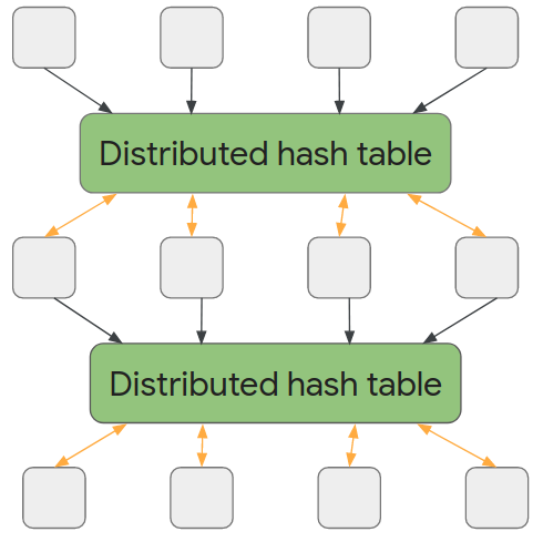
Tables in Napa are constantly updated, so we use log-structured merge forests (LSM tree) to organize the deluge of table updates. LSM is a forest of sorted data that is temporally organized with a B-tree index to support efficient key lookup queries. B-trees store summary information of the sub-trees in a hierarchical manner. Each B-tree node records the number of entries present in each subtree, which aids in the parallelization of queries. LSM allows us to decouple the process of updating the tables from the mechanics of query serving in the sense that live queries go against a different version of the data, which is atomically updated once the next batch of ingest (called delta) has been fully prepared for querying.


The partitioning problem

The data partitioning problem in our context is that we have a massively large table that is represented as an LSM tree. In the figure below, Delta 1 and 2 each have their own B-tree, and together represent 70 records. Napa breaks the records into two pieces, and assigns each piece to a different machine. The problem becomes a partitioning problem of a forest of trees and requires a tree-traversal algorithm that can quickly split the trees into two equal parts.

To avoid visiting all the nodes of the tree, we introduce the concept of “good enough” partitioning. As we begin cutting and partitioning the tree into two parts, we maintain an estimate of how bad our current answer would be if we terminated the partitioning process at that instant. This is the yardstick of how close we are to the answer and is represented below by a total error margin of 40 (at this point of execution, the two pieces are expected to be between 15 and 35 records in size, the uncertainty adds up to 40). Each subsequent traversal step reduces the error estimate, and if the two pieces are approximately equal, it stops the partitioning process. This process continues until the desired error margin is reached, at which time we are guaranteed that the two pieces are more or less equal.


Progressive partitioning algorithm

Progressive partitioning encapsulates the notion of “good enough” in that it makes a series of moves to reduce the error estimate. The input is a set of B-trees and the goal is to cut the trees into pieces of more or less equal size. The algorithm traverses one of the trees (“drill down'' in the figure) which results in a reduction of the error estimate. The algorithm is guided by statistics that are stored with each node of the tree so that it makes an informed set of moves at each step. The challenge here is to decide how to direct effort in the best possible way so that the error bound reduces quickly in the fewest possible steps. Progressive partitioning is conducive for our use-case since the longer the algorithm runs, the more equal the pieces become. It also means that if the algorithm is stopped at any point, one still gets good partitioning, where the quality corresponds to the time spent.

Prior work in this space uses a sampled table to drive the partitioning process, while the Napa approach uses a B-tree. As mentioned earlier, even just a sample from a petabyte table can be massive. A tree-based partitioning method can achieve partitioning much more efficiently than a sample-based approach, which does not use a tree organization of the sampled records. We compare progressive partitioning with an alternative approach, where sampling of the table at various resolutions (e.g., 1 record sample every 250 MB and so on) aids the partitioning of the query. Experimental results show the relative speedup from progressive partitioning for queries requiring varying numbers of machines. These results demonstrate that progressive partitioning is much faster than existing approaches and the speedup increases as the size of the query increases.


Conclusion

Napa's progressive partitioning algorithm efficiently optimizes database queries, enabling Google Ads to serve client reporting queries billions of times each day. We note that tree traversal is a common technique that students in introductory computer science courses use, yet it also serves a critical use-case at Google. We hope that this article will inspire our readers, as it demonstrates how simple techniques and carefully designed data structures can be remarkably potent if used well. Check out the paper and a recent talk describing Napa to learn more.


Acknowledgements

This blog post describes a collaborative effort between Junichi Tatemura, Tao Zou, Jagan Sankaranarayanan, Yanlai Huang, Jim Chen, Yupu Zhang, Kevin Lai, Hao Zhang, Gokul Nath Babu Manoharan, Goetz Graefe, Divyakant Agrawal, Brad Adelberg, Shilpa Kolhar and Indrajit Roy.

Source: Google AI Blog


Open Source Vizier: Towards reliable and flexible hyperparameter and blackbox optimization

Google Vizier is the de-facto system for blackbox optimization over objective functions and hyperparameters across Google, having serviced some of Google’s largest research efforts and optimized a wide range of products (e.g., Search, Ads, YouTube). For research, it has not only reduced language model latency for users, designed computer architectures, accelerated hardware, assisted protein discovery, and enhanced robotics, but also provided a reliable backend interface for users to search for neural architectures and evolve reinforcement learning algorithms. To operate at the scale of optimizing thousands of users’ critical systems and tuning millions of machine learning models, Google Vizier solved key design challenges in supporting diverse use cases and workflows, while remaining strongly fault-tolerant.

Today we are excited to announce Open Source (OSS) Vizier (with an accompanying systems whitepaper published at AutoML Conference 2022), a standalone Python package based on Google Vizier. OSS Vizier is designed for two main purposes: (1) managing and optimizing experiments at scale in a reliable and distributed manner for users, and (2) developing and benchmarking algorithms for automated machine learning (AutoML) researchers.


System design

OSS Vizier works by having a server provide services, namely the optimization of blackbox objectives, or functions, from multiple clients. In the main workflow, a client sends a remote procedure call (RPC) and asks for a suggestion (i.e., a proposed input for the client’s blackbox function), from which the service begins to spawn a worker to launch an algorithm (i.e., a Pythia policy) to compute the following suggestions. The suggestions are then evaluated by clients to form their corresponding objective values and measurements, which are sent back to the service. This pipeline is repeated multiple times to form an entire tuning trajectory.

The use of the ubiquitous gRPC library, which is compatible with most programming languages, such as C++ and Rust, allows maximum flexibility and customization, where the user can also write their own custom clients and even algorithms outside of the default Python interface. Since the entire process is saved to an SQL datastore, a smooth recovery is ensured after a crash, and usage patterns can be stored as valuable datasets for research into meta-learning and multitask transfer-learning methods such as the OptFormer and HyperBO.

In the distributed pipeline, multiple clients each send a “Suggest” request to the Service API, which produces Suggestions for the clients using Pythia. The clients evaluate these suggestions and return measurements. All transactions are stored to allow fault-tolerance.

Usage

Because of OSS Vizier’s emphasis as a service, in which clients can send requests to the server at any point in time, it is thus designed for a broad range of scenarios — the budget of evaluations, or trials, can range from tens to millions, and the evaluation latency can range from seconds to weeks. Evaluations can be done asynchronously (e.g., tuning an ML model) or in synchronous batches (e.g., wet lab settings involving multiple simultaneous experiments). Furthermore, evaluations may fail due to transient errors and be retried, or may fail due to persistent errors (e.g., the evaluation is impossible) and should not be retried.

This broadly supports a variety of applications, which include hyperparameter tuning deep learning models or optimizing non-computational objectives, which can be e.g., physical, chemical, biological, mechanical, or even human-evaluated, such as cookie recipes.

The OSS Vizier API allows (1) developers to integrate other packages, with PyGlove and Vertex Vizier already included, and (2) users to optimize their experiments, such as machine learning pipelines and cookie recipes.

Integrations, algorithms, and benchmarks

As Google Vizier is heavily integrated with many of Google’s internal frameworks and products, OSS Vizier will naturally be heavily integrated with many of Google’s open source and external frameworks. Most prominently, OSS Vizier will serve as a distributed backend for PyGlove to allow large-scale evolutionary searches over combinatorial primitives such as neural architectures and reinforcement learning algorithms. Furthermore, OSS Vizier shares the same client-based API with Vertex Vizier, allowing users to quickly swap between open-source and production-quality services.

For AutoML researchers, OSS Vizier is also outfitted with a useful collection of algorithms and benchmarks (i.e., objective functions) unified under common APIs for assessing the strengths and weaknesses of proposed methods. Most notably, via TensorFlow Probability, researchers can now use the JAX-based Gaussian Process Bandit algorithm, based on the default algorithm in Google Vizier that tunes internal users’ objectives.


Resources and future direction

We provide links to the codebase, documentation, and systems whitepaper. We plan to allow user contributions, especially in the form of algorithms and benchmarks, and further integrate with the open-source AutoML ecosystem. Going forward, we hope to see OSS Vizier as a core tool for expanding research and development over blackbox optimization and hyperparameter tuning.


Acknowledgements

OSS Vizier was developed by members of the Google Vizier team in collaboration with the TensorFlow Probability team: Setareh Ariafar, Lior Belenki, Emily Fertig, Daniel Golovin, Tzu-Kuo Huang, Greg Kochanski, Chansoo Lee, Sagi Perel, Adrian Reyes, Xingyou (Richard) Song, and Richard Zhang.

In addition, we thank Srinivas Vasudevan, Jacob Burnim, Brian Patton, Ben Lee, Christopher Suter, and Rif A. Saurous for further TensorFlow Probability integrations, Daiyi Peng and Yifeng Lu for PyGlove integrations, Hao Li for Vertex/Cloud integrations, Yingjie Miao for AutoRL integrations, Tom Hennigan, Varun Godbole, Pavel Sountsov, Alexey Volkov, Mihir Paradkar, Richard Belleville, Bu Su Kim, Vytenis Sakenas, Yujin Tang, Yingtao Tian, and Yutian Chen for open source and infrastructure help, and George Dahl, Aleksandra Faust, Claire Cui, and Zoubin Ghahramani for discussions.

Finally we thank Tom Small for designing the animation for this post.

Source: Google AI Blog


Alpa: Automated Model-Parallel Deep Learning

Over the last several years, the rapidly growing size of deep learning models has quickly exceeded the memory capacity of single accelerators. Earlier models like BERT (with a parameter size of < 1GB) can efficiently scale across accelerators by leveraging data parallelism in which model weights are duplicated across accelerators while only partitioning and distributing the training data. However, recent large models like GPT-3 (with a parameter size of 175GB) can only scale using model parallel training, where a single model is partitioned across different devices.

While model parallelism strategies make it possible to train large models, they are more complex in that they need to be specifically designed for target neural networks and compute clusters. For example, Megatron-LM uses a model parallelism strategy to split the weight matrices by rows or columns and then synchronizes results among devices. Device placement or pipeline parallelism partitions different operators in a neural network into multiple groups and the input data into micro-batches that are executed in a pipelined fashion. Model parallelism often requires significant effort from system experts to identify an optimal parallelism plan for a specific model. But doing so is too onerous for most machine learning (ML) researchers whose primary focus is to run a model and for whom the model’s performance becomes a secondary priority. As such, there remains an opportunity to automate model parallelism so that it can easily be applied to large models.

In “Alpa: Automating Inter- and Intra-Operator Parallelism for Distributed Deep Learning”, published at OSDI 2022, we describe a method for automating the complex model parallelism process. We demonstrate that with only one line of code Alpa can transform any JAX neural network into a distributed version with an optimal parallelization strategy that can be executed on a user-provided device cluster. We are also excited to release Alpa’s code to the broader research community.

Alpa Design
We begin by grouping existing ML parallelization strategies into two categories, inter-operator parallelism and intra-operator parallelism. Inter-operator parallelism assigns distinct operators to different devices (e.g., device placement) that are often accelerated with a pipeline execution schedule (e.g., pipeline parallelism). With intra-operator parallelism, which includes data parallelism (e.g., Deepspeed-Zero), operator parallelism (e.g., Megatron-LM), and expert parallelism (e.g., GShard-MoE), individual operators are split and executed on multiple devices, and often collective communication is used to synchronize the results across devices.

The difference between these two approaches maps naturally to the heterogeneity of a typical compute cluster. Inter-operator parallelism has lower communication bandwidth requirements because it is only transmitting activations between operators on different accelerators. But, it suffers from device underutilization because of its pipeline data dependency, i.e., some operators are inactive while waiting on the outputs from other operators. In contrast, intra-operator parallelism doesn’t have the data dependency issue, but requires heavier communication across devices. In a GPU cluster, the GPUs within a node have higher communication bandwidth that can accommodate intra-operator parallelism. However, GPUs across different nodes are often connected with much lower bandwidth (e.g., ethernet) so inter-operator parallelism is preferred.

By leveraging heterogeneous mapping, we design Alpa as a compiler that conducts various passes when given a computational graph and a device cluster from a user. First, the inter-operator pass slices the computational graph into subgraphs and the device cluster into submeshes (i.e., a partitioned device cluster) and identifies the best way to assign a subgraph to a submesh. Then, the intra-operator pass finds the best intra-operator parallelism plan for each pipeline stage from the inter-operator pass. Finally, the runtime orchestration pass generates a static plan that orders the computation and communication and executes the distributed computational graph on the actual device cluster.

An overview of Alpa. In the sliced subgraphs, red and blue represent the way the operators are partitioned and gray represents operators that are replicated. Green represents the actual devices (e.g., GPUs).

Intra-Operator Pass
Similar to previous research (e.g., Mesh-TensorFlow and GSPMD), intra-operator parallelism partitions a tensor on a device mesh. This is shown below for a typical 3D tensor in a Transformer model with a given batch, sequence, and hidden dimensions. The batch dimension is partitioned along device mesh dimension 0 (mesh0), the hidden dimension is partitioned along mesh dimension 1 (mesh1), and the sequence dimension is replicated to each processor.

A 3D tensor that is partitioned on a 2D device mesh.

With the partitions of tensors in Alpa, we further define a set of parallelization strategies for each individual operator in a computational graph. We show example parallelization strategies for matrix multiplication in the figure below. Defining parallelization strategies on operators leads to possible conflicts on the partitions of tensors because one tensor can be both the output of one operator and the input of another. In this case, re-partition is needed between the two operators, which incurs additional communication costs.

The parallelization strategies for matrix multiplication.

Given the partitions of each operator and re-partition costs, we formulate the intra-operator pass as a Integer-Linear Programming (ILP) problem. For each operator, we define a one-hot variable vector to enumerate the partition strategies. The ILP objective is to minimize the sum of compute and communication cost (node cost) and re-partition communication cost (edge cost). The solution of the ILP translates to one specific way to partition the original computational graph.

Inter-Operator Pass
The inter-operator pass slices the computational graph and device cluster for pipeline parallelism. As shown below, the boxes represent micro-batches of input and the pipeline stages represent a submesh executing a subgraph. The horizontal dimension represents time and shows the pipeline stage at which a micro-batch is executed. The goal of the inter-operator pass is to minimize the total execution latency, which is the sum of the entire workload execution on the device as illustrated in the figure below. Alpa uses a Dynamic Programming (DP) algorithm to minimize the total latency. The computational graph is first flattened, and then fed to the intra-operator pass where the performance of all possible partitions of the device cluster into submeshes are profiled.

Pipeline parallelism. For a given time, this figure shows the micro-batches (colored boxes) that a partitioned device cluster and a sliced computational graph (e.g., stage 1, 2, 3) is processing.

Runtime Orchestration
After the inter- and intra-operator parallelization strategies are complete, the runtime generates and dispatches a static sequence of execution instructions for each device submesh. These instructions include RUN a specific subgraph, SEND/RECEIVE tensors from other meshes, or DELETE a specific tensor to free the memory. The devices can execute the computational graph without other coordination by following the instructions.

Evaluation
We test Alpa with eight AWS p3.16xlarge instances, each of which has eight 16 GB V100 GPUs, for 64 total GPUs. We examine weak scaling results of growing the model size while increasing the number of GPUs. We evaluate three models: (1) the standard Transformer model (GPT); (2) the GShard-MoE model, a transformer with mixture-of-expert layers; and (3) Wide-ResNet, a significantly different model with no existing expert-designed model parallelization strategy. The performance is measured by peta-floating point operations per second (PFLOPS) achieved on the cluster.

We demonstrate that for GPT, Alpa outputs a parallelization strategy very similar to the one computed by the best existing framework, Megatron-ML, and matches its performance. For GShard-MoE, Alpa outperforms the best expert-designed baseline on GPU (i.e., Deepspeed) by up to 8x. Results for Wide-ResNet show that Alpa can generate the optimal parallelization strategy for models that have not been studied by experts. We also show the linear scaling numbers for reference.

GPT: Alpa matches the performance of Megatron-ML, the best expert-designed framework.
GShard MoE: Alpa outperforms Deepspeed (the best expert-designed framework on GPU) by up to 8x.
Wide-ResNet: Alpa generalizes to models without manual plans. Pipeline and Data Parallelism (PP-DP) is a baseline model that uses only pipeline and data parallelism but no other intra-operator parallelism.
The parallelization strategy for Wide-ResNet on 16 GPUs consists of three pipeline stages and is a complicated strategy even for an expert to design. Stages 1 and 2 are on 4 GPUs performing data parallelism, and stage 3 is on 8 GPUs performing operator parallelism.

Conclusion
The process of designing an effective parallelization plan for distributed model-parallel deep learning has historically been a difficult and labor-intensive task. Alpa is a new framework that leverages intra- and inter-operator parallelism for automated model-parallel distributed training. We believe that Alpa will democratize distributed model-parallel learning and accelerate the development of large deep learning models. Explore the open-source code and learn more about Alpa in our paper.

Acknowledgements
Thanks to the co-authors of the paper: Lianmin Zheng, Hao Zhang, Yonghao Zhuang, Yida Wang, Danyang Zhuo, Joseph E. Gonzalez, and Ion Stoica. We would also like to thank Shibo Wang, Jinliang Wei, Yanping Huang, Yuanzhong Xu, Zhifeng Chen, Claire Cui, Naveen Kumar, Yash Katariya, Laurent El Shafey, Qiao Zhang, Yonghui Wu, Marcello Maggioni, Mingyao Yang, Michael Isard, Skye Wanderman-Milne, and David Majnemer for their collaborations to this research.


Source: Google AI Blog


Large-Scale Matrix Factorization on TPUs

Matrix factorization is one of the oldest, yet still widely used, techniques for learning how to recommend items such as songs or movies from user ratings. In its basic form, it approximates a large, sparse (i.e., mostly empty) matrix of user-item interactions with a product of two smaller, denser matrices representing learned item and user features. These dense matrices, in turn, can be used to recommend items to a user with which they haven't interacted before.

Despite its algorithmic simplicity, matrix factorization can still achieve competitive performance in recommender benchmarks. Alternating least squares (ALS), and especially its implicit variation, is a fundamental algorithm to learn the parameters of matrix factorization. ALS is known for its high efficiency because it scales linearly in the number of rows, columns and non-zeros. Hence, this algorithm is very well suited for large-scale challenges. But, for very large real-world matrix factorization datasets, a single machine implementation would not suffice, and so, it would require a large distributed system. Most of the distributed implementations of matrix factorization that employ ALS leverage off-the-shelf CPU devices, and rightfully so, due to the inherently sparse nature of the problem (the input matrix is mostly empty).

On the other hand, recent success of deep learning, which has exhibited growing computational capacity, has spurred a new wave of research and progress on hardware accelerators such as Tensor Processing Units (TPUs). TPUs afford domain specific hardware speedups, especially for use cases like deep learning, which involves a large number of dense matrix multiplications. In particular, they allow significant speedups for traditional data-parallel workloads, such as training models with Stochastic Gradient Descent (SGD) in SPMD (single program multiple data) fashion. The SPMD approach has gained popularity in computations like training neural networks with gradient descent algorithms, and can be used for both data-parallel and model-parallel computations, where we distribute parameters of the model across available devices. Nevertheless, while TPUs have been enormously attractive for methods based on SGD, it is not immediately clear if a high performance implementation of ALS, which requires a large number of distributed sparse matrix multiplies, can be developed for a large-scale cluster of TPU devices.

In “ALX: Large Scale Matrix Factorization on TPUs”, we explore a distributed ALS design that makes efficient use of the TPU architecture and can scale well to matrix factorization problems of the order of billions of rows and columns by scaling the number of available TPU cores. The approach we propose leverages a combination of model and data parallelism, where each TPU core both stores a portion of the embedding table and trains over a unique slice of data, grouped in mini-batches. In order to spur future research on large-scale matrix factorization methods and to illustrate the scalability properties of our own implementation, we also built and released a real world web link prediction dataset called WebGraph.

The figure shows the flow of data and computation through the ALX framework on TPU devices. Similar to SGD-based training procedures, each TPU core performs identical computation for its own batch of data in SPMD fashion, which allows for synchronous computation in parallel on multiple TPU cores. Each TPU starts with gathering all the relevant item embeddings in the Sharded Gather stage. These materialized embeddings are used to solve for user embeddings which are scattered to the relevant shard of the embedding table in the Sharded Scatter stage.

Dense Batching for Improved Efficiency
We designed ALX specifically for TPUs, exploiting unique properties of TPU architecture while overcoming a few interesting limitations. For instance, each TPU core has limited memory and restricts all tensors to have a static shape, but each example in a mini-batch can have a wildly varying number of items (i.e., inputs can be long and sparse). To resolve this, we break exceedingly long examples into multiple smaller examples of the same shape, a process called dense batching. More details about dense batching can be found in our paper.

Illustrating example of how sparse batches are densified to increase efficiency on TPUs.

Uniform Sharding of Embedding Tables
With the batching problem solved, we next want to factorize a sparse matrix into two dense embedding matrices (e.g., user and item embeddings) such that the resulting dot product of embeddings approximate the original sparse matrix — this helps us infer predictions for all the positions from the original matrix, including those that were empty, which can be used to recommend items with which users haven’t interacted. Both the resulting embedding tables (W and H in the figure below) can potentially be too large to fit in a single TPU core, thus requiring a distributed training setup for most large-scale use cases.

Most previous attempts of distributed matrix factorization use a parameter server architecture where the model parameters are stored on highly available servers, and the training data is processed in parallel by workers that are solely responsible for the learning task. In our case, since each TPU core has identical compute and memory, it's wasteful to only use either memory for storing model parameters or compute for training. Thus, we designed our system such that each core is used to do both.

Illustrative example of factorizing a sparse matrix Y into two dense embedding matrices W and H.

In ALX, we uniformly divide both embedding tables, thus fully exploiting both the size of distributed memory available and the dedicated low-latency interconnects between TPUs. This is highly efficient for very large embedding tables and results in good performance for distributed gather and scatter operations.

Uniform sharding of both embedding tables (W and H) across TPU cores (in blue).

WebGraph
Since potential applications may involve very large data sets, scalability is potentially an important opportunity for advancement in matrix factorization. To that end, we also release a large real-world web link prediction dataset called WebGraph. This dataset can be easily modeled as a matrix factorization problem where rows and columns are source and destination links, respectively, and the task is to predict destination links from each source link. We use WebGraph to illustrate the scaling properties of ALX.

The WebGraph dataset was generated from a single crawl performed by CommonCrawl in 2021 where we strip everything and keep only the link->outlinks data. Since the performance of a factorization method depends on the properties of the underlying graph, we created six versions of WebGraph, each varying in the sparsity pattern and locale, to study how well ALS performs on each.

  • To study locale-specific graphs, we filter based on two top level domains: ‘de’ and ‘in’, each producing a graph with an order of magnitude fewer nodes.
  • These graphs can still have arbitrary sparsity patterns and dangling links. Thus we further filter the nodes in each graph to have a minimum of either 10 or 50 inlinks and outlinks.

For easy access, we have made these available as a Tensorflow Dataset package. For reference, the biggest version, WebGraph-sparse, has more than 365M nodes and 30B edges. We create and publish both training and testing splits for evaluation purposes.

Results
We carefully tune the system and quality parameters of ALX. Based on our observations related to precision and choice of linear solvers. ​​We observed that by carefully selecting the precision for storage of the embedding tables (bfloat16) and for the input to the linear solvers (float32), we were able to halve the memory required for the embeddings while still avoiding problems arising from lower precision values during the solve stage. For our linear solvers, we selected conjugate gradients, which we found to be the fastest across the board on TPUs. We use embeddings of dimension 128 and train the model for 16 epochs. In our experience, hyperparameter tuning over both norm penalty (λ) and unobserved weight (α) has been indispensable for good recall metrics as shown in the table below.

Results obtained by running ALX on all versions of WebGraph dataset. Recall values of 1.0 denote perfect recall.

Scaling Analysis
Since the input data are processed in parallel across TPU cores, increasing the number of cores decreases training time, ideally in a linear fashion. But at the same time, a larger number of cores requires more network communication (due to the sharded embedding tables). Thanks to high-speed interconnects, this overhead can be negligible for a small number of cores, but as the number of cores increases, the overhead eventually slows down the ideal linear scaling.

In order to confirm our hypothesis, we analyze scaling properties of the four biggest WebGraph variants in terms of training time as we increase the number of available TPU cores. As shown below, even empirically, we do observe the predicted linear decrease in training time up to a sweet spot, after which the network overhead slows the decline.

Scaling analysis of running time as the number of TPU cores are increased. Each figure plots the time taken to train for one epoch in seconds.

Conclusion
For easy access and reproducibility, the ALX code is open-sourced and can be easily run on Google Cloud. In fact, we illustrate that a sparse matrix like WebGraph-dense of size 135M x 135M (with 22B edges) can be factorized in a colab connected to 8 TPU cores in less than a day. We have designed the ALX framework with scalability in mind. With 256 TPU cores, one epoch of the largest WebGraph variant, WebGraph-sparse (365M x 365M sparse matrix) takes around 20 minutes to finish (5.5 hours for the whole training run). The final model has around 100B parameters. We hope that the ALX and WebGraph will be useful to both researchers and practitioners working in these fields. The code for ALX can be found here on github!

Acknowledgements
The core team includes Steffen Rendle, Walid Krichene and Li Zhang. We thank many Google colleagues for helping at various stages of this project. In particular, we are grateful to the JAX team for numerous discussions, especially James Bradbury and Skye Wanderman-Milne; Blake Hechtman for help with XLA and Rasmus Larsen for useful discussions about performance of linear solvers on TPUs. Finally, we're also grateful to Nicolas Mayoraz, John Anderson, and Fernando Pereira for providing useful feedback.

Source: Google AI Blog


A Scalable Approach for Partially Local Federated Learning

Federated learning enables users to train a model without sending raw data to a central server, thus avoiding the collection of privacy-sensitive data. Often this is done by learning a single global model for all users, even though the users may differ in their data distributions. For example, users of a mobile keyboard application may collaborate to train a suggestion model but have different preferences for the suggestions. This heterogeneity has motivated algorithms that can personalize a global model for each user.

However, in some settings privacy considerations may prohibit learning a fully global model. Consider models with user-specific embeddings, such as matrix factorization models for recommender systems. Training a fully global federated model would involve sending user embedding updates to a central server, which could potentially reveal the preferences encoded in the embeddings. Even for models without user-specific embeddings, having some parameters be completely local to user devices would reduce server-client communication and responsibly personalize those parameters to each user.

Left: A matrix factorization model with a user matrix P and items matrix Q. The user embedding for a user u (Pu) and item embedding for item i (Qi) are trained to predict the user’s rating for that item (Rui). Right: Applying federated learning approaches to learn a global model can involve sending updates for Pu to a central server, potentially leaking individual user preferences.

In “Federated Reconstruction: Partially Local Federated Learning”, presented at NeurIPS 2021, we introduce an approach that enables scalable partially local federated learning, where some model parameters are never aggregated on the server. For matrix factorization, this approach trains a recommender model while keeping user embeddings local to each user device. For other models, this approach trains a portion of the model to be completely personal for each user while avoiding communication of these parameters. We successfully deployed partially local federated learning to Gboard, resulting in better recommendations for hundreds of millions of keyboard users. We’re also releasing a TensorFlow Federated tutorial demonstrating how to use Federated Reconstruction.

Federated Reconstruction
Previous approaches for partially local federated learning used stateful algorithms, which require user devices to store a state across rounds of federated training. Specifically, these approaches required devices to store local parameters across rounds. However, these algorithms tend to degrade in large-scale federated learning settings. In these cases, the majority of users do not participate in training, and users who do participate likely only do so once, resulting in a state that is rarely available and can get stale across rounds. Also, all users who do not participate are left without trained local parameters, preventing practical applications.

Federated Reconstruction is stateless and avoids the need for user devices to store local parameters by reconstructing them whenever needed. When a user participates in training, before updating any globally aggregated model parameters, they randomly initialize and train their local parameters using gradient descent on local data with global parameters frozen. They can then calculate updates to global parameters with local parameters frozen. A round of Federated Reconstruction training is depicted below.

Models are partitioned into global and local parameters. For each round of Federated Reconstruction training: (1) The server sends the current global parameters g to each user i; (2) Each user i freezes g and reconstructs their local parameters li; (3) Each user i freezes li and updates g to produce gi; (4) Users’ gi are averaged to produce the global parameters for the next round. Steps (2) and (3) generally use distinct parts of the local data.

This simple approach avoids the challenges of previous methods. It does not assume users have a state from previous rounds of training, enabling large-scale training, and local parameters are always freshly reconstructed, preventing staleness. Users unseen during training can still get trained models and perform inference by simply reconstructing local parameters using local data.

Federated Reconstruction trains better performing models for unseen users compared to other approaches. For a matrix factorization task with unseen users, the approach significantly outperforms both centralized training and baseline Federated Averaging.

RMSE ↓ Accuracy ↑
Centralized 1.36 40.8%
FedAvg .934 40.0%
FedRecon (this work) .907 43.3%
Root-mean-square-error (lower is better) and accuracy for a matrix factorization task with unseen users. Centralized training and Federated Averaging (FedAvg) both reveal privacy-sensitive user embeddings to a central server, while Federated Reconstruction (FedRecon) avoids this.

These results can be explained via a connection to meta learning (i.e., learning to learn); Federated Reconstruction trains global parameters that lead to fast and accurate reconstruction of local parameters for unseen users. That is, Federated Reconstruction is learning to learn local parameters. In practice, we observe that just one gradient descent step can yield successful reconstruction, even for models with about one million local parameters.

Federated Reconstruction also provides a way to personalize models for heterogeneous users while reducing communication of model parameters — even for models without user-specific embeddings. To evaluate this, we apply Federated Reconstruction to personalize a next word prediction language model and observe a substantial increase in performance, attaining accuracy on par with other personalization methods despite reduced communication. Federated Reconstruction also outperforms other personalization methods when executed at a fixed communication level.

Accuracy ↑ Communication ↓
FedYogi 24.3% Whole Model
FedYogi + Finetuning 30.8% Whole Model
FedRecon (this work) 30.7% Partial Model
Accuracy and server-client communication for a next word prediction task without user-specific embeddings. FedYogi communicates all model parameters, while FedRecon avoids this.

Real-World Deployment in Gboard
To validate the practicality of Federated Reconstruction in large-scale settings, we deployed the algorithm to Gboard, a mobile keyboard application with hundreds of millions of users. Gboard users use expressions (e.g., GIFs, stickers) to communicate with others. Users have highly heterogeneous preferences for these expressions, making the setting a good fit for using matrix factorization to predict new expressions a user might want to share.

Gboard users can communicate with expressions, preferences for which are highly personal.

We trained a matrix factorization model over user-expression co-occurrences using Federated Reconstruction, keeping user embeddings local to each Gboard user. We then deployed the model to Gboard users, leading to a 29.3% increase in click-through-rate for expression recommendations. Since most Gboard users were unseen during federated training, Federated Reconstruction played a key role in this deployment.

Further Explorations
We’ve presented Federated Reconstruction, a method for partially local federated learning. Federated Reconstruction enables personalization to heterogeneous users while reducing communication of privacy-sensitive parameters. We scaled the approach to Gboard in alignment with our AI Principles, improving recommendations for hundreds of millions of users.

For a technical walkthrough of Federated Reconstruction for matrix factorization, check out the TensorFlow Federated tutorial. We’ve also released general-purpose TensorFlow Federated libraries and open-source code for running experiments.

Acknowledgements
Karan Singhal, Hakim Sidahmed, Zachary Garrett, Shanshan Wu, Keith Rush, and Sushant Prakash co-authored the paper. Thanks to Wei Li, Matt Newton, and Yang Lu for their partnership on Gboard deployment. We’d also like to thank Brendan McMahan, Lin Ning, Zachary Charles, Warren Morningstar, Daniel Ramage, Jakub Konecný, Alex Ingerman, Blaise Agüera y Arcas, Jay Yagnik, Bradley Green, and Ewa Dominowska for their helpful comments and support.

Source: Google AI Blog


General and Scalable Parallelization for Neural Networks

Scaling neural networks, whether it be the amount of training data used, the model size or the computation being utilized, has been critical for improving model quality in many real-world machine learning applications, such as computer vision, language understanding and neural machine translation. This, in turn, has motivated recent studies to scrutinize the factors that play a critical role in the success of scaling a neural model. Although increasing model capacity can be a sound approach to improve model quality, doing so presents a number of systems and software engineering challenges that must be overcome. For instance, in order to train large models that exceed the memory capacity of an accelerator, it becomes necessary to partition the weights and the computation of the model across multiple accelerators. This process of parallelization increases the network communication overhead and can result in device under-utilization. Moreover, a given algorithm for parallelization, which typically requires a significant amount of engineering effort, may not work with different model architectures.

To address these scaling challenges, we present “GSPMD: General and Scalable Parallelization for ML Computation Graphs”, in which we describe an open-source automatic parallelization system based on the XLA compiler. GSPMD is capable of scaling most deep learning network architectures and has already been applied to many deep learning models, such as GShard-M4, LaMDA, BigSSL, ViT, and MetNet-2, leading to state-of-the-art-results across several domains. GSPMD has also been integrated into multiple ML frameworks, including TensorFlow and JAX, which use XLA as a shared compiler.

Overview
GSPMD separates the task of programming an ML model from the challenge of parallelization. It allows model developers to write programs as if they were run on a single device with very high memory and computation capacity — the user simply needs to add a few lines of annotation code to a subset of critical tensors in the model code to indicate how to partition the tensors. For example, to train a large model-parallel Transformer, one may only need to annotate fewer than 10 tensors (less than 1% of all tensors in the entire computation graph), one line of additional code per tensor. Then GSPMD runs a compiler pass that determines the entire graph's parallelization plan, and transforms it into a mathematically equivalent, parallelized computation that can be executed on each device. This allows users to focus on model building instead of parallelization implementation, and enables easy porting of existing single-device programs to run at a much larger scale.

The separation of model programming and parallelism also allows developers to minimize code duplication. With GSPMD, developers may employ different parallelism algorithms for different use cases without the need to reimplement the model. For example, the model code that powered the GShard-M4 and LaMDA models can apply a variety of parallelization strategies appropriate for different models and cluster sizes with the same model implementation. Similarly, by applying GSPMD, the BigSSL large speech models can share the same implementation with previous smaller models.

Generality and Flexibility
Because different model architectures may be better suited to different parallelization strategies, GSPMD is designed to support a large variety of parallelism algorithms appropriate for different use cases. For example, with smaller models that fit within the memory of a single accelerator, data parallelism is preferred, in which devices train the same model using different input data. In contrast, models that are larger than a single accelerator’s memory capacity are better suited for a pipelining algorithm (like that employed by GPipe) that partitions the model into multiple, sequential stages, or operator-level parallelism (e.g., Mesh-TensorFlow), in which individual computation operators in the model are split into smaller, parallel operators.

GSPMD supports all the above parallelization algorithms with a uniform abstraction and implementation. Moreover, GSPMD supports nested patterns of parallelism. For example, it can be used to partition models into individual pipeline stages, each of which can be further partitioned using operator-level parallelism.

GSPMD also facilitates innovation on parallelism algorithms by allowing performance experts to focus on algorithms that best utilize the hardware, instead of the implementation that involves lots of cross-device communications. For example, for large Transformer models, we found a novel operator-level parallelism algorithm that partitions multiple dimensions of tensors on a 2D mesh of devices. It reduces peak accelerator memory usage linearly with the number of training devices, while maintaining a high utilization of accelerator compute due to its balanced data distribution over multiple dimensions.

To illustrate this, consider a simplified feedforward layer in a Transformer model that has been annotated in the above way. To execute the first matrix multiply on fully partitioned input data, GSPMD applies an MPI-style AllGather communication operator to partially merge with partitioned data from another device. It then executes the matrix multiply locally and produces a partitioned result. Before the second matrix multiply, GSPMD adds another AllGather on the right-hand side input, and executes the matrix multiply locally, yielding intermediate results that will then need to be combined and partitioned. For this, GSPMD adds an MPI-style ReduceScatter communication operator that accumulates and partitions these intermediate results. While the tensors generated with the AllGather operator at each stage are larger than the original partition size, they are short-lived and the corresponding memory buffers will be freed after use, which does not affect peak memory usage in training.

Left: A simplified feedforward layer of a Transformer model. Blue rectangles represent tensors with dashed red & blue lines overlaid representing the desired partitioning across a 2x2 mesh of devices. Right: A single partition, after GSPMD has been applied.

A Transformer Example with Nested Parallelism
As a shared, robust mechanism for different parallelism modes, GSPMD allows users to conveniently switch between modes in different parts of a model. This is particularly valuable for models that may have different components with distinct performance characteristics, for example, multimodal models that handle both images and audio. Consider a model with the Transformer encoder-decoder architecture, which has an embedding layer, an encoder stack with Mixture-of-Expert layers, a decoder stack with dense feedforward layers, and a final softmax layer. In GSPMD, a complex combination of several parallelism modes that treats each layer separately can be achieved with simple configurations.

In the figure below, we show a partitioning strategy over 16 devices organized as a logical 4x4 mesh. Blue represents partitioning along the first mesh dimension X, and yellow represents partitioning along the second mesh dimension Y. X and Y are repurposed for different model components to achieve different parallelism modes. For example, the X dimension is used for data parallelism in the embedding and softmax layers, but used for pipeline parallelism in the encoder and decoder. The Y dimension is also used in different ways to partition the vocabulary, batch or model expert dimensions.

Computation Efficiency
GSPMD provides industry-leading performance in large model training. Parallel models require extra communication to coordinate multiple devices to do the computation. So parallel model efficiency can be estimated by examining the fraction of time spent on communication overhead — the higher percentage utilization and the less time spent on communication, the better. In the recent MLPerf set of performance benchmarks, a BERT-like encoder-only model with ~500 billion parameters to which we applied GSPMD for parallelization over 2048 TPU-V4 chips yielded highly competitive results (see table below), utilizing up to 63% of the peak FLOPS that the TPU-V4s offer. We also provide efficiency benchmarks for some representative large models in the table below. These example model configs are open sourced in the Lingvo framework along with instructions to run them on Google Cloud. More benchmark results can be found in the experiment section of our paper.

Model Family Parameter Count % of model activated* No. of Experts** No. of Layers No. of TPU FLOPS utilization
Dense Decoder (LaMDA) 137B 100% 1 64 1024 TPUv3 56.5%
Dense Encoder (MLPerf-Bert) 480B 100% 1 64 2048 TPUv4 63%
Sparsely Activated Encoder-Decoder (GShard-M4) 577B 0.25% 2048 32 1024 TPUv3 46.8%
Sparsely Activated Decoder 1.2T 8% 64 64 1024 TPUv3 53.8%
*The fraction of the model activated during inference, which is a measure of model sparsity.
**Number of experts included in the Mixture of Experts layer. A value of 1 corresponds to a standard Transformer, without a Mixture of Experts layer.

Conclusion
The ongoing development and success of many useful machine learning applications, such as NLP, speech recognition, machine translation, and autonomous driving, depend on achieving the highest accuracy possible. As this often requires building larger and even more complex models, we are pleased to share the GSPMD paper and the corresponding open-source library to the broader research community, and we hope it is useful for efficient training of large-scale deep neural networks.

Acknowledgements
We wish to thank Claire Cui, Zhifeng Chen, Yonghui Wu, Naveen Kumar, Macduff Hughes, Zoubin Ghahramani and Jeff Dean for their support and invaluable input. Special thanks to our collaborators Dmitry Lepikhin, HyoukJoong Lee, Dehao Chen, Orhan Firat, Maxim Krikun, Blake Hechtman, Rahul Joshi, Andy Li, Tao Wang, Marcello Maggioni, David Majnemer, Noam Shazeer, Ankur Bapna, Sneha Kudugunta, Quoc Le, Mia Chen, Shibo Wang, Jinliang Wei, Ruoming Pang, Zongwei Zhou, David So, Yanqi Zhou, Ben Lee, Jonathan Shen, James Qin, Yu Zhang, Wei Han, Anmol Gulati, Laurent El Shafey, Andrew Dai, Kun Zhang, Nan Du, James Bradbury, Matthew Johnson, Anselm Levskaya, Skye Wanderman-Milne‎, and Qiao Zhang for helpful discussions and inspirations.

Source: Google AI Blog


Massively Parallel Graph Computation: From Theory to Practice

Graphs are useful theoretical representations of the connections between groups of entities, and have been used for a variety of purposes in data science, from ranking web pages by popularity and mapping out social networks, to assisting with navigation. In many cases, such applications require the processing of graphs containing hundreds of billions of edges, which is far too large to be processed on a single consumer-grade machine. A typical approach to scaling graph algorithms is to run in a distributed setting, i.e., to partition the data (and the algorithm) among multiple computers to perform the computation in parallel. While this approach allows one to process graphs with trillions of edges, it also introduces new challenges. Namely, because each computer only sees a small piece of the input graph at a time, one needs to handle inter-machine communication and design algorithms that can be split across multiple computers.

A framework for implementing distributed algorithms, MapReduce, was introduced in 2008. It transparently handled communication between machines while offering good fault-tolerance capabilities and inspired the development of a number of distributed computation frameworks, including Pregel, Apache Hadoop, and many others. Still, the challenge of developing algorithms for distributed computation on very large graphs remained, and designing efficient algorithms in this context even for basic problems, such as connected components, maximum matching or shortest paths, has been an active area of research. While recent work has demonstrated new algorithms for many problems, including our algorithms for connected components (both in theory and practice) and hierarchical clustering, there was still a need for methods that could solve a range of problems more quickly.

Today we present a pair of recent papers that address this problem by first constructing a theoretical model for distributed graph algorithms and then demonstrating how the model can be applied. The proposed model, Adaptive Massively Parallel Computation (AMPC), augments the theoretical capabilities of MapReduce, providing a pathway to solve many graph problems in fewer computation rounds. We also show how the AMPC model can be effectively implemented in practice. The suite of algorithms we describe, which includes algorithms for maximal independent set, maximum matching, connected components and minimum spanning tree, work up to 7x faster than current state-of-the-art approaches.

Limitations of MapReduce
In order to understand the limitations of MapReduce for developing graph algorithms, consider a simplified variant of the connected components problem. The input is a collection of rooted trees, and the goal is to compute, for each node, the root of its tree. Even this seemingly simple problem is not easy to solve in MapReduce. In fact, in the Massively Parallel Computation (MPC) model — the theoretical model behind MapReduce, Pregel, Apache Giraph and many other distributed computation frameworks — this problem is widely believed to require at least a number of rounds of computation proportional to log n, where n is the total number of nodes in the graph. While log n may not seem to be a large number, algorithms processing trillion-edge graphs often write hundreds of terabytes of data to disk in each round, and thus even a small reduction in the number of rounds may bring significant resource savings.

The problem of finding root nodes. Nodes are represented by blue circles. Gray arrows point from each node to its parent. The root nodes are the nodes with no parents. The orange arrows illustrate the path an algorithm would follow from a node to the root of the tree to which it belongs.

A similar subproblem showed up in our algorithms for finding connected components and computing a hierarchical clustering. We observed that one can bypass the limitations of MapReduce by implementing these algorithms through the use of a distributed hash table (DHT), a service that is initialized with a collection of key-value pairs and then returns a value associated with a provided key in real-time. In our implementation, for each node, the DHT stores its parent node. Then, a machine that processes a graph node can use the DHT and “walk up” the tree until it reaches the root. While the use of a DHT worked well for this particular problem (although it relied on the input trees being not too deep), it was unclear if the idea could be applied more broadly.

The Adaptive Massively Parallel Computation Model
To extend this approach to other problems, we started by developing a model to theoretically analyze algorithms that utilize a DHT. The resulting AMPC model builds upon the well-established MPC model and formally describes the capabilities brought by the use of a distributed hash table.

In the MPC model there is a collection of machines, which communicate via message passing in synchronous rounds. Messages sent in one round are delivered in the beginning of the following round and constitute that round’s entire input (i.e., the machines do not retain information from one round to the next). In the first round, one can assume that the input is randomly distributed across the machines. The goal is to minimize the number of computation rounds, while assuring load-balancing between machines in each round.

Computation in the MPC model. Each column represents one machine in subsequent computation rounds. Once all machines have completed a round of computation, all messages sent in that round are delivered, and the following round begins.

We then formalized the AMPC model by introducing a new approach, in which machines write to a write-only distributed hash table each round, instead of communicating via messages. Once a new round starts, the hash table from the previous round becomes read-only and a new write-only output hash table becomes available. What is important is that only the method of communication changes — the amount of communication and available space per machine is constrained exactly in the same way as in the MPC model. Hence, at a high level the added capability of the AMPC model is that each machine can choose what data to read, instead of being provided a piece of data.

Computation in the AMPC model. Once all machines have completed a round of computation, the data they produced is saved to a distributed hash table. In the following round, each machine can read arbitrary values from this distributed hash table and write to a new distributed hash table.

Algorithms and Empirical Evaluation
This seemingly small difference in the way machines communicate allowed us to design much faster algorithms to a number of basic graph problems. In particular, we show that it is possible to find connected components, minimum spanning tree, maximal matching and maximal independent set in a constant number of rounds, regardless of the size of the graph.

To investigate the practical applicability of the AMPC algorithms, we have instantiated the model by combining Flume C++ (a C++ counterpart of FlumeJava) with a DHT communication layer. We have evaluated our AMPC algorithms for minimum spanning tree, maximal independent set and maximum matching and observed that we can achieve up to 7x speedups over implementations that did not use a DHT. At the same time, the AMPC implementations used 10x fewer rounds on average to complete, and also wrote less data to disk.

Our implementation of the AMPC model took advantage of hardware-accelerated remote direct memory access (RDMA), a technology that allows reading from the memory of a remote machine with a latency of a few microseconds, which is just an order of magnitude slower than reading from local memory. While some of the AMPC algorithms communicated more data than their MPC counterparts, they were overall faster, as they performed mostly fast reads using RDMA, instead of costly writes to disk.

Conclusion
With the AMPC model, we built a theoretical framework inspired by practically efficient implementations, and then developed new theoretical algorithms that delivered good empirical performance and maintained good fault-tolerance properties. We've been happy to see that the AMPC model has already been the subject of further study and are excited to learn what other problems can be solved more efficiently using the AMPC model or its practical implementations.

Acknowledgements
Co-authors on the two papers covered in this blog post include Soheil Behnezhad, Laxman Dhulipala, Hossein Esfandiari, and Warren Schudy. We also thank members of the Graph Mining team for their collaborations, and especially Mohammad Hossein Bateni for his input on this post. To learn more about our recent work on scalable graph algorithms, see videos from our recent Graph Mining and Learning workshop.

Source: Google AI Blog


Massively Large-Scale Distributed Reinforcement Learning with Menger

In the last decade, reinforcement learning (RL) has become one of the most promising research areas in machine learning and has demonstrated great potential for solving sophisticated real-world problems, such as chip placement and resource management, and solving challenging games (e.g., Go, Dota 2, and hide-and-seek). In simplest terms, an RL infrastructure is a loop of data collection and training, where actors explore the environment and collect samples, which are then sent to the learners to train and update the model. Most current RL techniques require many iterations over batches of millions of samples from the environment to learn a target task (e.g., Dota 2 learns from batches of 2 million frames every 2 seconds). As such, an RL infrastructure should not only scale efficiently (e.g., increase the number of actors) and collect an immense number of samples, but also be able to swiftly iterate over these extensive amounts of samples during training.

Overview of an RL system in which an actor sends trajectories (e.g., multiple samples) to a learner. The learner trains a model using the sampled data and pushes the updated model back to the actor (e.g. TF-Agents, IMPALA).

Today we introduce Menger1, a massive large-scale distributed RL infrastructure with localized inference that scales up to several thousand actors across multiple processing clusters (e.g., Borg cells), reducing the overall training time in the task of chip placement. In this post we describe how we implement Menger using Google TPU accelerators for fast training iterations, and present its performance and scalability on the challenging task of chip placement. Menger reduces the training time by up to 8.6x compared to a baseline implementation.

Menger System Design
There are various distributed RL systems, such as Acme and SEED RL, each of which focus on optimizing a single particular design point in the space of distributed reinforcement learning systems. For example, while Acme uses local inference on each actor with frequent model retrieval from the learner, SEED RL benefits from a centralized inference design by allocating a portion of TPU cores for performing batched calls. The tradeoffs between these design points are (1) paying the communication cost of sending/receiving observations and actions to/from a centralized inference server or paying the communication cost of model retrieval from a learner and (2) the cost of inference on actors (e.g., CPUs) compared to accelerators (e.g., TPUs/GPUs). Because of the requirements of our target application (e.g., size of observations, actions, and model size), Menger uses local inference in a manner similar to Acme, but pushes the scalability of actors to virtually an unbounded limit. The main challenges to achieving massive scalability and fast training on accelerators include:

  1. Servicing a large number of read requests from actors to a learner for model retrieval can easily throttle the learner and quickly become a major bottleneck (e.g., significantly increasing the convergence time) as the number of actors increases.
  2. The TPU performance is often limited by the efficiency of the input pipeline in feeding the training data to the TPU compute cores. As the number of TPU compute cores increases (e.g., TPU Pod), the performance of the input pipeline becomes even more critical for the overall training runtime.

Efficient Model Retrieval
To address the first challenge, we introduce transparent and distributed caching components between the learner and the actors optimized in TensorFlow and backed by Reverb (similar approach used in Dota). The main responsibility of the caching components is to strike a balance between the large number of requests from actors and the learner job. Adding these caching components not only significantly reduces the pressure on the learner to service the read requests, but also further distributes the actors across multiple Borg cells with a marginal communication overhead. In our study, we show that for a 16 MB model with 512 actors, the introduced caching components reduce the average read latency by a factor of ~4.0x leading to faster training iterations, especially for on-policy algorithms such as PPO.

Overview of a distributed RL system with multiple actors placed in different Borg cells. Servicing the frequent model update requests from a massive number of actors across different Borg cells throttles the learner and the communication network between learner and actors, which leads to a significant increase in the overall convergence time. The dashed lines represent gRPC communication between different machines.

Overview of a distributed RL system with multiple actors placed in different Borg cells with the introduced transparent and distributed caching service. The learner only sends the updated model to the distributed caching services. Each caching service handles the model request updates from the nearby actors (i.e., actors placed on the same Borg cells) and the caching service. The caching service not only reduces the load on the learner for servicing the model update requests, but also reduces the average read latency by the actors.

High Throughput Input Pipeline
To deliver a high throughput input data pipeline, Menger uses Reverb, a recently open-sourced data storage system designed for machine learning applications that provides an efficient and flexible platform to implement experience replay in a variety of on-policy/off-policy algorithms. However, using a single Reverb replay buffer service does not currently scale well in a distributed RL setting with thousands of actors, and simply becomes inefficient in terms of write throughput from actors.

A distributed RL system with a single replay buffer. Servicing a massive number of write requests from actors throttles the replay buffer and reduces its overall throughput. In addition, as we scale the learner to a setting with multiple compute engines (e.g., TPU Pod), feeding the data to these engines from a single replay buffer service becomes inefficient, which negatively impacts the overall convergence time.

To better understand the efficiency of the replay buffer in a distributed setting, we evaluate the average write latency for various payload sizes from 16 MB to 512 MB and a number of actors ranging from 16 to 2048. We repeat the experiment when the replay buffer and actors are placed on the same Borg cell. As the number of actors grows the average write latency also increases significantly. Expanding the number of actors from 16 to 2048, the average write latency increases by a factor of ~6.2x and ~18.9x for payload size 16 MB and 512 MB, respectively. This increase in the write latency negatively impacts the data collection time and leads to inefficiency in the overall training time.

The average write latency to a single Reverb replay buffer for various payload sizes (16 MB - 512 MB) and various number of actors (16 to 2048) when the actors and replay buffer are placed on the same Borg cells.

To mitigate this, we use the sharding capability provided by Reverb to increase the throughput between actors, learner, and replay buffer services. Sharding balances the write load from the large number of actors across multiple replay buffer servers, instead of throttling a single replay buffer server, and also minimizes the average write latency for each replay buffer server (as fewer actors share the same server). This enables Menger to scale efficiently to thousands of actors across multiple Borg cells.

A distributed RL system with sharded replay buffers. Each replay buffer service is a dedicated data storage for a collection of actors, generally located on the same Borg cells. In addition, the sharded replay buffer configuration provides a higher throughput input pipeline to the accelerator cores.

Case Study: Chip Placement
We studied the benefits of Menger in the complex task of chip placement for a large netlist. Using 512 TPU cores, Menger achieves significant improvements in the training time (up to ~8.6x, reducing the training time from ~8.6 hours down to merely one hour in the fastest configuration) compared to a strong baseline. While Menger was optimized for TPUs, that the key factor for this performance gain is the architecture, and we would expect to see similar gains when tailored to use on GPUs.

The improvement in training time using Menger with variable number of TPU cores compared to a baseline in the task of chip placement.

We believe that Menger infrastructure and its promising results in the intricate task of chip placement demonstrate an innovative path forward to further shorten the chip design cycle and has the potential to not only enable further innovations in the chip design process, but other challenging real-world tasks as well.

Acknowledgments
Most of the work was done by Amir Yazdanbakhsh, Junchaeo Chen, and Yu Zheng. We would like to also thank Robert Ormandi, Ebrahim Songhori, Shen Wang, TF-Agents team, Albin Cassirer, Aviral Kumar, James Laudon, John Wilkes, Joe Jiang, Milad Hashemi, Sat Chatterjee, Piotr Stanczyk, Sabela Ramos, Lasse Espeholt, Marcin Michalski, Sam Fishman, Ruoxin Sang, Azalia Mirhosseini, Anna Goldie, and Eric Johnson for their help and support.


1 A Menger cube is a three-dimensional fractal curve, and the inspiration for the name of this system, given that the proposed infrastructure can virtually scale ad infinitum.

Source: Google AI Blog


Yet More Google Compute Cluster Trace Data


Google’s Borg cluster management system supports our computational fleet, and underpins almost every Google service. For example, the machines that host the Google Doc used for drafting this post are managed by Borg, as are those that run Google’s cloud computing products. That makes the Borg system, as well as its workload, of great interest to researchers and practitioners.

Eight years ago Google published a 29-day cluster trace — a record of every job submission, scheduling decision, and resource usage data for all the jobs in a Google Borg compute cluster, from May 2011. That trace has enabled a wide range of research on advancing the state of the art for cluster schedulers and cloud computing, and has been used to generate hundreds of analyses and studies. But in the years since the 2011 trace was made available, machines and software have evolved, workloads have changed, and the importance of workload variance has become even clearer.

To help researchers explore these changes themselves, we have released a new trace dataset for the month of May 2019 covering eight Google compute clusters. This new dataset is both larger and more extensive than the 2011 one, and now includes:
  • CPU usage information histograms for each 5 minute period, not just a point sample;
  • information about alloc sets (shared resource reservations used by jobs);
  • job-parent information for master/worker relationships such as MapReduce jobs.
Just like the last trace, the new one focuses on resource requests and usage, and contains no information about end users, their data, or patterns of access to storage systems and other services.

At this time, we are making the trace data available via Google BigQuery so that sophisticated analyses can be performed without requiring local resources. This site provides access instructions and a detailed description of what the traces contain.

A first analysis of differences between the 2011 and 2019 traces appears in this paper.

We hope this data will facilitate even more research into cluster management. Do let us know if you find it useful, publish papers that use it, develop tools that analyze it, or have suggestions for how to improve it.

Acknowledgements
I’d especially like to thank our intern Muhammad Tirmazi, and my colleagues Nan Deng, Md Ehtesam Haque, Zhijing Gene Qin, Steve Hand and Visiting Researcher Adam Barker for doing the heavy lifting of preparing the new trace set.

Source: Google AI Blog


Balanced Partitioning and Hierarchical Clustering at Scale


Solving large-scale optimization problems often starts with graph partitioning, which means partitioning the vertices of the graph into clusters to be processed on different machines. The need to make sure that clusters are of near equal size gives rise to the balanced graph partitioning problem. In simple terms, we need to partition the vertices of a given graph into k almost equal clusters, while we minimize the number of edges that are cut by the partition. This NP-hard problem is notoriously difficult in practice because the best approximation algorithms for small instances rely on semidefinite programming which is impractical for larger instances.

This post presents the distributed algorithm we developed which is more applicable to large instances. We introduced this balanced graph-partitioning algorithm in our WSDM 2016 paper, and have applied this approach to several applications within Google. Our more recent NIPS 2017 paper provides more details of the algorithm via a theoretical and empirical study.

Balanced Partitioning via Linear Embedding
Our algorithm first embeds vertices of the graph onto a line, and then processes vertices in a distributed manner guided by the linear embedding order. We examine various ways to find the initial embedding, and apply four different techniques (such as local swaps and dynamic programming) to obtain the final partition. The best initial embedding is based on “affinity clustering”.

Affinity Hierarchical Clustering
Affinity clustering is an agglomerative hierarchical graph clustering based on Borůvka’s classic Maximum-cost Spanning Tree algorithm. As discussed above, this algorithm is a critical part of our balanced partitioning tool. The algorithm starts by placing each vertex in a cluster of its own: v0, v1, and so on. Then, in each iteration, the highest-cost edge out of each cluster is selected in order to induce larger merged clusters: A0, A1, A2, etc. in the first round and B0, B1, etc. in the second round and so on. The set of merges naturally produces a hierarchical clustering, and gives rise to a linear ordering of the leaf vertices (vertices with degree one). The image below demonstrates this, with the numbers at the bottom corresponding to the ordering of the vertices.
Our NIPS’17 paper explains how we run affinity clustering efficiently in the massively parallel computation (MPC) model, in particular using distributed hash tables (DHTs) to significantly reduce running time. This paper also presents a theoretical study of the algorithm. We report clustering results for graphs with tens of trillions of edges, and also observe that affinity clustering empirically beats other clustering algorithms such as k-means in terms of “quality of the clusters”. This video contains a summary of the result and explains how this parallel algorithm may produce higher-quality clusters even compared to a sequential single-linkage agglomerative algorithm.

Comparison to Previous Work
In comparing our algorithm to previous work in (distributed) balanced graph partitioning, we focus on FENNEL, Spinner, METIS, and a recent label propagation-based algorithm. We report results on several public social networks as well as a large private map graph. For a Twitter followership graph, we see a consistent improvement of 15–25% over previous results (Ugander and Backstrom, 2013), and for LiveJournal graph, our algorithm outperforms all the others for all cases except k = 2, where ours is slightly worse than FENNEL's.

The following table presents the fraction of cut edges in the Twitter graph obtained via different algorithms for various values of k, the number of clusters. The numbers given in parentheses denote the size imbalance factor: i.e., the relative difference of the sizes of largest and smallest clusters. Here “Vanilla Affinity Clustering” denotes the first stage of our algorithm where only the hierarchical clustering is built and no further processing is performed on the cuts. Notice that this is already as good as the best previous work (shown in the first two columns below), cutting a smaller fraction of edges while achieving a perfect (and thus better) balance (i.e., 0% imbalance). The last column in the table includes the final result of our algorithm with the post-processing.

k
UB13
(5%)
Vanilla Affinity
Clustering
(0%)
Final Algorithm
(0%)
20
37.0%
38.0%
35.71%
27.50%
40
43.0%
40.0%
40.83%
33.71%
60
46.0%
43.0%
43.03%
36.65%
80
47.5%
44.0%
43.27%
38.65%
100
49.0%
46.0%
45.05%
41.53%

Applications
We apply balanced graph partitioning to multiple applications including Google Maps driving directions, the serving backend for web search, and finding treatment groups for experimental design. For example, in Google Maps the World map graph is stored in several shards. The navigational queries spanning multiple shards are substantially more expensive than those handled within a shard. Using the methods described in our paper, we can reduce 21% of cross-shard queries by increasing the shard imbalance factor from 0% to 10%. As discussed in our paper, live experiments on real traffic show that the number of multi-shard queries from our cut-optimization techniques is 40% less compared to a baseline Hilbert embedding technique. This, in turn, results in less CPU usage in response to queries. In a future blog post, we will talk about application of this work in the web search serving backend, where balanced partitioning helped us design a cache-aware load balancing system that dramatically reduced our cache miss rate.

Acknowledgements
We especially thank Vahab Mirrokni whose guidance and technical contribution were instrumental in developing these algorithms and writing this post. We also thank our other co-authors and colleagues for their contributions: Raimondas Kiveris, Soheil Behnezhad, Mahsa Derakhshan, MohammadTaghi Hajiaghayi, Silvio Lattanzi, Aaron Archer and other members of NYC Algorithms and Optimization research team.