Tag Archives: machine learning

Machine Learning for Mechanical Ventilation Control

Posted by Daniel Suo, Software Engineer and Elad Hazan, Research Scientist, Google Research, on behalf of the Google AI Princeton Team

Mechanical ventilators provide critical support for patients who have difficulty breathing or are unable to breathe on their own. They see frequent use in scenarios ranging from routine anesthesia, to neonatal intensive care and life support during the COVID-19 pandemic. A typical ventilator consists of a compressed air source, valves to control the flow of air into and out of the lungs, and a "respiratory circuit" that connects the ventilator to the patient. In some cases, a sedated patient may be connected to the ventilator via a tube inserted through the trachea to their lungs, a process called invasive ventilation.

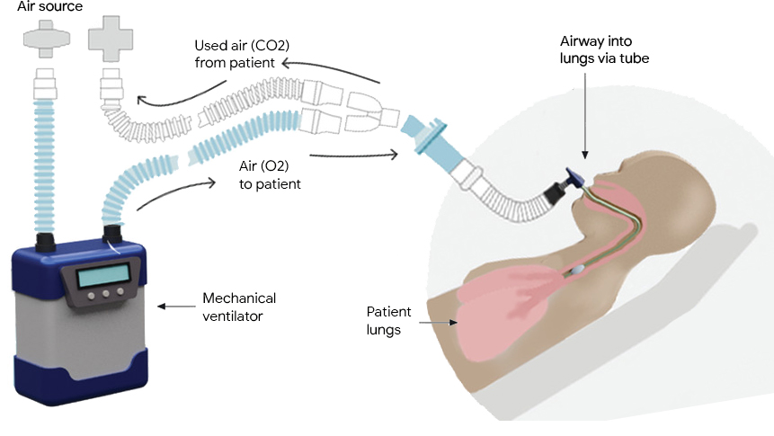A mechanical ventilator takes breaths for patients who are not fully capable of doing so on their own. In invasive ventilation, a controllable, compressed air source is connected to a sedated patient via tubing called a respiratory circuit.

In both invasive and non-invasive ventilation, the ventilator follows a clinician-prescribed breathing waveform based on a respiratory measurement from the patient (e.g., airway pressure, tidal volume). In order to prevent harm, this demanding task requires both robustness to differences or changes in patients' lungs and adherence to the desired waveform. Consequently, ventilators require significant attention from highly-trained clinicians in order to ensure that their performance matches the patients’ needs and that they do not cause lung damage.

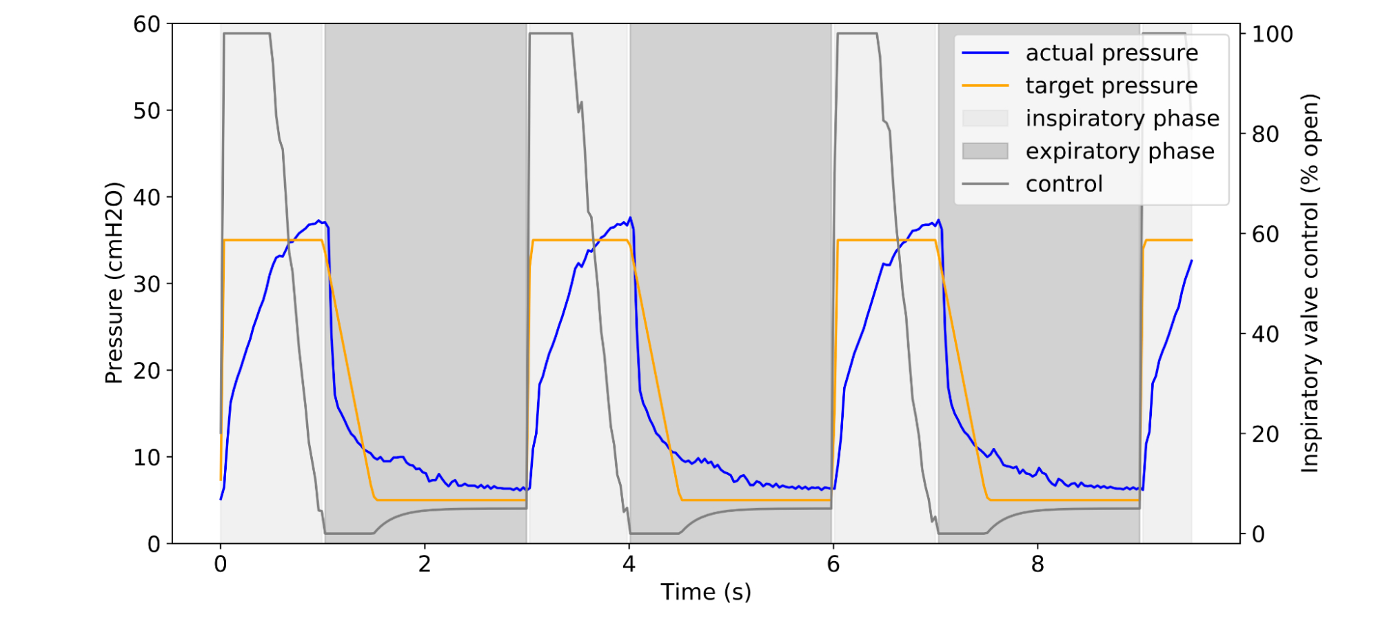Example of a clinician-prescribed breathing waveform (orange) in units of airway pressure and the actual pressure (blue), given some controller algorithm.

In “Machine Learning for Mechanical Ventilation Control”, we present exploratory research into the design of a deep learning–based algorithm to improve medical ventilator control for invasive ventilation. Using signals from an artificial lung, we design a control algorithm that measures airway pressure and computes necessary adjustments to the airflow to better and more consistently match prescribed values. Compared to other approaches, we demonstrate improved robustness and better performance while requiring less manual intervention from clinicians, which suggests that this approach could reduce the likelihood of harm to a patient’s lungs.

Current Methods
Today, ventilators are controlled with methods belonging to the PID family (i.e., Proportional, Integral, Differential), which control a system based on the history of errors between the observed and desired states. A PID controller uses three characteristics for ventilator control: proportion (“P”) — a comparison of the measured and target pressure; integral (“I”) — the sum of previous measurements; and differential (“D”) — the difference between two previous measurements. Variants of PID have been used since the 17th century and today form the basis of many controllers in both industrial (e.g., controlling heat or fluids) and consumer (e.g., controlling espresso pressure) applications.

PID control forms a solid baseline, relying on the sharp reactivity of P control to rapidly increase lung pressure when breathing in and the stability of I control to hold the breath in before exhaling. However, operators must tune the ventilator for specific patients, often repeatedly, to balance the “ringing” of overzealous P control against the ineffectually slow rise in lung pressure of dominant I control.

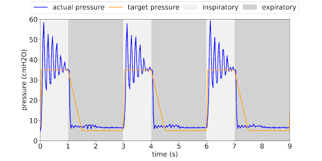Current PID methods are prone to over- and then under-shooting their target (ringing). Because patients differ in their physiology and may even change during treatment, highly-trained clinicians must constantly monitor and adjust existing methods to ensure such violent ringing as in the above example does not occur.

To more effectively balance these characteristics, we propose a neural network–based controller to create a set of control signals that are more broad and adaptable than PID-generated controls.

A Machine-Learned Ventilator Controller
While one could tune the coefficients of a PID controller (either manually or via an exhaustive grid search) through a limited number of repeated trials, it is impossible to apply such a direct approach towards a deep controller, as deep neural networks (DNNs) are often parameter-rich and require significant training data. Similarly, popular model-free approaches, such as Q-Learning or Policy Gradient, are data-intensive and therefore unsuitable for the physical system at hand. Further, these approaches don't take into account the intrinsic differentiability of the ventilator dynamical system, which is deterministic, continuous and contact-free.

We therefore adopt a model-based approach, where we first learn a DNN-based simulator of the ventilator-patient dynamical system. An advantage of learning such a simulator is that it provides a more accurate data-driven alternative to physics-based models, and can be more widely distributed for controller research.

To train a faithful simulator, we built a dataset by exploring the space of controls and the resulting pressures, while balancing against physical safety, e.g., not over-inflating a test lung and causing damage. Though PID control can exhibit ringing behavior, it performs well enough to use as a baseline for generating training data. To safely explore and to faithfully capture the behavior of the system, we use PID controllers with varied control coefficients to generate the control-pressure trajectory data for simulator training. Further, we add random deviations to the PID controllers to capture the dynamics more robustly.

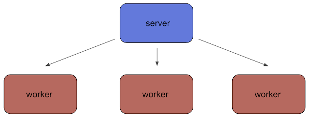
We collect data for training by running mechanical ventilation tasks on a physical test lung using an open-source ventilator designed by Princeton University's People's Ventilator Project. We built a ventilator farm housing ten ventilator-lung systems on a server rack, which captures multiple airway resistance and compliance settings that span a spectrum of patient lung conditions, as required for practical applications of ventilator systems.

We use a rack-based ventilator farm (10 ventilators / artificial lungs) to collect training data for a ventilator-lung simulator. Using this simulator, we train a DNN controller that we then validate on the physical ventilator farm.

The true underlying state of the dynamical system is not available to the model directly, but rather only through observations of the airway pressure in the system. In the simulator we model the state of the system at any time as a collection of previous pressure observations and the control actions applied to the system (up to a limited lookback window). These inputs are fed into a DNN that predicts the subsequent pressure in the system. We train this simulator on the control-pressure trajectory data collected through interactions with the test lung.

The performance of the simulator is measured via the sum of deviations of the simulator’s predictions (under self-simulation) from the ground truth.

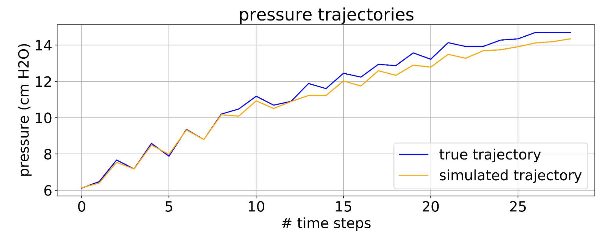While it is infeasible to compare real dynamics with their simulated counterparts over all possible trajectories and control inputs, we measure the distance between simulation and the known safe trajectories. We introduce some random exploration around these safe trajectories for robustness.

Having learned an accurate simulator, we then use it to train a DNN-based controller completely offline. This approach allows us to rapidly apply updates during controller training. Furthermore, the differentiable nature of the simulator allows for the stable use of the direct policy gradient, where we analytically compute the gradient of the loss with respect to the DNN parameters. We find this method to be significantly more efficient than model-free approaches.

Results
To establish a baseline, we run an exhaustive grid of PID controllers for multiple lung settings and select the best performing PID controller as measured by average absolute deviation between the desired pressure waveform and the actual pressure waveform. We compare these to our controllers and provide evidence that our DNN controllers are better performing and more robust.

Breathing waveform tracking performance:

We compare the best PID controller for a given lung setting against our controller trained on the learned simulator for the same setting. Our learned controller shows a 22% lower mean absolute error (MAE) between target and actual pressure waveforms.

Comparison of the MAE between target and actual pressure waveforms (lower is better) for the best PID controller (orange) for a given lung setting (shown for two settings, R=5 and R=20) against our controller (blue) trained on the learned simulator for the same setting. The learned controller performs up to 22% better.

Robustness:

Further, we compare the performance of the single best PID controller across the entire set of lung settings with our controller trained on a set of learned simulators over the same settings. Our controller performs up to 32% better in MAE between target and actual pressure waveforms, suggesting that it could require less manual intervention between patients or even as a patient's condition changes.

As above, but comparing the single best PID controller across the entire set of lung settings against our controller trained over the same settings. The learned controller performs up to 32% better, suggesting that it may require less manual intervention.

Finally, we investigated the feasibility of using model-free and other popular RL algorithms (PPO, DQN), in comparison to a direct policy gradient trained on the simulator. We find that the simulator-trained direct policy gradient achieves slightly better scores and does so with a more stable training process that uses orders of magnitude fewer training samples and a significantly smaller hyperparameter search space.

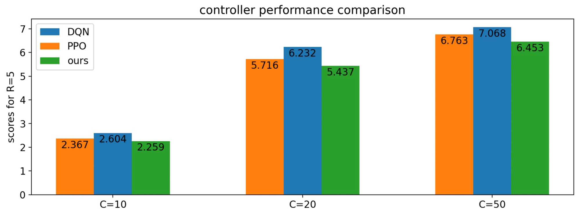In the simulator, we find that model-free and other popular algorithms (PPO, DQN) perform approximately as well as our method.

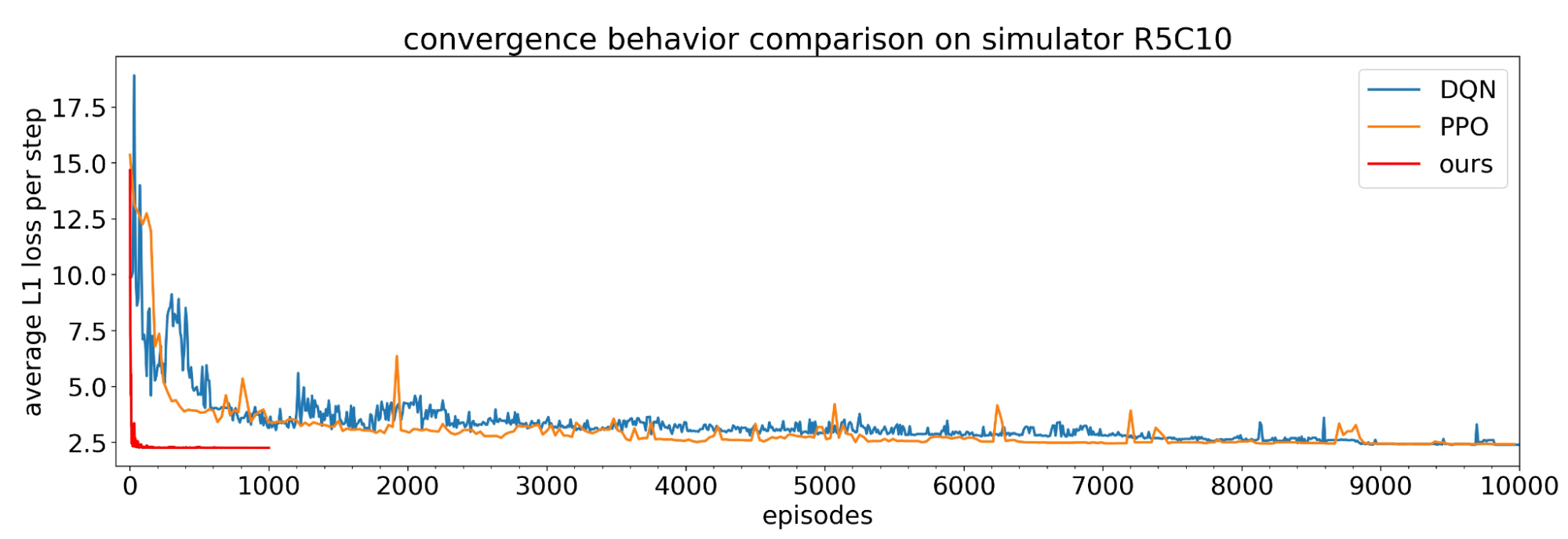However, these other methods take an order of magnitude more episodes to train to similar levels.

Conclusions and the Road Forward
We have described a deep-learning approach to mechanical ventilation based on simulated dynamics learned from a physical test lung. However, this is only the beginning. To make an impact on real-world ventilators there are numerous other considerations and issues to take into account. Most important amongst them are non-invasive ventilators, which are significantly more challenging due to the difficulty of discerning pressure from lungs and mask pressure. Other directions are how to handle spontaneous breathing and coughing. To learn more and become involved in this important intersection of machine learning and health, see an ICML tutorial on control theory and learning, and consider participating in one of our kaggle competitions for creating better ventilator simulators!

Acknowledgements
The primary work was based in the Google AI Princeton lab, in collaboration with Cohen lab at the Mechanical and Aerospace Engineering department at Princeton University. The research paper was authored by contributors from Google and Princeton University, including: Daniel Suo, Naman Agarwal, Wenhan Xia, Xinyi Chen, Udaya Ghai, Alexander Yu, Paula Gradu, Karan Singh, Cyril Zhang, Edgar Minasyan, Julienne LaChance, Tom Zajdel, Manuel Schottdorf, Daniel Cohen, and Elad Hazan.

Source: Google AI Blog

Good News About the Carbon Footprint of Machine Learning Training

Posted by David Patterson, Distinguished Engineer, Google Research, Brain Team

Machine learning (ML) has become prominent in information technology, which has led some to raise concerns about the associated rise in the costs of computation, primarily the carbon footprint, i.e., total greenhouse gas emissions. While these assertions rightfully elevated the discussion around carbon emissions in ML, they also highlight the need for accurate data to assess true carbon footprint, which can help identify strategies to mitigate carbon emission in ML.

In “The Carbon Footprint of Machine Learning Training Will Plateau, Then Shrink”, accepted for publication in IEEE Computer, we focus on operational carbon emissions — i.e., the energy cost of operating ML hardware, including data center overheads — from training of natural language processing (NLP) models and investigate best practices that could reduce the carbon footprint. We demonstrate four key practices that reduce the carbon (and energy) footprint of ML workloads by large margins, which we have employed to help keep ML under 15% of Google’s total energy use.

The 4Ms: Best Practices to Reduce Energy and Carbon Footprints
We identified four best practices that reduce energy and carbon emissions significantly — we call these the “4Ms” — all of which are being used at Google today and are available to anyone using Google Cloud services.

Model. Selecting efficient ML model architectures, such as sparse models, can advance ML quality while reducing computation by 3x–10x.
Machine. Using processors and systems optimized for ML training, versus general-purpose processors, can improve performance and energy efficiency by 2x–5x.
Mechanization. Computing in the Cloud rather than on premise reduces energy usage and therefore emissions by 1.4x–2x. Cloud-based data centers are new, custom-designed warehouses equipped for energy efficiency for 50,000 servers, resulting in very good power usage effectiveness (PUE). On-premise data centers are often older and smaller and thus cannot amortize the cost of new energy-efficient cooling and power distribution systems.
Map Optimization. Moreover, the cloud lets customers pick the location with the cleanest energy, further reducing the gross carbon footprint by 5x–10x. While one might worry that map optimization could lead to the greenest locations quickly reaching maximum capacity, user demand for efficient data centers will result in continued advancement in green data center design and deployment.

These four practices together can reduce energy by 100x and emissions by 1000x.

Note that Google matches 100% of its operational energy use with renewable energy sources. Conventional carbon offsets are usually retrospective up to a year after the carbon emissions and can be purchased anywhere on the same continent. Google has committed to decarbonizing all energy consumption so that by 2030, it will operate on 100% carbon-free energy, 24 hours a day on the same grid where the energy is consumed. Some Google data centers already operate on 90% carbon-free energy; the overall average was 61% carbon-free energy in 2019 and 67% in 2020.

Below, we illustrate the impact of improving the 4Ms in practice. Other studies examined training the Transformer model on an Nvidia P100 GPU in an average data center and energy mix consistent with the worldwide average. The recently introduced Primer model reduces the computation needed to achieve the same accuracy by 4x. Using newer-generation ML hardware, like TPUv4, provides an additional 14x improvement over the P100, or 57x overall. Efficient cloud data centers gain 1.4x over the average data center, resulting in a total energy reduction of 83x. In addition, using a data center with a low-carbon energy source can reduce the carbon footprint another 9x, resulting in a 747x total reduction in carbon footprint over four years.

Reduction in gross carbon dioxide equivalent emissions (CO₂e) from applying the 4M best practices to the Transformer model trained on P100 GPUs in an average data center in 2017, as done in other studies. Displayed values are the cumulative improvement successively addressing each of the 4Ms: updating the model to Primer; upgrading the ML accelerator to TPUv4; using a Google data center with better PUE than average; and training in a Google Oklahoma data center that uses very clean energy.

Overall Energy Consumption for ML
Google’s total energy usage increases annually, which is not surprising considering increased use of its services. ML workloads have grown rapidly, as has the computation per training run, but paying attention to the 4Ms — optimized models, ML-specific hardware, efficient data centers — has largely compensated for this increased load. Our data shows that ML training and inference are only 10%–15% of Google’s total energy use for each of the last three years, each year split ⅗ for inference and ⅖ for training.

Prior Emission Estimates
Google uses neural architecture search (NAS) to find better ML models. NAS is typically performed once per problem domain/search space combination, and the resulting model can then be reused for thousands of applications — e.g., the Evolved Transformer model found by NAS is open sourced for all to use. As the optimized model found by NAS is often more efficient, the one time cost of NAS is typically more than offset by emission reductions from subsequent use.

A study from the University of Massachusetts (UMass) estimated carbon emissions for the Evolved Transformer NAS.

Without ready access to Google hardware or data centers, the study extrapolated from the available P100 GPUs instead of TPUv2s, and assumed US average data center efficiency instead of highly efficient hyperscale data centers. These assumptions increased the estimate by 5x over the energy used by the actual NAS computation that was performed in Google’s data center.
In order to accurately estimate the emissions for NAS, it's important to understand the subtleties of how they work. NAS systems use a much smaller proxy task to search for the most efficient models to save time, and then scale up the found models to full size. The UMass study assumed that the search repeated full size model training thousands of times, resulting in emission estimates that are another 18.7x too high.

The overshoot for the NAS was 88x: 5x for energy-efficient hardware in Google data centers and 18.7x for computation using proxies. The actual CO₂e for the one-time search were 3,223 kg versus 284,019 kg, 88x less than the published estimate.

Unfortunately, some subsequent papers misinterpreted the NAS estimate as the training cost for the model it discovered, yet emissions for this particular NAS are ~1300x larger than for training the model. These papers estimated that training the Evolved Transformer model takes two million GPU hours, costs millions of dollars, and that its carbon emissions are equivalent to five times the lifetime emissions of a car. In reality, training the Evolved Transformer model on the task examined by the UMass researchers and following the 4M best practices takes 120 TPUv2 hours, costs $40, and emits only 2.4 kg (0.00004 car lifetimes), 120,000x less. This gap is nearly as large as if one overestimated the CO₂e to manufacture a car by 100x and then used that number as the CO₂e for driving a car.

Outlook
Climate change is important, so we must get the numbers right to ensure that we focus on solving the biggest challenges. Within information technology, we believe these are much more likely the lifecycle costs — i.e., emission estimates that include the embedded carbon emitted from manufacturing all components involved, from chips to data center buildings — of manufacturing computing equipment of all types and sizes¹ rather than the operational cost of ML training.

Expect more good news if everyone improves the 4Ms. While these numbers may currently vary across companies, these simple measures can be followed across the industry:

Data center providers should publish data center efficiency and the cleanliness of the energy supply per location so that customers can understand and reduce their energy consumption and carbon footprint.
ML practitioners should train models using the best processors in the greenest data centers, which today are often in the Cloud.
ML researchers should continue to develop more efficient ML models, for example, by leveraging sparsity or by integrating retrieval to shrink the model. They should also publish energy consumption and carbon footprint, both to foster competition beyond model quality and to ensure accurate accounting of their work, which is difficult to do accurately post-hoc.

If the 4Ms become widely recognized, we predict a virtuous circle that will bend the curve so that the global carbon footprint of ML training is actually shrinking, not increasing.

Acknowledgements
Let me thank my co-authors who stayed with this long and winding investigation into a topic that was new to most of us: Jeff Dean, Joseph Gonzalez, Urs Hölzle, Quoc Le, Chen Liang, Lluis-Miquel Munguia, Daniel Rothchild, David So, and Maud Texier. We also had a great deal of help from others along the way for an earlier study that eventually led to this version of the paper. Emma Strubell made several suggestions for the prior paper, including the recommendation to examine the recent giant NLP models. Christopher Berner, Ilya Sutskever, OpenAI, and Microsoft shared information about GPT-3. Dmitry Lepikhin and Zongwei Zhou did a great deal of work to measure the performance and power of GPUs and TPUs in Google data centers. Hallie Cramer, Anna Escuer, Elke Michlmayr, Kelli Wright, and Nick Zakrasek helped with the data and policies for energy and CO₂e emissions at Google.

¹Worldwide IT manufacturing for 2021 included 1700M cell phones, 340M PCs, and 12M data center servers. ^↩

Source: Google AI Blog

Nested Hierarchical Transformer: Towards Accurate, Data-Efficient, and Interpretable Visual Understanding

Posted by Zizhao Zhang, Software Engineer, Google Research, Cloud AI Team

In visual understanding, the Visual Transformer (ViT) and its variants have received significant attention recently due to their superior performance on many core visual applications, such as image classification, object detection, and video understanding. The core idea of ViT is to utilize the power of self-attention layers to learn global relationships between small patches of images. However, the number of connections between patches increases quadratically with image size. Such a design has been observed to be data inefficient — although the original ViT can perform better than convolutional networks with hundreds of millions of images for pre-training, such a data requirement is not always practical, and it still underperforms compared to convolutional networks when given less data. Many are exploring to find more suitable architectural re-designs that can learn visual representations effectively, such as by adding convolutional layers and building hierarchical structures with local self-attention.

The principle of hierarchical structure is one of the core ideas in vision models, where bottom layers learn more local object structures on the high-dimensional pixel space and top layers learn more abstracted and high-level knowledge at low-dimensional feature space. Existing ViT-based methods focus on designing a variety of modifications inside self-attention layers to achieve such a hierarchy, but while these offer promising performance improvements, they often require substantial architectural re-designs. Moreover, these approaches lack an interpretable design, so it is difficult to explain the inner-workings of trained models.

To address these challenges, in “Nested Hierarchical Transformer: Towards Accurate, Data-Efficient and Interpretable Visual Understanding”, we present a rethinking of existing hierarchical structure–driven designs, and provide a novel and orthogonal approach to significantly simplify them. The central idea of this work is to decouple feature learning and feature abstraction (pooling) components: nested transformer layers encode visual knowledge of image patches separately, and then the processed information is aggregated. This process is repeated in a hierarchical manner, resulting in a pyramid network structure. The resulting architecture achieves competitive results on ImageNet and outperforms results on data-efficient benchmarks. We have shown such a design can meaningfully improve data efficiency with faster convergence and provide valuable interpretability benefits. Moreover, we introduce GradCAT, a new technique for interpreting the decision process of a trained model at inference time.

Architecture Design
The overall architecture is simple to implement by adding just a few lines of Python code to the source code of the original ViT. The original ViT architecture divides an input image into small patches, projects pixels of each patch to a vector with predefined dimension, and then feeds the sequences of all vectors to the overall ViT architecture containing multiple stacked identical transformer layers. While every layer in ViT processes information of the whole image, with this new method, stacked transformer layers are used to process only a region (i.e., block) of the image containing a few spatially adjacent image patches. This step is independent for each block and is also where feature learning occurs. Finally, a new computational layer called block aggregation then combines all of the spatially adjacent blocks. After each block aggregation, the features corresponding to four spatially adjacent blocks are fed to another module with a stack of transformer layers, which then process those four blocks jointly. This design naturally builds a pyramid hierarchical structure of the network, where bottom layers can focus on local features (such as textures) and upper layers focus on global features (such as object shape) at reduced dimensionality thanks to the block aggregation.

A visualization of the network processing an image: Given an input image, the network first partitions images into blocks, where each block contains 4 image patches. Image patches in every block are linearly projected as vectors and processed by a stack of identical transformer layers. Then the proposed block aggregation layer aggregates information from each block and reduces its spatial size by 4 times. The number of blocks is reduced to 1 at the top hierarchy and classification is conducted after the output of it.

Interpretability
This architecture has a non-overlapping information processing mechanism, independent at every node. This design resembles a decision tree-like structure, which manifests unique interpretability capabilities because every tree node contains independent information of an image block that is being received by its parent nodes. We can trace the information flow through the nodes to understand the importance of each feature. In addition, our hierarchical structure retains the spatial structure of images throughout the network, leading to learned spatial feature maps that are effective for interpretation. Below we showcase two kinds of visual interpretability.

First, we present a method to interpret the trained model on test images, called gradient-based class-aware tree-traversal (GradCAT). GradCAT traces the feature importance of each block (a tree node) from top to bottom of the hierarchy structure. The main idea is to find the most valuable traversal from the root node at the top layer to a child node at the bottom layer that contributes the most to the classification outcomes. Since each node processes information from a certain region of the image, such traversal can be easily mapped to the image space for interpretation (as shown by the overlaid dots and lines in the image below).

The following is an example of the model's top-4 predictions and corresponding interpretability results on the left input image (containing 4 animals). As shown below, GradCAT highlights the decision path along the hierarchical structure as well as the corresponding visual cues in local image regions on the images.

Given the left input image (containing four objects), the figure visualizes the interpretability results of the top-4 prediction classes. The traversal locates the model decision path along the tree and simultaneously locates the corresponding image patch (shown by the dotted line on images) that has the highest impact to the predicted target class.

Moreover, the following figures visualize results on the ImageNet validation set and show how this approach enables some intuitive observations. For instance, the example of the lighter below (upper left panel) is particularly interesting because the ground truth class — lighter/matchstick — actually defines the bottom-right matchstick object, while the most salient visual features (with the highest node values) are actually from the upper-left red light, which conceptually shares visual cues with a lighter. This can also be seen from the overlaid red lines, which indicate the image patches with the highest impact on the prediction. Thus, although the visual cue is a mistake, the output prediction is correct. In addition, the four child nodes of the wooden spoon below have similar feature importance values (see numbers visualized in the nodes; higher indicates more importance), which is because the wooden texture of the table is similar to that of the spoon.

Visualization of the results obtained by the proposed GradCAT. Images are from the ImageNet validation dataset.

Second, different from the original ViT, our hierarchical architecture retains spatial relationships in learned representations. The top layers output low-resolution features maps of input images, enabling the model to easily perform attention-based interpretation by applying Class Attention Map (CAM) on the learned representations at the top hierarchical level. This enables high-quality weakly-supervised object localization with just image-level labels. See the following figure for examples.

Visualization of CAM-based attention results. Warmer colors indicate higher attention. Images are from the ImageNet validation dataset.

Convergence Advantages
With this design, feature learning only happens at local regions independently, and feature abstraction happens inside the aggregation function. This design and simple implementation is general enough for other types of visual understanding tasks beyond classification. It also improves the model convergence speed greatly, significantly reducing the training time to reach the desired maximum accuracy.

We validate this advantage in two ways. First, we compare the ViT structure on the ImageNet accuracy with a different number of total training epochs. The results are shown on the left side of the figure below, demonstrating much faster convergence than the original ViT, e.g., around 20% improvement in accuracy over ViT with 30 total training epochs.

Second, we modify the architecture to conduct unconditional image generation tasks, since training ViT-based models for image generation tasks is challenging due to convergence and speed issues. Creating such a generator is straightforward by transposing the proposed architecture: the input is an embedding vector, the output is a full image in RGB channels, and the block aggregation is replaced by a block de-aggregation component supported by Pixel Shuffling. Surprisingly, we find our generator is easy to train and demonstrates faster convergence speed, as well as better FID score (which measures how similar generated images are to real ones), than the capacity-comparable SAGAN.

Left: ImageNet accuracy given different number of total training epochs compared with standard ViT architecture. Right: ImageNet 64x64 image generation FID scores (lower is better) with single 1000-epoch training. On both tasks, our method shows better convergence speed.

Conclusion
In this work we demonstrate the simple idea that decoupled feature learning and feature information extraction in this nested hierarchy design leads to better feature interpretability through a new gradient-based class-aware tree traversal method. Moreover, the architecture improves convergence on not only classification tasks but also image generation tasks. The proposed idea is focusing on aggregation function and thereby is orthogonal to advanced architecture design for self-attention. We hope this new research encourages future architecture designers to explore more interpretable and data-efficient ViT-based models for visual understanding, like the adoption of this work for high-resolution image generation. We have also released the source code for the image classification portion of this work.

Acknowledgements
We gratefully acknowledge the contributions of other co-authors, including Han Zhang, Long Zhao, Ting Chen, Sercan Arik, Tomas Pfister. We also thank Xiaohua Zhai, Jeremy Kubica, Kihyuk Sohn, and Madeleine Udell for the valuable feedback of the work.

Source: Google AI Blog

Nested Hierarchical Transformer: Towards Accurate, Data-Efficient, and Interpretable Visual Understanding

Posted by Zizhao Zhang, Software Engineer, Google Research, Cloud AI Team

Visualization of the results obtained by the proposed GradCAT. Images are from the ImageNet validation dataset.

Visualization of CAM-based attention results. Warmer colors indicate higher attention. Images are from the ImageNet validation dataset.

Source: Google AI Blog

Scaling Vision with Sparse Mixture of Experts

Posted by Carlos Riquelme, Research Scientist and Joan Puigcerver, Software Engineer, Google Research, Brain team

Advances in deep learning over the last few decades have been driven by a few key elements. With a small number of simple but flexible mechanisms (i.e., inductive biases such as convolutions or sequence attention), increasingly large datasets, and more specialized hardware, neural networks can now achieve impressive results on a wide range of tasks, such as image classification, machine translation, and protein folding prediction.

However, the use of large models and datasets comes at the expense of significant computational requirements. Yet, recent works suggest that large model sizes might be necessary for strong generalization and robustness, so training large models while limiting resource requirements is becoming increasingly important. One promising approach involves the use of conditional computation: rather than activating the whole network for every single input, different parts of the model are activated for different inputs. This paradigm has been featured in the Pathways vision and recent works on large language models, while it has not been well explored in the context of computer vision.

In “Scaling Vision with Sparse Mixture of Experts”, we present V-MoE, a new vision architecture based on a sparse mixture of experts, which we then use to train the largest vision model to date. We transfer V-MoE to ImageNet and demonstrate matching state-of-the-art accuracy while using about 50% fewer resources than models of comparable performance. We have also open-sourced the code to train sparse models and provided several pre-trained models.

Vision Mixture of Experts (V-MoEs)
Vision Transformers (ViT) have emerged as one of the best architectures for vision tasks. ViT first partitions an image into equally-sized square patches. These are called tokens, a term inherited from language models. Still, compared to the largest language models, ViT models are several orders of magnitude smaller in terms of number of parameters and compute.

To massively scale vision models, we replace some dense feedforward layers (FFN) in the ViT architecture with a sparse mixture of independent FFNs (which we call experts). A learnable router layer selects which experts are chosen (and how they are weighted) for every individual token. That is, different tokens from the same image may be routed to different experts. Each token is only routed to at most K (typically 1 or 2) experts, among a total of E experts (in our experiments, E is typically 32). This allows scaling the model’s size while keeping its computation per token roughly constant. The figure below shows the structure of the encoder blocks in more detail.

V-MoE Transformer Encoder block.

Experimental Results
We first pre-train the model once on JFT-300M, a large dataset of images. The left plot below shows our pre-training results for models of all sizes: from the small S/32 to the huge H/14.

We then transfer the model to new downstream tasks (such as ImageNet), by using a new head (the last layer in a model). We explore two transfer setups: either fine-tuning the entire model on all available examples of the new task, or freezing the pre-trained network and tuning only the new head using a few examples (known as few-shot transfer). The right plot in the figure below summarizes our transfer results to ImageNet, training on only 5 images per class (called 5-shot transfer).

JFT-300M Precision@1 and ImageNet 5-shot accuracy. Colors represent different ViT variants and markers represent either standard ViT (●), or V-MoEs (▸) with expert layers on the last n even blocks. We set n=2 for all models, except V-MoE-H where n=5. Higher indicates better performance, with more efficient models being to the left.

In both cases, the sparse model strongly outperforms its dense counterpart at a given amount of training compute (shown by the V-MoE line being above the ViT line), or achieves similar performance much faster (shown by the V-MoE line being to the left of the ViT line).

To explore the limits of vision models, we trained a 15-billion parameter model with 24 MoE layers (out of 48 blocks) on an extended version of JFT-300M. This massive model — the largest to date in vision as far as we know — achieved 90.35% test accuracy on ImageNet after fine-tuning, near the current state-of-the-art.

Priority Routing
In practice, due to hardware constraints, it is not efficient to use buffers with a dynamic size, so models typically use a pre-defined buffer capacity for each expert. Assigned tokens beyond this capacity are dropped and not processed once the expert becomes "full". As a consequence, higher capacities yield higher accuracy, but they are also more computationally expensive.

We leverage this implementation constraint to make V-MoEs faster at inference time. By decreasing the total combined buffer capacity below the number of tokens to be processed, the network is forced to skip processing some tokens in the expert layers. Instead of choosing the tokens to skip in some arbitrary fashion (as previous works did), the model learns to sort tokens according to an importance score. This maintains high quality predictions while saving a lot of compute. We refer to this approach as Batch Priority Routing (BPR), illustrated below.

Under high capacity, both vanilla and priority routing work well as all patches are processed. However, when the buffer size is reduced to save compute, vanilla routing selects arbitrary patches to process, often leading to poor predictions. BPR smartly prioritizes important patches resulting in better predictions at lower computational costs.

Dropping the right tokens turns out to be essential to deliver high-quality and more efficient inference predictions. When the expert capacity decreases, performance quickly decreases with the vanilla routing mechanism. Conversely, BPR is much more robust to low capacities.

Performance versus inference capacity buffer size (or ratio) C for a V-MoE-H/14 model with K=2. Even for large C’s, BPR improves performance; at low C the difference is quite significant. BPR is competitive with dense models (ViT-H/14) by processing only 15-30% of the tokens.

Overall, we observed that V-MoEs are highly flexible at inference time: for instance, one can decrease the number of selected experts per token to save time and compute, without any further training on the model weights.

Exploring V-MoEs
Because much is yet to be discovered about the internal workings of sparse networks, we also explored the routing patterns of the V-MoE.

One hypothesis is that routers would learn to discriminate and assign tokens to experts based on some semantic grounds (the “car” expert, the “animal” experts, and so on). To test this, below we show plots for two different MoE layers (a very early-on one, and another closer to the head). The x-axis corresponds to each of the 32 experts, and the y-axis shows the ID of the image classes (from 1 to 1000). Each entry in the plot shows how often an expert was selected for tokens corresponding to the specific image class, with darker colors indicating higher frequency. While in the early layers there is little correlation, later in the network, each expert receives and processes tokens from only a handful of classes. Therefore, we can conclude that some semantic clustering of the patches emerges in the deeper layers of the network.

Higher routing decisions correlate with image classes. We show two MoE layers of a V-MoE-H/14. The x-axis corresponds to the 32 experts in a layer. The y-axis are the 1000 ImageNet classes; orderings for both axes are different across plots (to highlight correlations). For each pair (expert e, class c) we show the average routing weight for the tokens corresponding to all images with class c for that particular expert e.

Final Thoughts
We train very large vision models using conditional computation, delivering significant improvements in representation and transfer learning for relatively little training cost. Alongside V-MoE, we introduced BPR, which requires the model to process only the most useful tokens in the expert layers.

We believe this is just the beginning of conditional computation at scale for computer vision; extensions include multi-modal and multi-task models, scaling up the expert count, and improving transfer of the representations produced by sparse models. Heterogeneous expert architectures and conditional variable-length routes are also promising directions. Sparse models can especially help in data rich domains such as large-scale video modeling. We hope our open-source code and models help attract and engage researchers new to this field.

Acknowledgments
We thank our co-authors: Basil Mustafa, Maxim Neumann, Rodolphe Jenatton, André Susano Pinto, Daniel Keysers, and Neil Houlsby. We thank Alex Kolesnikov, Lucas Beyer, and Xiaohua Zhai for providing continuous help and details about scaling ViT models. We are also grateful to Josip Djolonga, Ilya Tolstikhin, Liam Fedus, and Barret Zoph for feedback on the paper; James Bradbury, Roy Frostig, Blake Hechtman, Dmitry Lepikhin, Anselm Levskaya, and Parker Schuh for invaluable support helping us run our JAX models efficiently on TPUs; and many others from the Brain team for their support. Finally, we would also like to thank and acknowledge Tom Small for the awesome animated figure used in this post.

Source: Google AI Blog

Prediction Framework, a time saver for Data Science prediction projects

Posted by Álvaro Lamas, Héctor Parra, Jaime Martínez, Julia Hernández, Miguel Fernandes, Pablo Gil

Acquiring high value customers using predicted Lifetime Value, taking specific actions on high propensity of churn users, generating and activating audiences based on machine learning processed signals…All of those marketing scenarios require of analyzing first party data, performing predictions on the data and activating the results into the different marketing platforms like Google Ads as frequently as possible to keep the data fresh.

Feeding marketing platforms like Google Ads on a regular and frequent basis, requires a robust, report oriented and cost reduced ETL & prediction pipeline. These pipelines are very similar regardless of the use case and it’s very easy to fall into reinventing the wheel every time or manually copy & paste structural code increasing the risk of introducing errors.

Wouldn't it be great to have a common reusable structure and just add the specific code for each of the stages?

Here is where Prediction Framework plays a key role in helping you implement and accelerate your first-party data prediction projects by providing the backbone elements of the predictive process.

Prediction Framework is a fully customizable pipeline that allows you to simplify the implementation of prediction projects. You only need to have the input data source, the logic to extract and process the data and a Vertex AutoML model ready to use along with the right feature list, and the framework will be in charge of creating and deploying the required artifacts. With a simple configuration, all the common artifacts of the different stages of this type of projects will be created and deployed for you: data extraction, data preparation (aka feature engineering), filtering, prediction and post-processing, in addition to some other operational functionality including backfilling, throttling (for API limits), synchronization, storage and reporting.

The Prediction Framework was built to be hosted in the Google Cloud Platform and it makes use of Cloud Functions to do all the data processing (extraction, preparation, filtering and post-prediction processing), Firestore, Pub/Sub and Schedulers for the throttling system and to coordinate the different phases of the predictive process, Vertex AutoML to host your machine learning model and BigQuery as the final storage of your predictions.

Prediction Framework Architecture

To get involved and start using the Prediction Framework, a configuration file needs to be prepared with some environment variables about the Google Cloud Project to be used, the data sources, the ML model to make the predictions and the scheduler for the throttling system. In addition, custom queries for the data extraction, preparation, filtering and post-processing need to be added in the deploy files customization. Then, the deployment is done automatically using a deployment script provided by the tool.

Once deployed, all the stages will be executed one after the other, storing the intermediate and final data in the BigQuery tables:

Extract: this step will, on a timely basis, query the transactions from the data source, corresponding to the run date (scheduler or backfill run date) and will store them in a new table into the local project BigQuery.
Prepare: immediately after the extract of the transactions for one specific date is available, the data will be picked up from the local BigQuery and processed according to the specs of the model. Once the data is processed, it will be stored in a new table into the local project BigQuery.
Filter: this step will query the data stored by the prepare process and will filter the required data and store it into the local project BigQuery. (i.e only taking into consideration new customers transactionsWhat a new customer is up to the instantiation of the framework for the specific use case. Will be covered later).
Predict: once the new customers are stored, this step will read them from BigQuery and call the prediction using Vertex API. A formula based on the result of the prediction could be applied to tune the value or to apply thresholds. Once the data is ready, it will be stored into the BigQuery within the target project.
Post_process: A formula could be applied to the AutoML batch results to tune the value or to apply thresholds. Once the data is ready, it will be stored into the BigQuery within the target project.

One of the powerful features of the prediction framework is that it allows backfilling directly from the BigQuery user interface, so in case you’d need to reprocess a whole period of time, it could be done in literally 4 clicks.

In summary: Prediction Framework simplifies the implementation of first-party data prediction projects, saving time and minimizing errors of manual deployments of recurrent architectures.

For additional information and to start experimenting, you can visit the Prediction Framework repository on Github.

Source: Google Developers Blog

Prediction Framework, a time saver for Data Science prediction projects

Posted by Álvaro Lamas, Héctor Parra, Jaime Martínez, Julia Hernández, Miguel Fernandes, Pablo Gil

Wouldn't it be great to have a common reusable structure and just add the specific code for each of the stages?

Here is where Prediction Framework plays a key role in helping you implement and accelerate your first-party data prediction projects by providing the backbone elements of the predictive process.

Prediction Framework Architecture

Once deployed, all the stages will be executed one after the other, storing the intermediate and final data in the BigQuery tables:

Extract: this step will, on a timely basis, query the transactions from the data source, corresponding to the run date (scheduler or backfill run date) and will store them in a new table into the local project BigQuery.
Prepare: immediately after the extract of the transactions for one specific date is available, the data will be picked up from the local BigQuery and processed according to the specs of the model. Once the data is processed, it will be stored in a new table into the local project BigQuery.
Filter: this step will query the data stored by the prepare process and will filter the required data and store it into the local project BigQuery. (i.e only taking into consideration new customers transactionsWhat a new customer is up to the instantiation of the framework for the specific use case. Will be covered later).
Predict: once the new customers are stored, this step will read them from BigQuery and call the prediction using Vertex API. A formula based on the result of the prediction could be applied to tune the value or to apply thresholds. Once the data is ready, it will be stored into the BigQuery within the target project.
Post_process: A formula could be applied to the AutoML batch results to tune the value or to apply thresholds. Once the data is ready, it will be stored into the BigQuery within the target project.

In summary: Prediction Framework simplifies the implementation of first-party data prediction projects, saving time and minimizing errors of manual deployments of recurrent architectures.

For additional information and to start experimenting, you can visit the Prediction Framework repository on Github.

Source: Google Developers Blog

Training Machine Learning Models More Efficiently with Dataset Distillation

Posted by Timothy Nguyen¹, Research Engineer and Jaehoon Lee, Senior Research Scientist, Google Research

For a machine learning (ML) algorithm to be effective, useful features must be extracted from (often) large amounts of training data. However, this process can be made challenging due to the costs associated with training on such large datasets, both in terms of compute requirements and wall clock time. The idea of distillation plays an important role in these situations by reducing the resources required for the model to be effective. The most widely known form of distillation is model distillation (a.k.a. knowledge distillation), where the predictions of large, complex teacher models are distilled into smaller models.

An alternative option to this model-space approach is dataset distillation [1, 2], in which a large dataset is distilled into a synthetic, smaller dataset. Training a model with such a distilled dataset can reduce the required memory and compute. For example, instead of using all 50,000 images and labels of the CIFAR-10 dataset, one could use a distilled dataset consisting of only 10 synthesized data points (1 image per class) to train an ML model that can still achieve good performance on the unseen test set.

Top: Natural (i.e., unmodified) CIFAR-10 images. Bottom: Distilled dataset (1 image per class) on CIFAR-10 classification task. Using only these 10 synthetic images as training data, a model can achieve test set accuracy of ~51%.

In “Dataset Meta-Learning from Kernel Ridge Regression'', published in ICLR 2021, and “Dataset Distillation with Infinitely Wide Convolutional Networks”, presented at NeurIPS 2021, we introduce two novel dataset distillation algorithms, Kernel Inducing Points (KIP) and Label Solve (LS), which optimize datasets using the loss function arising from kernel regression (a classical machine learning algorithm that fits a linear model to features defined through a kernel). Applying the KIP and LS algorithms, we obtain very efficient distilled datasets for image classification, reducing the datasets to 1, 10, or 50 data points per class while still obtaining state-of-the-art results on a number of benchmark image classification datasets. Additionally, we are also excited to release our distilled datasets to benefit the wider research community.

Methodology
One of the key theoretical insights of deep neural networks (DNN) in recent years has been that increasing the width of DNNs results in more regular behavior that makes them easier to understand. As the width is taken to infinity, DNNs trained by gradient descent converge to the familiar and simpler class of models arising from kernel regression with respect to the neural tangent kernel (NTK), a kernel that measures input similarity by computing dot products of gradients of the neural network. Thanks to the Neural Tangents library, neural kernels for various DNN architectures can be computed in a scalable manner.

We utilized the above infinite-width limit theory of neural networks to tackle dataset distillation. Dataset distillation can be formulated as a two-stage optimization process: an “inner loop” that trains a model on learned data, and an “outer loop” that optimizes the learned data for performance on natural (i.e., unmodified) data. The infinite-width limit replaces the inner loop of training a finite-width neural network with a simple kernel regression. With the addition of a regularizing term, the kernel regression becomes a kernel ridge-regression (KRR) problem. This is a highly valuable outcome because the kernel ridge regressor (i.e., the predictor from the algorithm) has an explicit formula in terms of its training data (unlike a neural network predictor), which means that one can easily optimize the KRR loss function during the outer loop.

The original data labels can be represented by one-hot vectors, i.e., the true label is given a value of 1 and all other labels are given values of 0. Thus, an image of a cat would have the label “cat” assigned a 1 value, while the labels for “dog” and “horse” would be 0. The labels we use involve a subsequent mean-centering step, where we subtract the reciprocal of the number of classes from each component (so 0.1 for 10-way classification) so that the expected value of each label component across the dataset is normalized to zero.

While the labels for natural images appear in this standard form, the labels for our learned distilled datasets are free to be optimized for performance. Having obtained the kernel ridge regressor from the inner loop, the KRR loss function in the outer loop computes the mean-square error between the original labels of natural images and the labels predicted by the kernel ridge regressor. KIP optimizes the support data (images and possibly labels) by minimizing the KRR loss function through gradient-based methods. The Label Solve algorithm directly solves for the set of support labels that minimizes the KRR loss function, generating a unique dense label vector for each (natural) support image.

Example of labels obtained by label solving. Left and Middle: Sample images with possible labels listed below. The raw, one-hot label is shown in blue and the final LS generated dense label is shown in orange. Right: The covariance matrix between original labels and learned labels. Here, 500 labels were distilled from the CIFAR-10 dataset. A test accuracy of 69.7% is achieved using these labels for kernel ridge-regression.

Distributed Computation
For simplicity, we focus on architectures that consist of convolutional neural networks with pooling layers. Specifically, we focus on the so-called “ConvNet” architecture and its variants because it has been featured in other dataset distillation studies. We used a slightly modified version of ConvNet that has a simple architecture given by three blocks of convolution, ReLu, and 2x2 average pooling and then a final linear readout layer, with an additional 3x3 convolution and ReLu layer prepended (see our GitHub for precise details).

ConvNet architecture used in DC/DSA. Ours has an additional 3x3 Conv and ReLu prepended.

To compute the neural kernels needed in our work, we used the Neural Tangents library.

The first stage of this work, in which we applied KRR, focused on fully-connected networks, whose kernel elements are cheap to compute. But a hurdle facing neural kernels for models with convolutional layers plus pooling is that the computation of each kernel element between two images scales as the square of the number of input pixels (due to the capturing of pixel-pixel correlations by the kernel). So, for the second stage of this work, we needed to distribute the computation of the kernel elements and their gradients across many devices.

Distributed computation for large scale metalearning.

We invoke a client-server model of distributed computation in which a server distributes independent workloads to a large pool of client workers. A key part of this is to divide the backpropagation step in a way that is computationally efficient (explained in detail in the paper).

We accomplish this using the open-source tools Courier (part of DeepMind’s Launchpad), which allows us to distribute computations across GPUs working in parallel, and JAX, for which novel usage of the jax.vjp function enables computationally efficient gradients. This distributed framework allows us to utilize hundreds of GPUs per distillation of the dataset, for both the KIP and LS algorithms. Given the compute required for such experiments, we are releasing our distilled datasets to benefit the wider research community.

Examples
Our first set of distilled images above used KIP to distill CIFAR-10 down to 1 image per class while keeping the labels fixed. Next, in the below figure, we compare the test accuracy of training on natural MNIST images, KIP distilled images with labels fixed, and KIP distilled images with labels optimized. We highlight that learning the labels provides an effective, albeit mysterious benefit to distilling datasets. Indeed the resulting set of images provides the best test performance (for infinite-width networks) despite being less interpretable.

MNIST dataset distillation with trainable and non-trainable labels. Top: Natural MNIST data. Middle: Kernel Inducing Point distilled data with fixed labels. Bottom: Kernel Inducing Point distilled data with learned labels.

Results
Our distilled datasets achieve state-of-the-art performance on benchmark image classification datasets, improving performance beyond previous state-of-the-art models that used convolutional architectures, Dataset Condensation (DC) and Dataset Condensation with Differentiable Siamese Augmentation (DSA). In particular, for CIFAR-10 classification tasks, a model trained on a dataset consisting of only 10 distilled data entries (1 image / class, 0.02% of the whole dataset) achieves a 64% test set accuracy. Here, learning labels and an additional image preprocessing step leads to a significant increase in performance beyond the 50% test accuracy shown in our first figure (see our paper for details). With 500 images (50 images / class, 1% of the whole dataset), the model reaches 80% test set accuracy. While these numbers are with respect to neural kernels (using the KRR infinite width limit), these distilled datasets can be used to train finite-width neural networks as well. In particular, for 10 data points on CIFAR-10, a finite-width ConvNet neural network achieves 50% test accuracy with 10 images and 68% test accuracy using 500 images, which are still state-of-the-art results. We provide a simple Colab notebook demonstrating this transfer to a finite-width neural network.

Dataset distillation using Kernel Inducing Points (KIP) with a convolutional architecture outperforms prior state-of-the-art models (DC/DSA) on all benchmark settings on image classification tasks. Label Solve (LS, middle columns) while only distilling information in the labels could often (e.g. CIFAR-10 10, 50 data points per class) outperform prior state-of-the-art models as well.

In some cases, our learned datasets are more effective than a natural dataset one hundred times larger in size.

Conclusion
We believe that our work on dataset distillation opens up many interesting future directions. For instance, our algorithms KIP and LS have demonstrated the effectiveness of using learned labels, an area that remains relatively underexplored. Furthermore, we expect that utilizing efficient kernel approximation methods can help to reduce computational burden and scale up to larger datasets. We hope this work encourages researchers to explore other applications of dataset distillation, including neural architecture search and continual learning, and even potential applications to privacy.

Anyone interested in the KIP and LS learned datasets for further analysis is encouraged to check out our papers [ICLR 2021, NeurIPS 2021] and open-sourced code and datasets available on Github.

Acknowledgement
This project was done in collaboration with Zhourong Chen, Roman Novak and Lechao Xiao. We would like to acknowledge special thanks to Samuel S. Schoenholz, who proposed and helped develop the overall strategy for our distributed KIP learning methodology.

¹Now at DeepMind. ^↩

Source: Google AI Blog

More Efficient In-Context Learning with GLaM

Posted by Andrew M Dai and Nan Du, Research Scientists, Google Research, Brain Team

Large language models (e.g., GPT-3) have many significant capabilities, such as performing few-shot learning across a wide array of tasks, including reading comprehension and question answering with very few or no training examples. While these models can perform better by simply using more parameters, training and serving these large models can be very computationally intensive. Is it possible to train and use these models more efficiently?

In pursuit of that question, today we introduce the Generalist Language Model (GLaM), a trillion weight model that can be trained and served efficiently (in terms of computation and energy use) thanks to sparsity, and achieves competitive performance on multiple few-shot learning tasks. GLaM’s performance compares favorably to a dense language model, GPT-3 (175B) with significantly improved learning efficiency across 29 public NLP benchmarks in seven categories, spanning language completion, open-domain question answering, and natural language inference tasks.

Dataset
To build GLaM, we began by building a high-quality 1.6 trillion token dataset containing language usage representative of a wide range of downstream use-cases for the model. Web pages constitute the vast quantity of data in this unlabelled corpus, but their quality ranges from professional writing to low-quality comment and forum pages. We then developed a text quality filter that was trained on a collection of text from Wikipedia and books (both of which are generally higher quality sources) to determine the quality of the content for a webpage. Finally, we applied this filter to generate the final subset of webpages and combined this with books and Wikipedia to create the final training dataset.

Model and Architecture
GLaM is a mixture of experts (MoE) model, a type of model that can be thought of as having different submodels (or experts) that are each specialized for different inputs. The experts in each layer are controlled by a gating network that activates experts based on the input data. For each token (generally a word or part of a word), the gating network selects the two most appropriate experts to process the data. The full version of GLaM has 1.2T total parameters across 64 experts per MoE layer with 32 MoE layers in total, but only activates a subnetwork of 97B (8% of 1.2T) parameters per token prediction during inference.

The architecture of GLaM where each input token is dynamically routed to two selected expert networks out of 64 for prediction.

Similar to the GShard MoE Transformer, we replace the single feedforward network (the simplest layer of an artificial neural network, “Feedforward or FFN” in the blue boxes) of every other transformer layer with a MoE layer. This MoE layer has multiple experts, each a feedforward network with identical architecture but different weight parameters. Even though this MoE layer has many more parameters, the experts are sparsely activated, meaning that for a given input token, only two experts are used, giving the model more capacity while limiting computation. During training, each MoE layer's gating network is trained to use its input to activate the best two experts for each token, which are then used for inference. For a MoE layer of E experts, this essentially provides a collection of E×(E-1) different feedforward network combinations (instead of one as in the classic Transformer architecture), leading to more computational flexibility.

The final learned representation of a token will be the weighted combination of the outputs from the two experts. This allows different experts to activate on different types of inputs. To enable scaling to larger models, each expert within the GLaM architecture can span multiple computational devices. We use the GSPMD compiler backend to solve the challenges in scaling the experts and train several variants (based on expert size and number of experts) of this architecture to understand the scaling effects of sparsely activated language models.

Evaluation
We use a zero-shot and one-shot setting where the tasks are never seen during training. The benchmarks for evaluation include (1) cloze and completion tasks [1,2,3]; (2) Open-domain question answering [4,5,6]; (3) Winograd-style tasks [7,8]; (4) commonsense reasoning [9,10,11]; (5) in-context reading comprehension [12,13,14,15,16]; (6) the SuperGLUE tasks; and (7) natural language inference [17]. In total, there are eight natural language generation tasks (NLG) where the generated phrases are evaluated against the ground truth targets via Exact Match (EM) accuracy and F1 measure, and 21 language understanding tasks (NLU) where the prediction from several options is chosen via conditional log-likelihood. Some tasks have variants and SuperGLUE consists of multiple tasks. Both EM accuracy and F1 are scaled from 0 to 100 across all our results and averaged for the NLG score below. The NLU score is an average of accuracy and F1 scores.

Results
GLaM reduces to a basic dense Transformer-based language model architecture when each MoE layer only has one expert. In all experiments, we adopt the notation of (base dense model size) / (number of experts per MoE layer) to describe the GLaM model. For example, 1B/64E represents the architecture of a 1B parameter dense model with every other layer replaced by a 64 expert MoE layer. In the following sections, we explore GLaM’s performance and scaling properties, including baseline dense models trained on the same datasets. Compared with the recently announced Megatron-Turing model, GLaM is on-par on the seven respective tasks if using a 5% margin, while using 5x less computation during inference.

Below, we show the 1.2T-parameter sparsely activated model (GLaM) achieved higher results on average and on more tasks than the 175B-parameter dense GPT-3 model while using less computation during inference.

Average score for GLaM and GPT-3 on NLG (left) and NLU (right) tasks (higher is better).

Below we show a summary of the performance on 29 benchmarks compared to the dense model (GPT-3, 175B). GLaM exceeds or is on-par with the performance of the dense model on almost 80% of zero-shot tasks and almost 90% of one-shot tasks.

Evaluation	Higher (>+5%)	On-par (within 5%)	Lower (<-5%)
Zero-shot	13	11	5
One-shot	14	10	5

Moreover, while the full version of GLaM has 1.2T total parameters, it only activates a subnetwork of 97B parameters (8% of 1.2T) per token during inference.

	GLaM (64B/64E)	GPT-3 (175B)
Total Parameters	1.162T	0.175T
Activated Parameters	0.097T	0.175T

Scaling Behavior
GLaM has two ways to scale: 1) scale the number of experts per layer, where each expert is hosted within one computation device, or 2) scale the size of each expert to go beyond the limit of a single device. To evaluate the scaling properties, we compare the respective dense model (FFN layers instead of MoE layers) of similar FLOPS per token at inference time.

Average zero-shot and one-shot performance by increasing the size of each expert. The FLOPS per token prediction at inference time increases as the expert size grows.

As shown above, performance across tasks scales with the size of the experts. GLaM sparsely activated models also perform better than dense models for similar FLOPs during inference for generation tasks. For understanding tasks, we observed that they perform similarly at smaller scales, but sparsely activated models outperform at larger scales.

Data Efficiency
Training large language models is computationally intensive, so efficiency improvements are useful to reduce energy consumption.

Below we show the computation costs for the full version of GLaM.

Computation cost in GFLOPS both for inference, per token (left) and for training (right).

These compute costs show that GLaM uses more computation during training since it trains on more tokens, but uses significantly less computation during inference. We show comparisons using different numbers of tokens to train below.

We also evaluated the learning curves of our models compared to the dense baseline.

Average zero-shot and one-shot performance of sparsely-activated and dense models on eight generative tasks as more tokens are processed in training.

Average zero-shot and one-shot performance of sparsely-activated and dense models on 21 understanding tasks as more tokens are processed in training.

The results above show that sparsely activated models need to train with significantly less data than dense models to reach similar zero-shot and one-shot performance, and if the same amount of data is used, sparsely activated models perform significantly better.

Finally, we assessed the energy efficiency of GLaM.

Comparison of power consumption during training.

While GLaM uses more computation during training, thanks to the more efficient software implementation powered by GSPMD and the advantage of TPUv4, it uses less power to train than other models.

Conclusions
Our large-scale sparsely activated language model, GLaM, achieves competitive results on zero-shot and one-shot learning and is a more efficient model than prior monolithic dense counterparts. We also show quantitatively that a high-quality dataset is essential for large language models. We hope that our work will spark more research into compute-efficient language models.

Acknowledgements
We wish to thank Claire Cui, Zhifeng Chen, Yonghui Wu, Quoc Le, Macduff Hughes, Fernando Pereira, Zoubin Ghahramani‎ and Jeff Dean for their support and invaluable input. Special thanks to our collaborators: Yanping Huang, Simon Tong, Yanqi Zhou, Yuanzhong Xu, Dmitry Lepikhin, Orhan Firat, Maxim Krikun, Tao Wang, Noam Shazeer, Barret Zoph, Liam Fedus, Maarten Bosma, Kun Zhang, Emma Wang, David Patterson, Zongwei Zhou, Naveen Kumar, Adams Yu, Laurent Shafey, Jonathan Shen, Ben Lee, Anmol Gulati, David So, Marie Pellat, Kellie Webster, Kevin Robinson, Kathy Meier-Hellstern, Toju Duke, Lucas Disxon, Aakanksha Chowdhery, Sharan Narang, Erica Moreira and Eric Ni for helpful discussions and inspirations; and the larger Google Research team. We would also like to thank Tom Small for the animated figure used in this post.

Source: Google AI Blog

General and Scalable Parallelization for Neural Networks

Posted by Yuanzhong Xu and Yanping Huang, Software Engineers; Google Research, Brain Team

Scaling neural networks, whether it be the amount of training data used, the model size or the computation being utilized, has been critical for improving model quality in many real-world machine learning applications, such as computer vision, language understanding and neural machine translation. This, in turn, has motivated recent studies to scrutinize the factors that play a critical role in the success of scaling a neural model. Although increasing model capacity can be a sound approach to improve model quality, doing so presents a number of systems and software engineering challenges that must be overcome. For instance, in order to train large models that exceed the memory capacity of an accelerator, it becomes necessary to partition the weights and the computation of the model across multiple accelerators. This process of parallelization increases the network communication overhead and can result in device under-utilization. Moreover, a given algorithm for parallelization, which typically requires a significant amount of engineering effort, may not work with different model architectures.

To address these scaling challenges, we present “GSPMD: General and Scalable Parallelization for ML Computation Graphs”, in which we describe an open-source automatic parallelization system based on the XLA compiler. GSPMD is capable of scaling most deep learning network architectures and has already been applied to many deep learning models, such as GShard-M4, LaMDA, BigSSL, ViT, and MetNet-2, leading to state-of-the-art-results across several domains. GSPMD has also been integrated into multiple ML frameworks, including TensorFlow and JAX, which use XLA as a shared compiler.

Overview
GSPMD separates the task of programming an ML model from the challenge of parallelization. It allows model developers to write programs as if they were run on a single device with very high memory and computation capacity — the user simply needs to add a few lines of annotation code to a subset of critical tensors in the model code to indicate how to partition the tensors. For example, to train a large model-parallel Transformer, one may only need to annotate fewer than 10 tensors (less than 1% of all tensors in the entire computation graph), one line of additional code per tensor. Then GSPMD runs a compiler pass that determines the entire graph's parallelization plan, and transforms it into a mathematically equivalent, parallelized computation that can be executed on each device. This allows users to focus on model building instead of parallelization implementation, and enables easy porting of existing single-device programs to run at a much larger scale.

The separation of model programming and parallelism also allows developers to minimize code duplication. With GSPMD, developers may employ different parallelism algorithms for different use cases without the need to reimplement the model. For example, the model code that powered the GShard-M4 and LaMDA models can apply a variety of parallelization strategies appropriate for different models and cluster sizes with the same model implementation. Similarly, by applying GSPMD, the BigSSL large speech models can share the same implementation with previous smaller models.

Generality and Flexibility
Because different model architectures may be better suited to different parallelization strategies, GSPMD is designed to support a large variety of parallelism algorithms appropriate for different use cases. For example, with smaller models that fit within the memory of a single accelerator, data parallelism is preferred, in which devices train the same model using different input data. In contrast, models that are larger than a single accelerator’s memory capacity are better suited for a pipelining algorithm (like that employed by GPipe) that partitions the model into multiple, sequential stages, or operator-level parallelism (e.g., Mesh-TensorFlow), in which individual computation operators in the model are split into smaller, parallel operators.

GSPMD supports all the above parallelization algorithms with a uniform abstraction and implementation. Moreover, GSPMD supports nested patterns of parallelism. For example, it can be used to partition models into individual pipeline stages, each of which can be further partitioned using operator-level parallelism.

GSPMD also facilitates innovation on parallelism algorithms by allowing performance experts to focus on algorithms that best utilize the hardware, instead of the implementation that involves lots of cross-device communications. For example, for large Transformer models, we found a novel operator-level parallelism algorithm that partitions multiple dimensions of tensors on a 2D mesh of devices. It reduces peak accelerator memory usage linearly with the number of training devices, while maintaining a high utilization of accelerator compute due to its balanced data distribution over multiple dimensions.

To illustrate this, consider a simplified feedforward layer in a Transformer model that has been annotated in the above way. To execute the first matrix multiply on fully partitioned input data, GSPMD applies an MPI-style AllGather communication operator to partially merge with partitioned data from another device. It then executes the matrix multiply locally and produces a partitioned result. Before the second matrix multiply, GSPMD adds another AllGather on the right-hand side input, and executes the matrix multiply locally, yielding intermediate results that will then need to be combined and partitioned. For this, GSPMD adds an MPI-style ReduceScatter communication operator that accumulates and partitions these intermediate results. While the tensors generated with the AllGather operator at each stage are larger than the original partition size, they are short-lived and the corresponding memory buffers will be freed after use, which does not affect peak memory usage in training.

Left: A simplified feedforward layer of a Transformer model. Blue rectangles represent tensors with dashed red & blue lines overlaid representing the desired partitioning across a 2x2 mesh of devices. Right: A single partition, after GSPMD has been applied.

A Transformer Example with Nested Parallelism
As a shared, robust mechanism for different parallelism modes, GSPMD allows users to conveniently switch between modes in different parts of a model. This is particularly valuable for models that may have different components with distinct performance characteristics, for example, multimodal models that handle both images and audio. Consider a model with the Transformer encoder-decoder architecture, which has an embedding layer, an encoder stack with Mixture-of-Expert layers, a decoder stack with dense feedforward layers, and a final softmax layer. In GSPMD, a complex combination of several parallelism modes that treats each layer separately can be achieved with simple configurations.

In the figure below, we show a partitioning strategy over 16 devices organized as a logical 4x4 mesh. Blue represents partitioning along the first mesh dimension X, and yellow represents partitioning along the second mesh dimension Y. X and Y are repurposed for different model components to achieve different parallelism modes. For example, the X dimension is used for data parallelism in the embedding and softmax layers, but used for pipeline parallelism in the encoder and decoder. The Y dimension is also used in different ways to partition the vocabulary, batch or model expert dimensions.

Computation Efficiency
GSPMD provides industry-leading performance in large model training. Parallel models require extra communication to coordinate multiple devices to do the computation. So parallel model efficiency can be estimated by examining the fraction of time spent on communication overhead — the higher percentage utilization and the less time spent on communication, the better. In the recent MLPerf set of performance benchmarks, a BERT-like encoder-only model with ~500 billion parameters to which we applied GSPMD for parallelization over 2048 TPU-V4 chips yielded highly competitive results (see table below), utilizing up to 63% of the peak FLOPS that the TPU-V4s offer. We also provide efficiency benchmarks for some representative large models in the table below. These example model configs are open sourced in the Lingvo framework along with instructions to run them on Google Cloud. More benchmark results can be found in the experiment section of our paper.

Model Family	Parameter Count	% of model activated*	No. of Experts**	No. of Layers	No. of TPU	FLOPS utilization
Dense Decoder (LaMDA)	137B	100%	1	64	1024 TPUv3	56.5%
Dense Encoder (MLPerf-Bert)	480B	100%	1	64	2048 TPUv4	63%
Sparsely Activated Encoder-Decoder (GShard-M4)	577B	0.25%	2048	32	1024 TPUv3	46.8%
Sparsely Activated Decoder	1.2T	8%	64	64	1024 TPUv3	53.8%

*The fraction of the model activated during inference, which is a measure of model sparsity.
**Number of experts included in the Mixture of Experts layer. A value of 1 corresponds to a standard Transformer, without a Mixture of Experts layer.

Conclusion
The ongoing development and success of many useful machine learning applications, such as NLP, speech recognition, machine translation, and autonomous driving, depend on achieving the highest accuracy possible. As this often requires building larger and even more complex models, we are pleased to share the GSPMD paper and the corresponding open-source library to the broader research community, and we hope it is useful for efficient training of large-scale deep neural networks.

Acknowledgements
We wish to thank Claire Cui, Zhifeng Chen, Yonghui Wu, Naveen Kumar, Macduff Hughes, Zoubin Ghahramani and Jeff Dean for their support and invaluable input. Special thanks to our collaborators Dmitry Lepikhin, HyoukJoong Lee, Dehao Chen, Orhan Firat, Maxim Krikun, Blake Hechtman, Rahul Joshi, Andy Li, Tao Wang, Marcello Maggioni, David Majnemer, Noam Shazeer, Ankur Bapna, Sneha Kudugunta, Quoc Le, Mia Chen, Shibo Wang, Jinliang Wei, Ruoming Pang, Zongwei Zhou, David So, Yanqi Zhou, Ben Lee, Jonathan Shen, James Qin, Yu Zhang, Wei Han, Anmol Gulati, Laurent El Shafey, Andrew Dai, Kun Zhang, Nan Du, James Bradbury, Matthew Johnson, Anselm Levskaya, Skye Wanderman-Milne‎, and Qiao Zhang for helpful discussions and inspirations.

googblogs.com

All Google blogs and Press in one site

Tag Archives: machine learning

Machine Learning for Mechanical Ventilation Control

Source: Google AI Blog

Nested Hierarchical Transformer: Towards Accurate, Data-Efficient, and Interpretable Visual Understanding

Source: Google AI Blog

Nested Hierarchical Transformer: Towards Accurate, Data-Efficient, and Interpretable Visual Understanding

Source: Google AI Blog

Scaling Vision with Sparse Mixture of Experts

Source: Google AI Blog

Training Machine Learning Models More Efficiently with Dataset Distillation

Source: Google AI Blog

More Efficient In-Context Learning with GLaM

Source: Google AI Blog

General and Scalable Parallelization for Neural Networks

Source: Google AI Blog