Tag Archives: deep learning

Making ML models differentially private: Best practices and open challenges

Large machine learning (ML) models are ubiquitous in modern applications: from spam filters to recommender systems and virtual assistants. These models achieve remarkable performance partially due to the abundance of available training data. However, these data can sometimes contain private information, including personal identifiable information, copyright material, etc. Therefore, protecting the privacy of the training data is critical to practical, applied ML.

Differential Privacy (DP) is one of the most widely accepted technologies that allows reasoning about data anonymization in a formal way. In the context of an ML model, DP can guarantee that each individual user's contribution will not result in a significantly different model. A model’s privacy guarantees are characterized by a tuple (ε, δ), where smaller values of both represent stronger DP guarantees and better privacy.

While there are successful examples of protecting training data using DP, obtaining good utility with differentially private ML (DP-ML) techniques can be challenging. First, there are inherent privacy/computation tradeoffs that may limit a model’s utility. Further, DP-ML models often require architectural and hyperparameter tuning, and guidelines on how to do this effectively are limited or difficult to find. Finally, non-rigorous privacy reporting makes it challenging to compare and choose the best DP methods.

In “How to DP-fy ML: A Practical Guide to Machine Learning with Differential Privacy”, to appear in the Journal of Artificial Intelligence Research, we discuss the current state of DP-ML research. We provide an overview of common techniques for obtaining DP-ML models and discuss research, engineering challenges, mitigation techniques and current open questions. We will present tutorials based on this work at ICML 2023 and KDD 2023.


DP-ML methods

DP can be introduced during the ML model development process in three places: (1) at the input data level, (2) during training, or (3) at inference. Each option provides privacy protections at different stages of the ML development process, with the weakest being when DP is introduced at the prediction level and the strongest being when introduced at the input level. Making the input data differentially private means that any model that is trained on this data will also have DP guarantees. When introducing DP during the training, only that particular model has DP guarantees. DP at the prediction level means that only the model's predictions are protected, but the model itself is not differentially private.

The task of introducing DP gets progressively easier from the left to right.

DP is commonly introduced during training (DP-training). Gradient noise injection methods, like DP-SGD or DP-FTRL, and their extensions are currently the most practical methods for achieving DP guarantees in complex models like large deep neural networks.

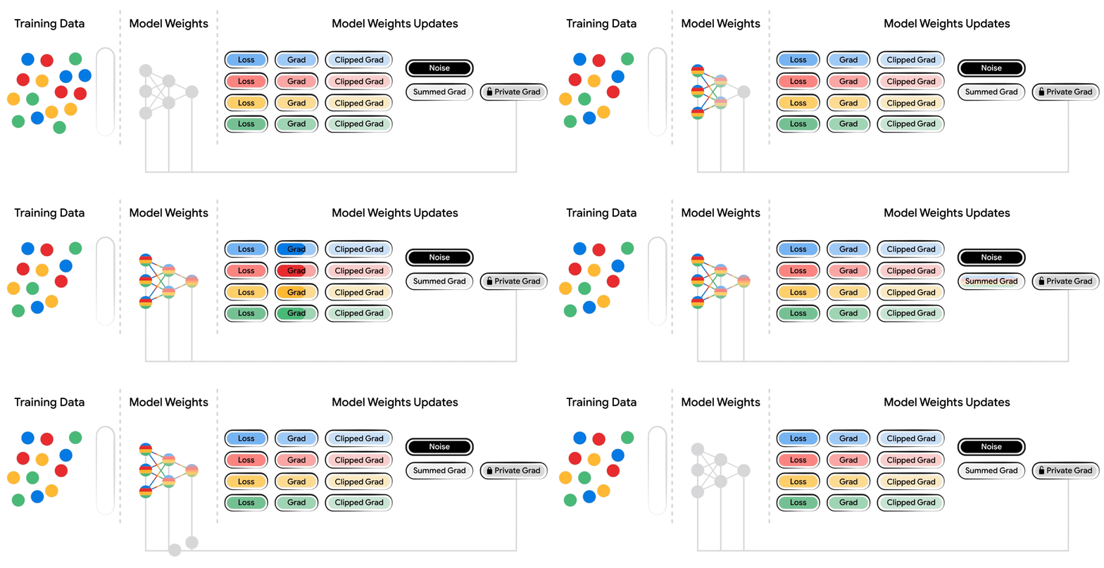
DP-SGD builds off of the stochastic gradient descent (SGD) optimizer with two modifications: (1) per-example gradients are clipped to a certain norm to limit sensitivity (the influence of an individual example on the overall model), which is a slow and computationally intensive process, and (2) a noisy gradient update is formed by taking aggregated gradients and adding noise that is proportional to the sensitivity and the strength of privacy guarantees.

DP-SGD is a modification of SGD that involves a) clipping per-example gradients to limit the sensitivity and b) adding the noise, calibrated to the sensitivity and privacy guarantees, to the aggregated gradients, before the gradient update step.


Existing DP-training challenges

Gradient noise injection methods usually exhibit: (1) loss of utility, (2) slower training, and (3) an increased memory footprint.

Loss of utility:

The best method for reducing utility drop is to use more computation. Using larger batch sizes and/or more iterations is one of the most prominent and practical ways of improving a model’s performance. Hyperparameter tuning is also extremely important but often overlooked. The utility of DP-trained models is sensitive to the total amount of noise added, which depends on hyperparameters, like the clipping norm and batch size. Additionally, other hyperparameters like the learning rate should be re-tuned to account for noisy gradient updates.

Another option is to obtain more data or use public data of similar distribution. This can be done by leveraging publicly available checkpoints, like ResNet or T5, and fine-tuning them using private data.

Slower training:

Most gradient noise injection methods limit sensitivity via clipping per-example gradients, considerably slowing down backpropagation. This can be addressed by choosing an efficient DP framework that efficiently implements per-example clipping.

Increased memory footprint:

DP-training requires significant memory for computing and storing per-example gradients. Additionally, it requires significantly larger batches to obtain better utility. Increasing the computation resources (e.g., the number and size of accelerators) is the simplest solution for extra memory requirements. Alternatively, several works advocate for gradient accumulation where smaller batches are combined to simulate a larger batch before the gradient update is applied. Further, some algorithms (e.g., ghost clipping, which is based on this paper) avoid per-example gradient clipping altogether.


Best practices

The following best practices can attain rigorous DP guarantees with the best model utility possible.

Choosing the right privacy unit:

First, we should be clear about a model’s privacy guarantees. This is encoded by selecting the “privacy unit,” which represents the neighboring dataset concept (i.e., datasets where only one row is different). Example-level protection is a common choice in the research literature, but may not be ideal, however, for user-generated data if individual users contributed multiple records to the training dataset. For such a case, user-level protection might be more appropriate. For text and sequence data, the choice of the unit is harder since in most applications individual training examples are not aligned to the semantic meaning embedded in the text.

Choosing privacy guarantees:

We outline three broad tiers of privacy guarantees and encourage practitioners to choose the lowest possible tier below:

  • Tier 1 — Strong privacy guarantees: Choosing ε ≤ 1 provides a strong privacy guarantee, but frequently results in a significant utility drop for large models and thus may only be feasible for smaller models.
  • Tier 2 — Reasonable privacy guarantees: We advocate for the currently undocumented, but still widely used, goal for DP-ML models to achieve an ε ≤ 10.
  • Tier 3 — Weak privacy guarantees: Any finite ε is an improvement over a model with no formal privacy guarantee. However, for ε > 10, the DP guarantee alone cannot be taken as sufficient evidence of data anonymization, and additional measures (e.g., empirical privacy auditing) may be necessary to ensure the model protects user data.

Hyperparameter tuning:

Choosing hyperparameters requires optimizing over three inter-dependent objectives: 1) model utility, 2) privacy cost ε, and 3) computation cost. Common strategies take two of the three as constraints, and focus on optimizing the third. We provide methods that will maximize the utility with a limited number of trials, e.g., tuning with privacy and computation constraints.

Reporting privacy guarantees:

A lot of works on DP for ML report only ε and possibly δ values for their training procedure. However, we believe that practitioners should provide a comprehensive overview of model guarantees that includes:

  1. DP setting: Are the results assuming central DP with a trusted service provider, local DP, or some other setting?
  2. Instantiating the DP definition:
    1. Data accesses covered: Whether the DP guarantee applies (only) to a single training run or also covers hyperparameter tuning etc.
    2. Final mechanism’s output: What is covered by the privacy guarantees and can be released publicly (e.g., model checkpoints, the full sequence of privatized gradients, etc.)
    3. Unit of privacy: The selected “privacy unit” (example-level, user-level, etc.)
    4. Adjacency definition for DP “neighboring” datasets: A description of how neighboring datasets differ (e.g., add-or-remove, replace-one, zero-out-one).
  3. Privacy accounting details: Providing accounting details, e.g., composition and amplification, are important for proper comparison between methods and should include:
    1. Type of accounting used, e.g., Rényi DP-based accounting, PLD accounting, etc.
    2. Accounting assumptions and whether they hold (e.g., Poisson sampling was assumed for privacy amplification but data shuffling was used in training).
    3. Formal DP statement for the model and tuning process (e.g., the specific ε, δ-DP or ρ-zCDP values).
  4. Transparency and verifiability: When possible, complete open-source code using standard DP libraries for the key mechanism implementation and accounting components.

Paying attention to all the components used:

Usually, DP-training is a straightforward application of DP-SGD or other algorithms. However, some components or losses that are often used in ML models (e.g., contrastive losses, graph neural network layers) should be examined to ensure privacy guarantees are not violated.


Open questions

While DP-ML is an active research area, we highlight the broad areas where there is room for improvement.

Developing better accounting methods:

Our current understanding of DP-training ε, δ guarantees relies on a number of techniques, like Rényi DP composition and privacy amplification. We believe that better accounting methods for existing algorithms will demonstrate that DP guarantees for ML models are actually better than expected.

Developing better algorithms:

The computational burden of using gradient noise injection for DP-training comes from the need to use larger batches and limit per-example sensitivity. Developing methods that can use smaller batches or identifying other ways (apart from per-example clipping) to limit the sensitivity would be a breakthrough for DP-ML.

Better optimization techniques:

Directly applying the same DP-SGD recipe is believed to be suboptimal for adaptive optimizers because the noise added to privatize the gradient may accumulate in learning rate computation. Designing theoretically grounded DP adaptive optimizers remains an active research topic. Another potential direction is to better understand the surface of DP loss, since for standard (non-DP) ML models flatter regions have been shown to generalize better.

Identifying architectures that are more robust to noise:

There's an opportunity to better understand whether we need to adjust the architecture of an existing model when introducing DP.


Conclusion

Our survey paper summarizes the current research related to making ML models DP, and provides practical tips on how to achieve the best privacy-utility trade offs. Our hope is that this work will serve as a reference point for the practitioners who want to effectively apply DP to complex ML models.


Acknowledgements

We thank Hussein Hazimeh, Zheng Xu , Carson Denison , H. Brendan McMahan, Sergei Vassilvitskii, Steve Chien and Abhradeep Thakurta, Badih Ghazi, Chiyuan Zhang for the help preparing this blog post, paper and tutorials content. Thanks to John Guilyard for creating the graphics in this post, and Ravi Kumar for comments.
Source: Google AI Blog


An ML-based approach to better characterize lung diseases

The combination of the environment an individual experiences and their genetic predispositions determines the majority of their risk for various diseases. Large national efforts, such as the UK Biobank, have created large, public resources to better understand the links between environment, genetics, and disease. This has the potential to help individuals better understand how to stay healthy, clinicians to treat illnesses, and scientists to develop new medicines.

One challenge in this process is how we make sense of the vast amount of clinical measurements — the UK Biobank has many petabytes of imaging, metabolic tests, and medical records spanning 500,000 individuals. To best use this data, we need to be able to represent the information present as succinct, informative labels about meaningful diseases and traits, a process called phenotyping. That is where we can use the ability of ML models to pick up on subtle intricate patterns in large amounts of data.

We’ve previously demonstrated the ability to use ML models to quickly phenotype at scale for retinal diseases. Nonetheless, these models were trained using labels from clinician judgment, and access to clinical-grade labels is a limiting factor due to the time and expense needed to create them.

In “Inference of chronic obstructive pulmonary disease with deep learning on raw spirograms identifies new genetic loci and improves risk models”, published in Nature Genetics, we’re excited to highlight a method for training accurate ML models for genetic discovery of diseases, even when using noisy and unreliable labels. We demonstrate the ability to train ML models that can phenotype directly from raw clinical measurement and unreliable medical record information. This reduced reliance on medical domain experts for labeling greatly expands the range of applications for our technique to a panoply of diseases and has the potential to improve their prevention, diagnosis, and treatment. We showcase this method with ML models that can better characterize lung function and chronic obstructive pulmonary disease (COPD). Additionally, we show the usefulness of these models by demonstrating a better ability to identify genetic variants associated with COPD, improved understanding of the biology behind the disease, and successful prediction of outcomes associated with COPD.


ML for deeper understanding of exhalation

For this demonstration, we focused on COPD, the third leading cause of worldwide death in 2019, in which airway inflammation and impeded airflow can progressively reduce lung function. Lung function for COPD and other diseases is measured by recording an individual’s exhalation volume over time (the record is called a spirogram; see an example below). Although there are guidelines (called GOLD) for determining COPD status from exhalation, these use only a few, specific data points in the curve and apply fixed thresholds to those values. Much of the rich data from these spirograms is discarded in this analysis of lung function.

We reasoned that ML models trained to classify spirograms would be able to use the rich data present more completely and result in more accurate and comprehensive measures of lung function and disease, similar to what we have seen in other classification tasks like mammography or histology. We trained ML models to predict whether an individual has COPD using the full spirograms as inputs.

Spirometry and COPD status overview. Spirograms from lung function test showing a forced expiratory volume-time spirogram (left), a forced expiratory flow-time spirogram (middle), and an interpolated forced expiratory flow-volume spirogram (right). The profile of individuals w/o COPD is different.

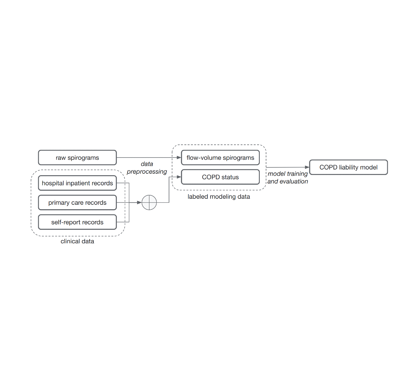
The common method of training models for this problem, supervised learning, requires samples to be associated with labels. Determining those labels can require the effort of very time-constrained experts. For this work, to show that we do not necessarily need medically graded labels, we decided to use a variety of widely available sources of medical record information to create those labels without medical expert review. These labels are less reliable and noisy for two reasons. First, there are gaps in the medical records of individuals because they use multiple health services. Second, COPD is often undiagnosed, meaning many with the disease will not be labeled as having it even if we compile the complete medical records. Nonetheless, we trained a model to predict these noisy labels from the spirogram curves and treat the model predictions as a quantitative COPD liability or risk score.

Noisy COPD status labels were derived using various medical record sources (clinical data). A COPD liability model is then trained to predict COPD status from raw flow-volume spirograms.

Predicting COPD outcomes

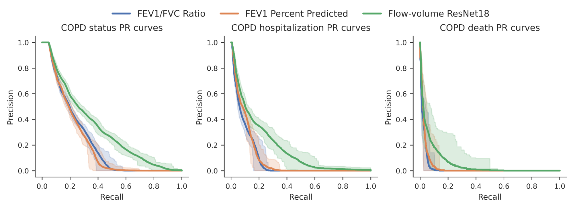
We then investigated whether the risk scores produced by our model could better predict a variety of binary COPD outcomes (for example, an individual’s COPD status, whether they were hospitalized for COPD or died from it). For comparison, we benchmarked the model relative to expert-defined measurements required to diagnose COPD, specifically FEV1/FVC, which compares specific points on the spirogram curve with a simple mathematical ratio. We observed an improvement in the ability to predict these outcomes as seen in the precision-recall curves below.

Precision-recall curves for COPD status and outcomes for our ML model (green) compared to traditional measures. Confidence intervals are shown by lighter shading.

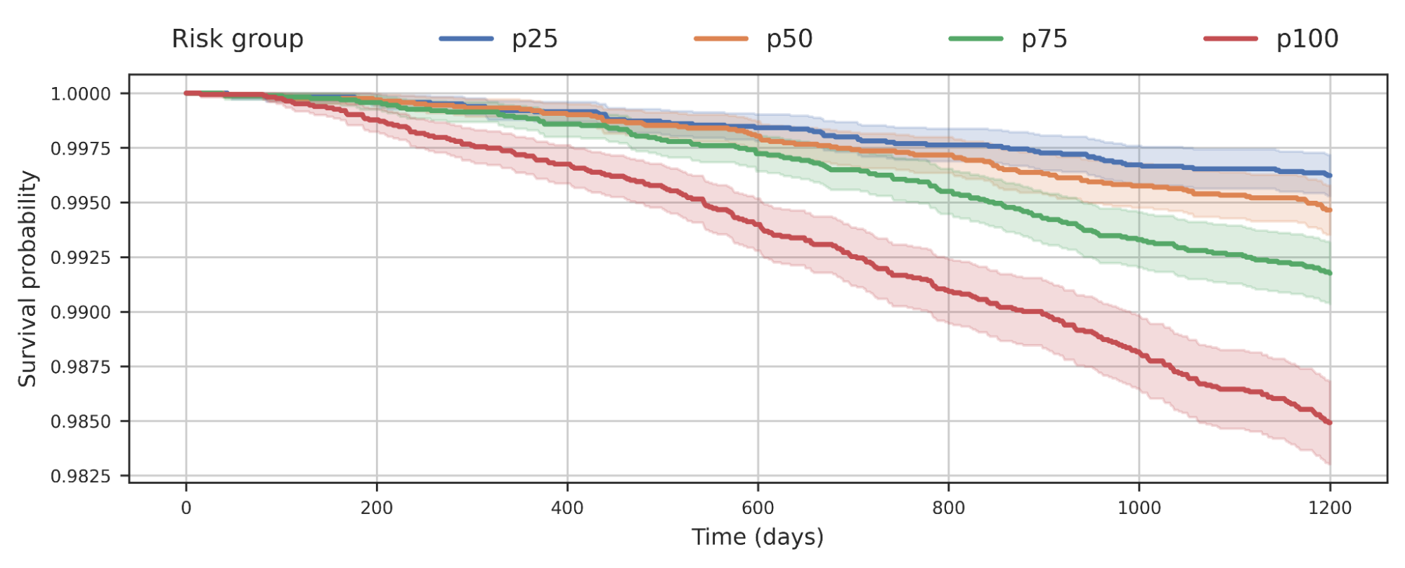
We also observed that separating populations by their COPD model score was predictive of all-cause mortality. This plot suggests that individuals with higher COPD risk are more likely to die earlier from any causes and the risk probably has implications beyond just COPD.

Survival analysis of a cohort of UK Biobank individuals stratified by their COPD model’s predicted risk quartile. The decrease of the curve indicates individuals in the cohort dying over time. For example, p100 represents the 25% of the cohort with greatest predicted risk, while p50 represents the 2nd quartile.

Identifying the genetic links with COPD

Since the goal of large scale biobanks is to bring together large amounts of both phenotype and genetic data, we also performed a test called a genome-wide association study (GWAS) to identify the genetic links with COPD and genetic predisposition. A GWAS measures the strength of the statistical association between a given genetic variant — a change in a specific position of DNA — and the observations (e.g., COPD) across a cohort of cases and controls. Genetic associations discovered in this manner can inform drug development that modifies the activity or products of a gene, as well as expand our understanding of the biology for a disease.

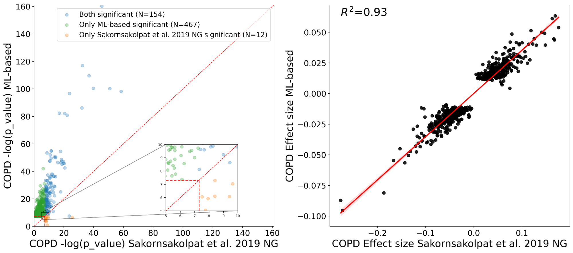
We showed with our ML-phenotyping method that not only do we rediscover almost all known COPD variants found by manual phenotyping, but we also find many novel genetic variants significantly associated with COPD. In addition, we see good agreement on the effect sizes for the variants discovered by both our ML approach and the manual one (R2=0.93), which provides strong evidence for validity of the newly found variants.

Left: A plot comparing the statistical power of genetic discovery using the labels for our ML model (y-axis) with the statistical power of the manual labels from a traditional study (x-axis). A value above the y = x line indicates greater statistical power in our method. Green points indicate significant findings in our method that are not found using the traditional approach. Orange points are significant in the traditional approach but not ours. Blue points are significant in both. Right: Estimates of the association effect between our method (y-axis) and traditional method (x-axis). Note that the relative values between studies are comparable but the absolute numbers are not.

Finally, our collaborators at Harvard Medical School and Brigham and Women’s Hospital further examined the plausibility of these findings by providing insights into the possible biological role of the novel variants in development and progression of COPD (you can see more discussion on these insights in the paper).


Conclusion

We demonstrated that our earlier methods for phenotyping with ML can be expanded to a wide range of diseases and can provide novel and valuable insights. We made two key observations by using this to predict COPD from spirograms and discovering new genetic insights. First, domain knowledge was not necessary to make predictions from raw medical data. Interestingly, we showed the raw medical data is probably underutilized and the ML model can find patterns in it that are not captured by expert-defined measurements. Second, we do not need medically graded labels; instead, noisy labels defined from widely available medical records can be used to generate clinically predictive and genetically informative risk scores. We hope that this work will broadly expand the ability of the field to use noisy labels and will improve our collective understanding of lung function and disease.


Acknowledgments

This work is the combined output of multiple contributors and institutions. We thank all contributors: Justin Cosentino, Babak Alipanahi, Zachary R. McCaw, Cory Y. McLean, Farhad Hormozdiari (Google), Davin Hill (Northeastern University), Tae-Hwi Schwantes-An and Dongbing Lai (Indiana University), Brian D. Hobbs and Michael H. Cho (Brigham and Women’s Hospital, and Harvard Medical School). We also thank Ted Yun and Nick Furlotte for reviewing the manuscript, Greg Corrado and Shravya Shetty for support, and Howard Yang, Kavita Kulkarni, and Tammi Huynh for helping with publication logistics.

Source: Google AI Blog


Visual Blocks for ML: Accelerating machine learning prototyping with interactive tools

Recent deep learning advances have enabled a plethora of high-performance, real-time multimedia applications based on machine learning (ML), such as human body segmentation for video and teleconferencing, depth estimation for 3D reconstruction, hand and body tracking for interaction, and audio processing for remote communication.

However, developing and iterating on these ML-based multimedia prototypes can be challenging and costly. It usually involves a cross-functional team of ML practitioners who fine-tune the models, evaluate robustness, characterize strengths and weaknesses, inspect performance in the end-use context, and develop the applications. Moreover, models are frequently updated and require repeated integration efforts before evaluation can occur, which makes the workflow ill-suited to design and experiment.

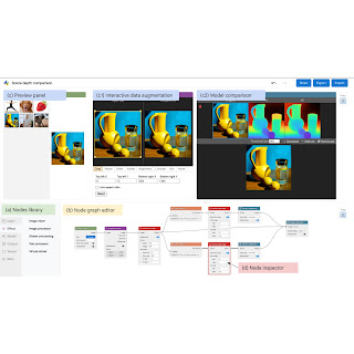
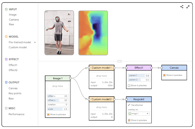
In “Rapsai: Accelerating Machine Learning Prototyping of Multimedia Applications through Visual Programming”, presented at CHI 2023, we describe a visual programming platform for rapid and iterative development of end-to-end ML-based multimedia applications. Visual Blocks for ML, formerly called Rapsai, provides a no-code graph building experience through its node-graph editor. Users can create and connect different components (nodes) to rapidly build an ML pipeline, and see the results in real-time without writing any code. We demonstrate how this platform enables a better model evaluation experience through interactive characterization and visualization of ML model performance and interactive data augmentation and comparison. Sign up to be notified when Visual Blocks for ML is publicly available.

Visual Blocks uses a node-graph editor that facilitates rapid prototyping of ML-based multimedia applications.


Formative study: Design goals for rapid ML prototyping

To better understand the challenges of existing rapid prototyping ML solutions (LIME, VAC-CNN, EnsembleMatrix), we conducted a formative study (i.e., the process of gathering feedback from potential users early in the design process of a technology product or system) using a conceptual mock-up interface. Study participants included seven computer vision researchers, audio ML researchers, and engineers across three ML teams.

The formative study used a conceptual mock-up interface to gather early insights.

Through this formative study, we identified six challenges commonly found in existing prototyping solutions:

  1. The input used to evaluate models typically differs from in-the-wild input with actual users in terms of resolution, aspect ratio, or sampling rate.
  2. Participants could not quickly and interactively alter the input data or tune the model.
  3. Researchers optimize the model with quantitative metrics on a fixed set of data, but real-world performance requires human reviewers to evaluate in the application context.
  4. It is difficult to compare versions of the model, and cumbersome to share the best version with other team members to try it.
  5. Once the model is selected, it can be time-consuming for a team to make a bespoke prototype that showcases the model.
  6. Ultimately, the model is just part of a larger real-time pipeline, in which participants desire to examine intermediate results to understand the bottleneck.

These identified challenges informed the development of the Visual Blocks system, which included six design goals: (1) develop a visual programming platform for rapidly building ML prototypes, (2) support real-time multimedia user input in-the-wild, (3) provide interactive data augmentation, (4) compare model outputs with side-by-side results, (5) share visualizations with minimum effort, and (6) provide off-the-shelf models and datasets.


Node-graph editor for visually programming ML pipelines

Visual Blocks is mainly written in JavaScript and leverages TensorFlow.js and TensorFlow Lite for ML capabilities and three.js for graphics rendering. The interface enables users to rapidly build and interact with ML models using three coordinated views: (1) a Nodes Library that contains over 30 nodes (e.g., Image Processing, Body Segmentation, Image Comparison) and a search bar for filtering, (2) a Node-graph Editor that allows users to build and adjust a multimedia pipeline by dragging and adding nodes from the Nodes Library, and (3) a Preview Panel that visualizes the pipeline’s input and output, alters the input and intermediate results, and visually compares different models.

The visual programming interface allows users to quickly develop and evaluate ML models by composing and previewing node-graphs with real-time results.


Iterative design, development, and evaluation of unique rapid prototyping capabilities

Over the last year, we’ve been iteratively designing and improving the Visual Blocks platform. Weekly feedback sessions with the three ML teams from the formative study showed appreciation for the platform’s unique capabilities and its potential to accelerate ML prototyping through:

  • Support for various types of input data (image, video, audio) and output modalities (graphics, sound).
  • A library of pre-trained ML models for common tasks (body segmentation, landmark detection, portrait depth estimation) and custom model import options.
  • Interactive data augmentation and manipulation with drag-and-drop operations and parameter sliders.
  • Side-by-side comparison of multiple models and inspection of their outputs at different stages of the pipeline.
  • Quick publishing and sharing of multimedia pipelines directly to the web.

Evaluation: Four case studies

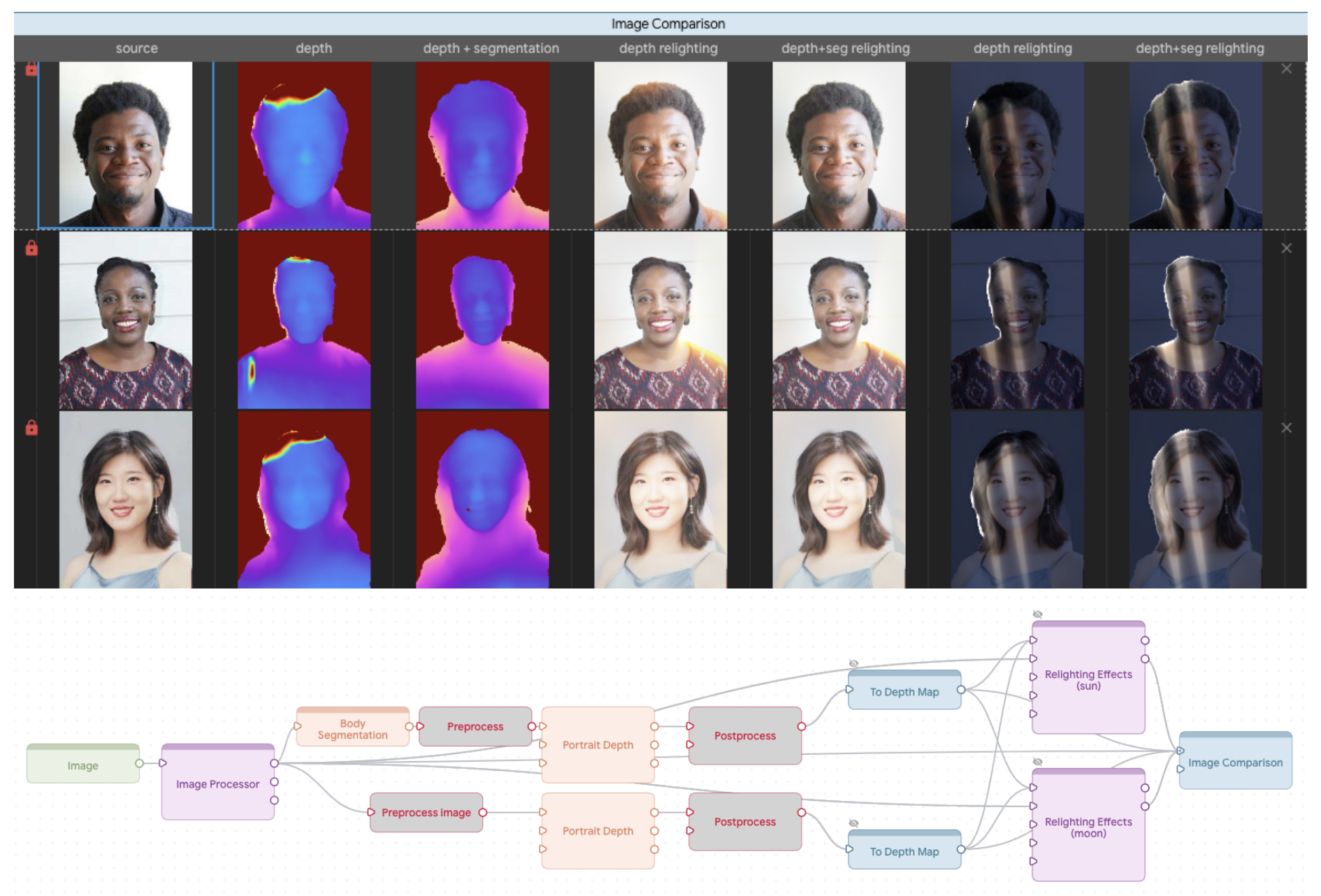
To evaluate the usability and effectiveness of Visual Blocks, we conducted four case studies with 15 ML practitioners. They used the platform to prototype different multimedia applications: portrait depth with relighting effects, scene depth with visual effects, alpha matting for virtual conferences, and audio denoising for communication.

The system streamlining comparison of two Portrait Depth models, including customized visualization and effects.

With a short introduction and video tutorial, participants were able to quickly identify differences between the models and select a better model for their use case. We found that Visual Blocks helped facilitate rapid and deeper understanding of model benefits and trade-offs:

“It gives me intuition about which data augmentation operations that my model is more sensitive [to], then I can go back to my training pipeline, maybe increase the amount of data augmentation for those specific steps that are making my model more sensitive.” (Participant 13)
“It’s a fair amount of work to add some background noise, I have a script, but then every time I have to find that script and modify it. I’ve always done this in a one-off way. It’s simple but also very time consuming. This is very convenient.” (Participant 15)
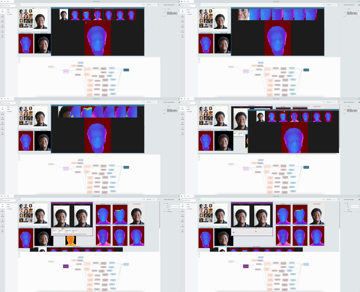
The system allows researchers to compare multiple Portrait Depth models at different noise levels, helping ML practitioners identify the strengths and weaknesses of each.

In a post-hoc survey using a seven-point Likert scale, participants reported Visual Blocks to be more transparent about how it arrives at its final results than Colab (Visual Blocks 6.13 ± 0.88 vs. Colab 5.0 ± 0.88, 𝑝 < .005) and more collaborative with users to come up with the outputs (Visual Blocks 5.73 ± 1.23 vs. Colab 4.15 ± 1.43, 𝑝 < .005). Although Colab assisted users in thinking through the task and controlling the pipeline more effectively through programming, Users reported that they were able to complete tasks in Visual Blocks in just a few minutes that could normally take up to an hour or more. For example, after watching a 4-minute tutorial video, all participants were able to build a custom pipeline in Visual Blocks from scratch within 15 minutes (10.72 ± 2.14). Participants usually spent less than five minutes (3.98 ± 1.95) getting the initial results, then were trying out different input and output for the pipeline.

User ratings between Rapsai (initial prototype of Visual Blocks) and Colab across five dimensions.

More results in our paper showed that Visual Blocks helped participants accelerate their workflow, make more informed decisions about model selection and tuning, analyze strengths and weaknesses of different models, and holistically evaluate model behavior with real-world input.


Conclusions and future directions

Visual Blocks lowers development barriers for ML-based multimedia applications. It empowers users to experiment without worrying about coding or technical details. It also facilitates collaboration between designers and developers by providing a common language for describing ML pipelines. In the future, we plan to open this framework up for the community to contribute their own nodes and integrate it into many different platforms. We expect visual programming for machine learning to be a common interface across ML tooling going forward.


Acknowledgements

This work is a collaboration across multiple teams at Google. Key contributors to the project include Ruofei Du, Na Li, Jing Jin, Michelle Carney, Xiuxiu Yuan, Kristen Wright, Mark Sherwood, Jason Mayes, Lin Chen, Jun Jiang, Scott Miles, Maria Kleiner, Yinda Zhang, Anuva Kulkarni, Xingyu "Bruce" Liu, Ahmed Sabie, Sergio Escolano, Abhishek Kar, Ping Yu, Ram Iyengar, Adarsh Kowdle, and Alex Olwal.

We would like to extend our thanks to Jun Zhang and Satya Amarapalli for a few early-stage prototypes, and Sarah Heimlich for serving as a 20% program manager, Sean Fanello, Danhang Tang, Stephanie Debats, Walter Korman, Anne Menini, Joe Moran, Eric Turner, and Shahram Izadi for providing initial feedback for the manuscript and the blog post. We would also like to thank our CHI 2023 reviewers for their insightful feedback.

Source: Google AI Blog


Leveraging transfer learning for large scale differentially private image classification

Large deep learning models are becoming the workhorse of a variety of critical machine learning (ML) tasks. However, it has been shown that without any protection it is plausible for bad actors to attack a variety of models, across modalities, to reveal information from individual training examples. As such, it’s essential to protect against this sort of information leakage.

Differential privacy (DP) provides formal protection against an attacker who aims to extract information about the training data. The most popular method for DP training in deep learning is differentially private stochastic gradient descent (DP-SGD). The core recipe implements a common theme in DP: “fuzzing” an algorithm’s outputs with noise to obscure the contributions of any individual input.

In practice, DP training can be very expensive or even ineffective for very large models. Not only does the computational cost typically increase when requiring privacy guarantees, but the noise also increases proportionally. Given these challenges, there has recently been much interest in developing methods that enable efficient DP training. The goal is to develop simple and practical methods for producing high-quality large-scale private models.

The ImageNet classification benchmark is an effective test bed for this goal because 1) it is a challenging task even in the non-private setting, that requires sufficiently large models to successfully classify large numbers of varied images and 2) it is a public, open-source dataset, which other researchers can access and use for collaboration. With this approach, researchers may simulate a practical situation where a large model is required to train on private data with DP guarantees.

To that end, today we discuss improvements we’ve made in training high-utility, large-scale private models. First, in “Large-Scale Transfer Learning for Differentially Private Image Classification”, we share strong results on the challenging task of image classification on the ImageNet-1k dataset with DP constraints. We show that with a combination of large-scale transfer learning and carefully chosen hyperparameters it is indeed possible to significantly reduce the gap between private and non-private performance even on challenging tasks and high-dimensional models. Then in “Differentially Private Image Classification from Features”, we further show that privately fine-tuning just the last layer of pre-trained model with more advanced optimization algorithms improves the performance even further, leading to new state-of-the-art DP results across a variety of popular image classification benchmarks, including ImageNet-1k. To encourage further development in this direction and enable other researchers to verify our findings, we are also releasing the associated source code.


Transfer learning and differential privacy

The main idea behind transfer learning is to reuse the knowledge gained from solving one problem and then apply it to a related problem. This is especially useful when there is limited or low-quality data available for the target problem as it allows us to leverage the knowledge gained from a larger and more diverse public dataset.

In the context of DP, transfer learning has emerged as a promising technique to improve the accuracy of private models, by leveraging knowledge learned from pre-training tasks. For example, if a model has already been trained on a large public dataset for a similar privacy-sensitive task, it can be fine-tuned on a smaller and more specific dataset for the target DP task. More specifically, one first pre-trains a model on a large dataset with no privacy concerns, and then privately fine-tunes the model on the sensitive dataset. In our work, we improve the effectiveness of DP transfer learning and illustrate it by simulating private training on publicly available datasets, namely ImageNet-1k, CIFAR-100, and CIFAR-10.


Better pre-training improves DP performance

To start exploring how transfer learning can be effective for differentially private image classification tasks, we carefully examined hyperparameters affecting DP performance. Surprisingly, we found that with carefully chosen hyperparameters (e.g., initializing the last layer to zero and choosing large batch sizes), privately fine-tuning just the last layer of a pre-trained model yields significant improvements over the baseline. Training just the last layer also significantly improves the cost-utility ratio of training a high-quality image classification model with DP.

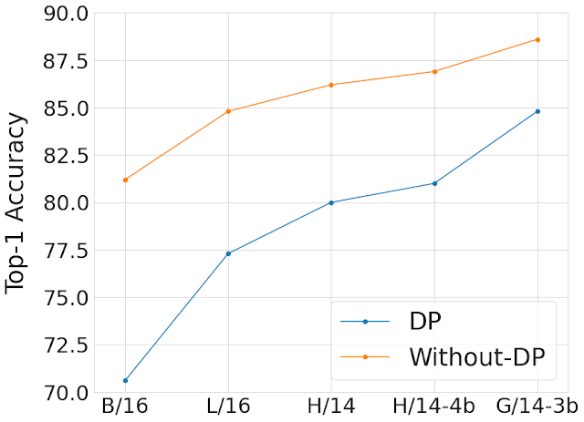
As shown below, we compare the performance on ImageNet of the best hyperparameter recommendations both with and without privacy and across a variety of model and pre-training dataset sizes. We find that scaling the model and using a larger pre-training dataset decreases the gap in accuracy coming from the addition of the privacy guarantee. Typically, privacy guarantees of a system are characterized by a positive parameter ε, with smaller ε corresponding to better privacy. In the following figure, we use the privacy guarantee of ε = 10.

Comparing our best models with and without privacy on ImageNet across model and pre-training dataset sizes. The X-axis shows the different Vision Transformer models we used for this study in ascending order of model size from left to right. We used JFT-300M to pretrain B/16, L/16 and H/14 models, JFT-4B (a larger version of JFT-3B) to pretrain H/14-4b and JFT-3B to pretrain G/14-3b. We do this in order to study the effectiveness of jointly scaling the model and pre-training dataset (JFT-3B or 4B). The Y-axis shows the Top-1 accuracy on ImageNet-1k test set once the model is finetuned (in the private or non-private way) with the ImageNet-1k training set. We consistently see that the scaling of the model and the pre-training dataset size decreases the gap in accuracy coming from the addition of the privacy guarantee of ε = 10.

Better optimizers improve DP performance

Somewhat surprisingly, we found that privately training just the last layer of a pre-trained model provides the best utility with DP. While past studies [1, 2, 3] largely relied on using first-order differentially private training algorithms like DP-SGD for training large models, in the specific case of privately learning just the last layer from features, we observe that computational burden is often low enough to allow for more sophisticated optimization schemes, including second-order methods (e.g., Newton or Quasi-Newton methods), which can be more accurate but also more computationally expensive.

In “Differentially Private Image Classification from Features”, we systematically explore the effect of loss functions and optimization algorithms. We find that while the commonly used logistic regression performs better than linear regression in the non-private setting, the situation is reversed in the private setting: least-squares linear regression is much more effective than logistic regression from both a privacy and computational standpoint for typical range of ε values ([1, 10]), and even more effective for stricter epsilon values (ε < 1).

We further explore using DP Newton’s method to solve logistic regression. We find that this is still outperformed by DP linear regression in the high privacy regime. Indeed, Newton's method involves computing a Hessian (a matrix that captures second-order information), and making this matrix differentially private requires adding far more noise in logistic regression than in linear regression, which has a highly structured Hessian.

Building on this observation, we introduce a method that we call differentially private SGD with feature covariance (DP-FC), where we simply replace the Hessian in logistic regression with privatized feature covariance. Since feature covariance only depends on the inputs (and neither on model parameters nor class labels), we are able to share it across classes and training iterations, thus greatly reducing the amount of noise that needs to be added to protect it. This allows us to combine the benefits of using logistic regression with the efficient privacy protection of linear regression, leading to improved privacy-utility trade-off.

With DP-FC, we surpass previous state-of-the-art results considerably on three private image classification benchmarks, namely ImageNet-1k, CIFAR-10 and CIFAR-100, just by performing DP fine-tuning on features extracted from a powerful pre-trained model.

Comparison of top-1 accuracies (Y-axis) with private fine-tuning using DP-FC method on all three datasets across a range of ε (X-axis). We observe that better pre-training helps even more for lower values of ε (stricter privacy guarantee).

Conclusion

We demonstrate that large-scale pre-training on a public dataset is an effective strategy for obtaining good results when fine-tuned privately. Moreover, scaling both model size and pre-training dataset improves performance of the private model and narrows the quality gap compared to the non-private model. We further provide strategies to effectively use transfer learning for DP. Note that this work has several limitations worth considering — most importantly our approach relies on the availability of a large and trustworthy public dataset, which can be challenging to source and vet. We hope that our work is useful for training large models with meaningful privacy guarantees!


Acknowledgements

In addition to the authors of this blogpost, this research was conducted by Abhradeep Thakurta, Alex Kurakin and Ashok Cutkosky. We are also grateful to the developers of Jax, Flax, and Scenic libraries. Specifically, we would like to thank Mostafa Dehghani for helping us with Scenic and high-performance vision baselines and Lucas Beyer for help with deduping the JFT data. We are also grateful to Li Zhang, Emil Praun, Andreas Terzis, Shuang Song, Pierre Tholoniat, Roxana Geambasu, and Steve Chien for stimulating discussions on differential privacy throughout the project. Additionally, we thank anonymous reviewers, Gautam Kamath and Varun Kanade for helpful feedback throughout the publication process. Finally, we would like to thank John Anderson and Corinna Cortes from Google Research, Borja Balle, Soham De, Sam Smith, Leonard Berrada, and Jamie Hayes from DeepMind for generous feedback.

Source: Google AI Blog


Teaching old labels new tricks in heterogeneous graphs

Industrial applications of machine learning are commonly composed of various items that have differing data modalities or feature distributions. Heterogeneous graphs (HGs) offer a unified view of these multimodal data systems by defining multiple types of nodes (for each data type) and edges (for the relation between data items). For instance, e-commerce networks might have [user, product, review] nodes or video platforms might have [channel, user, video, comment] nodes. Heterogeneous graph neural networks (HGNNs) learn node embeddings summarizing each node’s relationships into a vector. However, in real world HGs, there is often a label imbalance issue between different node types. This means that label-scarce node types cannot exploit HGNNs, which hampers the broader applicability of HGNNs.

In “Zero-shot Transfer Learning within a Heterogeneous Graph via Knowledge Transfer Networks”, presented at NeurIPS 2022, we propose a model called a Knowledge Transfer Network (KTN), which transfers knowledge from label-abundant node types to zero-labeled node types using the rich relational information given in a HG. We describe how we pre-train a HGNN model without the need for fine-tuning. KTNs outperform state-of-the-art transfer learning baselines by up to 140% on zero-shot learning tasks, and can be used to improve many existing HGNN models on these tasks by 24% (or more).

KTNs transform labels from one type of information (squares) through a graph to another type (stars).


What is a heterogeneous graph?

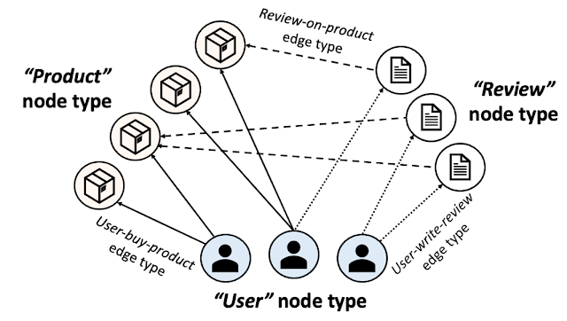
A HG is composed of multiple node and edge types. The figure below shows an e-commerce network presented as a HG. In e-commerce, “users” purchase “products” and write “reviews”. A HG presents this ecosystem using three node types [user, product, review] and three edge types [user-buy-product, user-write-review, review-on-product]. Individual products, users, and reviews are then presented as nodes and their relationships as edges in the HG with the corresponding node and edge types.

E-commerce heterogeneous graph.

In addition to all connectivity information, HGs are commonly given with input node attributes that summarize each node’s information. Input node attributes could have different modalities across different node types. For instance, images of products could be given as input node attributes for the product nodes, while text can be given as input attributes to review nodes. Node labels (e.g., the category of each product or the category that most interests each user) are what we want to predict on each node.


HGNNs and label scarcity issues

HGNNs compute node embeddings that summarize each node’s local structures (including the node and its neighbor’s information). These node embeddings are utilized by a classifier to predict each node’s label. To train a HGNN model and a classifier to predict labels for a specific node type, we require a good amount of labels for the type.

A common issue in industrial applications of deep learning is label scarcity, and with their diverse node types, HGNNs are even more likely to face this challenge. For instance, publicly available content node types (e.g., product nodes) are abundantly labeled, whereas labels for user or account nodes may not be available due to privacy restrictions. This means that in most standard training settings, HGNN models can only learn to make good inferences for a few label-abundant node types and can usually not make any inferences for any remaining node types (given the absence of any labels for them).


Transfer learning on heterogeneous graphs

Zero-shot transfer learning is a technique used to improve the performance of a model on a target domain with no labels by using the knowledge learned by the model from another related source domain with adequately labeled data. To apply transfer learning to solve this label scarcity issue for certain node types in HGs, the target domain would be the zero-labeled node types. Then what would be the source domain? Previous work commonly sets the source domain as the same type of nodes located in a different HG, assuming those nodes are abundantly labeled. This graph-to-graph transfer learning approach pre-trains a HGNN model on the external HG and then runs the model on the original (label-scarce) HG.

However, these approaches are not applicable in many real-world scenarios for three reasons. First, any external HG that could be used in a graph-to-graph transfer learning setting would almost surely be proprietary, thus, likely unavailable. Second, even if practitioners could obtain access to an external HG, it is unlikely the distribution of that source HG would match their target HG well enough to apply transfer learning. Finally, node types suffering from label scarcity are likely to suffer the same issue on other HGs (e.g., privacy issues on user nodes).


Our approach: Transfer learning between node types within a heterogeneous graph

Here, we shed light on a more practical source domain, other node types with abundant labels located on the same HG. Instead of using extra HGs, we transfer knowledge within a single HG (assumed to be fully owned by the practitioners) across different types of nodes. More specifically, we pre-train a HGNN model and a classifier on a label-abundant (source) node type, then reuse the models on the zero-labeled (target) node types located in the same HG without additional fine-tuning. The one requirement is that the source and target node types share the same label set (e.g., in the e-commerce HG, product nodes have a label set describing product categories, and user nodes share the same label set describing their favorite shopping categories).


Why is it challenging?

Unfortunately, we cannot directly reuse the pre-trained HGNN and classifier on the target node type. One crucial characteristic of HGNN architectures is that they are composed of modules specialized to each node type to fully learn the multiplicity of HGs. HGNNs use distinct sets of modules to compute embeddings for each node type. In the figure below, blue- and red-colored modules are used to compute node embeddings for the source and target node types, respectively.

HGNNs are composed of modules specialized to each node type and use distinct sets of modules to compute embeddings of different node types. More details can be found in the paper.

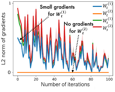
While pre-training HGNNs on the source node type, source-specific modules in the HGNNs are well trained, however target-specific modules are under-trained as they have only a small amount of gradients flowing into them. This is shown below, where we see that the L2 norm of gradients for target node types (i.e., Mtt) are much lower than for source types (i.e., Mss). In this case a HGNN model outputs poor node embeddings for the target node type, which results in poor task performance.

In HGNNs, target type-specific modules receive zero or only a small amount of gradients during pre-training on the source node type, leading to poor performance on the target node type.

KTN: Trainable cross-type transfer learning for HGNNs

Our work focuses on transforming the (poor) target node embeddings computed by a pre-trained HGNN model to follow the distribution of the source node embeddings. Then the classifier, pre-trained on the source node type, can be reused for the target node type. How can we map the target node embeddings to the source domain? To answer this question, we investigate how HGNNs compute node embeddings to learn the relationship between source and target distributions.

HGNNs aggregate connected node embeddings to augment a target node’s embeddings in each layer. In other words, the node embeddings for both source and target node types are updated using the same input — the previous layer’s node embeddings of any connected node types. This means that they can be represented by each other. We prove this relationship theoretically and find there is a mapping matrix (defined by HGNN parameters) from the target domain to the source domain (more details in Theorem 1 in the paper). Based on this theorem, we introduce an auxiliary neural network, which we refer to as a Knowledge Transfer Network (KTN), that receives the target node embeddings and then transforms them by multiplying them with a (trainable) mapping matrix. We then define a regularizer that is minimized along with the performance loss in the pre-training phase to train the KTN. At test time, we map the target embeddings computed from the pre-trained HGNN to the source domain using the trained KTN for classification.

In HGNNs, the final node embeddings of both source and target types are computed from different mathematical functions (f(): source, g(): target) which use the same input — the previous layer’s node embeddings.

Experimental results

To examine the effectiveness of KTNs, we ran 18 different zero-shot transfer learning tasks on two public heterogeneous graphs, Open Academic Graph and Pubmed. We compare KTN with eight state-of-the-art transfer learning methods (DAN, JAN, DANN, CDAN, CDAN-E, WDGRL, LP, EP). Shown below, KTN consistently outperforms all baselines on all tasks, beating transfer learning baselines by up to 140% (as measured by Normalized Discounted Cumulative Gain, a ranking metric).

Zero-shot transfer learning on Open Academic Graph (OAG-CS) and Pubmed datasets. The colors represent different categories of transfer learning baselines against which the results are compared. Yellow: Use statistical properties (e.g., mean, variance) of distributions. Green: Use adversarial models to transfer knowledge. Orange: Transfer knowledge directly via graph structure using label propagation.

Most importantly, KTN can be applied to almost all HGNN models that have node and edge type-specific parameters and improve their zero-shot performance on target domains. As shown below, KTN improves accuracy on zero-labeled node types across six different HGNN models(R-GCN, HAN, HGT, MAGNN, MPNN, H-MPNN) by up to 190%.

KTN can be applied to six different HGNN models and improve their zero-shot performance on target domains.

Takeaways

Various ecosystems in industry can be presented as heterogeneous graphs. HGNNs summarize heterogeneous graph information into effective representations. However, label scarcity issues on certain types of nodes prevent the wider application of HGNNs. In this post, we introduced KTN, the first cross-type transfer learning method designed for HGNNs. With KTN, we can fully exploit the richness of heterogeneous graphs via HGNNs regardless of label scarcity. See the paper for more details.


Acknowledgements

This paper is joint work with our co-authors John Palowitch (Google Research), Dustin Zelle (Google Research), Ziniu Hu (Intern, Google Research), and Russ Salakhutdinov (CMU). We thank Tom Small for creating the animated figure in this blog post.

Source: Google AI Blog


Accelerating Text Generation with Confident Adaptive Language Modeling (CALM)

Language models (LMs) are the driving force behind many recent breakthroughs in natural language processing. Models like T5, LaMDA, GPT-3, and PaLM have demonstrated impressive performance on various language tasks. While multiple factors can contribute to improving the performance of LMs, some recent studies suggest that scaling up the model’s size is crucial for revealing emergent capabilities. In other words, some instances can be solved by small models, while others seem to benefit from increased scale.

Despite recent efforts that enabled the efficient training of LMs over large amounts of data, trained models can still be slow and costly for practical use. When generating text at inference time, most autoregressive LMs output content similar to how we speak and write (word after word), predicting each new word based on the preceding words. This process cannot be parallelized since LMs need to complete the prediction of one word before starting to compute the next one. Moreover, predicting each word requires significant computation given the model’s billions of parameters.

In “Confident Adaptive Language Modeling”, presented at NeurIPS 2022, we introduce a new method for accelerating the text generation of LMs by improving efficiency at inference time. Our method, named CALM, is motivated by the intuition that some next word predictions are easier than others. When writing a sentence, some continuations are trivial, while others might require more effort. Current LMs devote the same amount of compute power for all predictions. Instead, CALM dynamically distributes the computational effort across generation timesteps. By selectively allocating more computational resources only to harder predictions, CALM generates text faster while preserving output quality.


Confident Adaptive Language Modeling

When possible, CALM skips some compute effort for certain predictions. To demonstrate this, we use the popular encoder-decoder T5 architecture. The encoder reads the input text (e.g., a news article to summarize) and converts the text to dense representations. Then, the decoder outputs the summary by predicting it word by word. Both the encoder and decoder include a long sequence of Transformer layers. Each layer includes attention and feedforward modules with many matrix multiplications. These layers gradually modify the hidden representation that is ultimately used for predicting the next word.

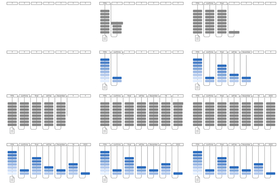
Instead of waiting for all decoder layers to complete, CALM attempts to predict the next word earlier, after some intermediate layer. To decide whether to commit to a certain prediction or to postpone the prediction to a later layer, we measure the model’s confidence in its intermediate prediction. The rest of the computation is skipped only when the model is confident enough that the prediction won’t change. For quantifying what is “confident enough”, we calibrate a threshold that statistically satisfies arbitrary quality guarantees over the full output sequence.

Text generation with a regular language model (top) and with CALM (bottom). CALM attempts to make early predictions. Once confident enough (darker blue tones), it skips ahead and saves time.

Language Models with Early Exits

Enabling this early exit strategy for LMs requires minimal modifications to the training and inference processes. During training, we encourage the model to produce meaningful representations in intermediate layers. Instead of predicting only using the top layer, our learning loss function is a weighted average over the predictions of all layers, assigning higher weight to top layers. Our experiments demonstrate that this significantly improves the intermediate layer predictions while preserving the full model’s performance. In one model variant, we also include a small early-exit classifier trained to classify if the local intermediate layer prediction is consistent with the top layer. We train this classifier in a second quick step where we freeze the rest of the model.

Once the model is trained, we need a method to allow early-exiting. First, we define a local confidence measure for capturing the model’s confidence in its intermediate prediction. We explore three confidence measures (described in the results section below): (1) softmax response, taking the maximum predicted probability out of the softmax distribution; (2) state propagation, the cosine distance between the current hidden representation and the one from the previous layer; and (3) early-exit classifier, the output of a classifier specifically trained for predicting local consistency. We find the softmax response to be statistically strong while being simple and fast to compute. The other two alternatives are lighter in floating point operations (FLOPS).

Another challenge is that the self-attention of each layer depends on hidden-states from previous words. If we exit early for some word predictions, these hidden-states might be missing. Instead, we attend back to the hidden state of the last computed layer.

Finally, we set up the local confidence threshold for exiting early. In the next section, we describe our controlled process for finding good threshold values. As a first step, we simplify this infinite search space by building on a useful observation: mistakes that are made at the beginning of the generation process are more detrimental since they can affect all of the following outputs. Therefore, we start with a higher (more conservative) threshold, and gradually reduce it with time. We use a negative exponent with user-defined temperature to control this decay rate. We find this allows better control over the performance-efficiency tradeoff (the obtained speedup per quality level).


Reliably Controlling the Quality of the Accelerated Model

Early exit decisions have to be local; they need to happen when predicting each word. In practice, however, the final output should be globally consistent or comparable to the original model. For example, if the original full model generated “the concert was wonderful and long”, one would accept CALM switching the order of the adjectives and outputting “the concert was long and wonderful”. However, at the local level, the word “wonderful” was replaced with “long”. Therefore, the two outputs are globally consistent, but include some local inconsistencies. We build on the Learn then Test (LTT) framework to connect local confidence-based decisions to globally consistent outputs.

In CALM, local per-timestep confidence thresholds for early exiting decisions are derived, via LTT calibration, from user-defined consistency constraints over the full output text. Red boxes indicate that CALM used most of the decoder’s layers for that specific prediction. Green boxes indicate that CALM saved time by using only a few Transformer layers. Full sentence shown in the last example of this post.

First, we define and formulate two types of consistency constraints from which to choose:

  1. Textual consistency: We bound the expected textual distance between the outputs of CALM and the outputs of the full model. This doesn’t require any labeled data.
  2. Risk consistency: We bound the expected increase in loss that we allow for CALM compared to the full model. This requires reference outputs against which to compare.

For each of these constraints, we can set the tolerance that we allow and calibrate the confidence threshold to allow early exits while reliably satisfying our defined constraint with an arbitrarily high probability.


CALM Saves Inference Time

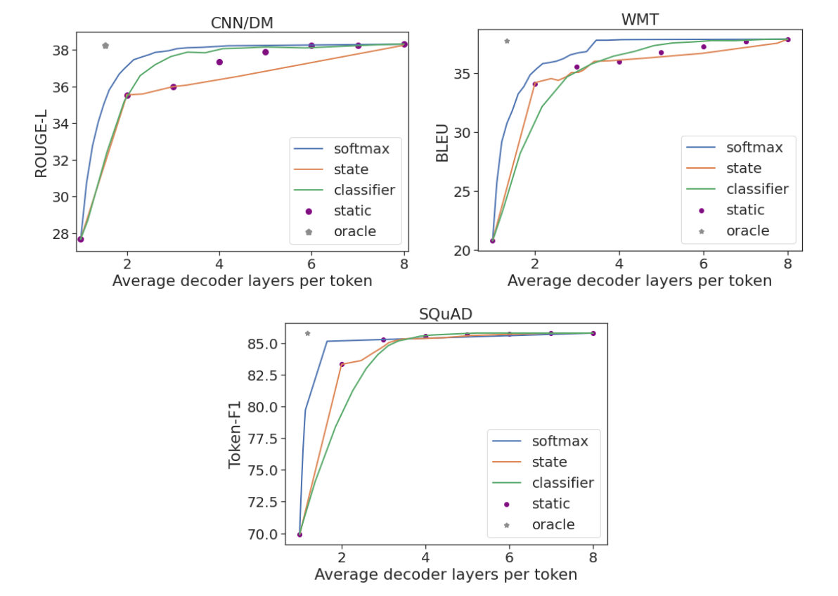
We run experiments on three popular generation datasets: CNN/DM for summarization, WMT for machine translation, and SQuAD for question answering. We evaluate each of the three confidence measures (softmax response, state propagation and early-exit classifier) using an 8-layer encoder-decoder model. To evaluate global sequence-level performance, we use the standard Rouge-L, BLEU, and Token-F1 scores that measure distances against human-written references. We show that one can maintain full model performance while using only a third or half of the layers on average. CALM achieves this by dynamically distributing the compute effort across the prediction timesteps.

As an approximate upper bound, we also compute the predictions using a local oracle confidence measure, which enables exiting at the first layer that leads to the same prediction as the top one. On all three tasks, the oracle measure can preserve full model performance when using only 1.5 decoder layers on average. In contrast to CALM, a static baseline uses the same number of layers for all predictions, requiring 3 to 7 layers (depending on the dataset) to preserve its performance. This demonstrates why the dynamic allocation of compute effort is important. Only a small fraction of the predictions require most of the model’s complexity, while for others much less should suffice.

Performance per task against the average number of decoder layers used.

Finally, we also find that CALM enables practical speedups. When benchmarking on TPUs, we saved almost half of the compute time while maintaining the quality of the outputs.

Example of a generated news summary. The top cell presents the reference human-written summary. Below is the prediction of the full model (8 layers) followed by two different CALM output examples. The first CALM output is 2.9x faster and the second output is 3.6x faster than the full model, benchmarked on TPUs.

Conclusion

CALM allows faster text generation with LMs, without reducing the quality of the output text. This is achieved by dynamically modifying the amount of compute per generation timestep, allowing the model to exit the computational sequence early when confident enough.

As language models continue to grow in size, studying how to efficiently use them becomes crucial. CALM is orthogonal and can be combined with many efficiency related efforts, including model quantization, distillation, sparsity, effective partitioning, and distributed control flows.


Acknowledgements

It was an honor and privilege to work on this with Adam Fisch, Ionel Gog, Seungyeon Kim, Jai Gupta, Mostafa Dehghani, Dara Bahri, Vinh Q. Tran, Yi Tay, and Donald Metzler. We also thank Anselm Levskaya, Hyung Won Chung, Tao Wang, Paul Barham, Michael Isard, Orhan Firat, Carlos Riquelme, Aditya Menon, Zhifeng Chen, Sanjiv Kumar, and Jeff Dean for helpful discussions and feedback. Finally, we thank Tom Small for preparing the animation in this blog post.

Source: Google AI Blog


A Multi-Axis Approach for Vision Transformer and MLP Models

Convolutional neural networks have been the dominant machine learning architecture for computer vision since the introduction of AlexNet in 2012. Recently, inspired by the evolution of Transformers in natural language processing, attention mechanisms have been prominently incorporated into vision models. These attention methods boost some parts of the input data while minimizing other parts so that the network can focus on small but important parts of the data. The Vision Transformer (ViT) has created a new landscape of model designs for computer vision that is completely free of convolution. ViT regards image patches as a sequence of words, and applies a Transformer encoder on top. When trained on sufficiently large datasets, ViT demonstrates compelling performance on image recognition.

While convolutions and attention are both sufficient for good performance, neither of them are necessary. For example, MLP-Mixer adopts a simple multi-layer perceptron (MLP) to mix image patches across all the spatial locations, resulting in an all-MLP architecture. It is a competitive alternative to existing state-of-the-art vision models in terms of the trade-off between accuracy and computation required for training and inference. However, both ViT and the MLP models struggle to scale to higher input resolution because the computational complexity increases quadratically with respect to the image size.

Today we present a new multi-axis approach that is simple and effective, improves on the original ViT and MLP models, can better adapt to high-resolution, dense prediction tasks, and can naturally adapt to different input sizes with high flexibility and low complexity. Based on this approach, we have built two backbone models for high-level and low-level vision tasks. We describe the first in “MaxViT: Multi-Axis Vision Transformer”, to be presented in ECCV 2022, and show it significantly improves the state of the art for high-level tasks, such as image classification, object detection, segmentation, quality assessment, and generation. The second, presented in “MAXIM: Multi-Axis MLP for Image Processing” at CVPR 2022, is based on a UNet-like architecture and achieves competitive performance on low-level imaging tasks including denoising, deblurring, dehazing, deraining, and low-light enhancement. To facilitate further research on efficient Transformer and MLP models, we have open-sourced the code and models for both MaxViT and MAXIM.

A demo of image deblurring using MAXIM frame by frame.

Overview
Our new approach is based on multi-axis attention, which decomposes the full-size attention (each pixel attends to all the pixels) used in ViT into two sparse forms — local and (sparse) global. As shown in the figure below, the multi-axis attention contains a sequential stack of block attention and grid attention. The block attention works within non-overlapping windows (small patches in intermediate feature maps) to capture local patterns, while the grid attention works on a sparsely sampled uniform grid for long-range (global) interactions. The window sizes of grid and block attentions can be fully controlled as hyperparameters to ensure a linear computational complexity to the input size.

The proposed multi-axis attention conducts blocked local and dilated global attention sequentially followed by a FFN, with only a linear complexity. The pixels in the same colors are attended together.

Such low-complexity attention can significantly improve its wide applicability to many vision tasks, especially for high-resolution visual predictions, demonstrating greater generality than the original attention used in ViT. We build two backbone instantiations out of this multi-axis attention approach – MaxViT and MAXIM, for high-level and low-level tasks, respectively.

MaxViT
In MaxViT, we first build a single MaxViT block (shown below) by concatenating MBConv (proposed by EfficientNet, V2) with the multi-axis attention. This single block can encode local and global visual information regardless of input resolution. We then simply stack repeated blocks composed of attention and convolutions in a hierarchical architecture (similar to ResNet, CoAtNet), yielding our homogenous MaxViT architecture. Notably, MaxViT is distinguished from previous hierarchical approaches as it can “see” globally throughout the entire network, even in earlier, high-resolution stages, demonstrating stronger model capacity on various tasks.

The meta-architecture of MaxViT.

MAXIM
Our second backbone, MAXIM, is a generic UNet-like architecture tailored for low-level image-to-image prediction tasks. MAXIM explores parallel designs of the local and global approaches using the gated multi-layer perceptron (gMLP) network (patching-mixing MLP with a gating mechanism). Another contribution of MAXIM is the cross-gating block that can be used to apply interactions between two different input signals. This block can serve as an efficient alternative to the cross-attention module as it only employs the cheap gated MLP operators to interact with various inputs without relying on the computationally heavy cross-attention. Moreover, all the proposed components including the gated MLP and cross-gating blocks in MAXIM enjoy linear complexity to image size, making it even more efficient when processing high-resolution pictures.

Results
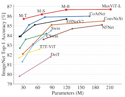
We demonstrate the effectiveness of MaxViT on a broad range of vision tasks. On image classification, MaxViT achieves state-of-the-art results under various settings: with only ImageNet-1K training, MaxViT attains 86.5% top-1 accuracy; with ImageNet-21K (14M images, 21k classes) pre-training, MaxViT achieves 88.7% top-1 accuracy; and with JFT (300M images, 18k classes) pre-training, our largest model MaxViT-XL achieves a high accuracy of 89.5% with 475M parameters.

Performance comparison of MaxViT with state-of-the-art models on ImageNet-1K. Top: Accuracy vs. FLOPs performance scaling with 224x224 image resolution. Bottom: Accuracy vs. parameters scaling curve under ImageNet-1K fine-tuning setting.

For downstream tasks, MaxViT as a backbone delivers favorable performance on a broad spectrum of tasks. For object detection and segmentation on the COCO dataset, the MaxViT backbone achieves 53.4 AP, outperforming other base-level models while requiring only about 60% the computational cost. For image aesthetics assessment, the MaxViT model advances the state-of-the-art MUSIQ model by 3.5% in terms of linear correlation with human opinion scores. The standalone MaxViT building block also demonstrates effective performance on image generation, achieving better FID and IS scores on the ImageNet-1K unconditional generation task with a significantly lower number of parameters than the state-of-the-art model, HiT.

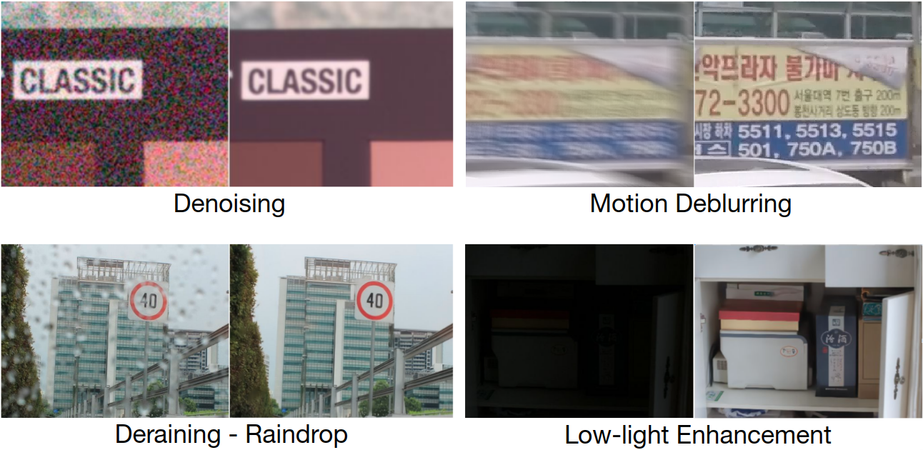
The UNet-like MAXIM backbone, customized for image processing tasks, has also demonstrated state-of-the-art results on 15 out of 20 tested datasets, including denoising, deblurring, deraining, dehazing, and low-light enhancement, while requiring fewer or comparable number of parameters and FLOPs than competitive models. Images restored by MAXIM show more recovered details with less visual artifacts.

Visual results of MAXIM for image deblurring, deraining, and low-light enhancement.

Summary
Recent works in the last two or so years have shown that ConvNets and Vision Transformers can achieve similar performance. Our work presents a unified design that takes advantage of the best of both worlds — efficient convolution and sparse attention — and demonstrates that a model built on top, namely MaxViT, can achieve state-of-the-art performance on a variety of vision tasks. More importantly, MaxViT scales well to very large data sizes. We also show that an alternative multi-axis design using MLP operators, MAXIM, achieves state-of-the-art performance on a broad range of low-level vision tasks.

Even though we present our models in the context of vision tasks, the proposed multi-axis approach can easily extend to language modeling to capture both local and global dependencies in linear time. Motivated by the work here, we expect that it is worthwhile to study other forms of sparse attention in higher-dimensional or multimodal signals such as videos, point clouds, and vision-language models.

We have open-sourced the code and models of MAXIM and MaxViT to facilitate future research on efficient attention and MLP models.

Acknowledgments
We would like to thank our co-authors: Hossein Talebi, Han Zhang, Feng Yang, Peyman Milanfar, and Alan Bovik. We would also like to acknowledge the valuable discussion and support from Xianzhi Du, Long Zhao, Wuyang Chen, Hanxiao Liu, Zihang Dai, Anurag Arnab, Sungjoon Choi, Junjie Ke, Mauricio Delbracio, Irene Zhu, Innfarn Yoo, Huiwen Chang, and Ce Liu.

Source: Google AI Blog


Enhancing Backpropagation via Local Loss Optimization

While model design and training data are key ingredients in a deep neural network’s (DNN’s) success, less-often discussed is the specific optimization method used for updating the model parameters (weights). Training DNNs involves minimizing a loss function that measures the discrepancy between the ground truth labels and the model’s predictions. Training is carried out by backpropagation, which adjusts the model weights via gradient descent steps. Gradient descent, in turn, updates the weights by using the gradient (i.e., derivative) of the loss with respect to the weights.

The simplest weight update corresponds to stochastic gradient descent, which, in every step, moves the weights in the negative direction with respect to the gradients (with an appropriate step size, a.k.a. the learning rate). More advanced optimization methods modify the direction of the negative gradient before updating the weights by using information from the past steps and/or the local properties (such as the curvature information) of the loss function around the current weights. For instance, a momentum optimizer encourages moving along the average direction of past updates, and the AdaGrad optimizer scales each coordinate based on the past gradients. These optimizers are commonly known as first-order methods since they generally modify the update direction using only information from the first-order derivative (i.e., gradient). More importantly, the components of the weight parameters are treated independently from each other.

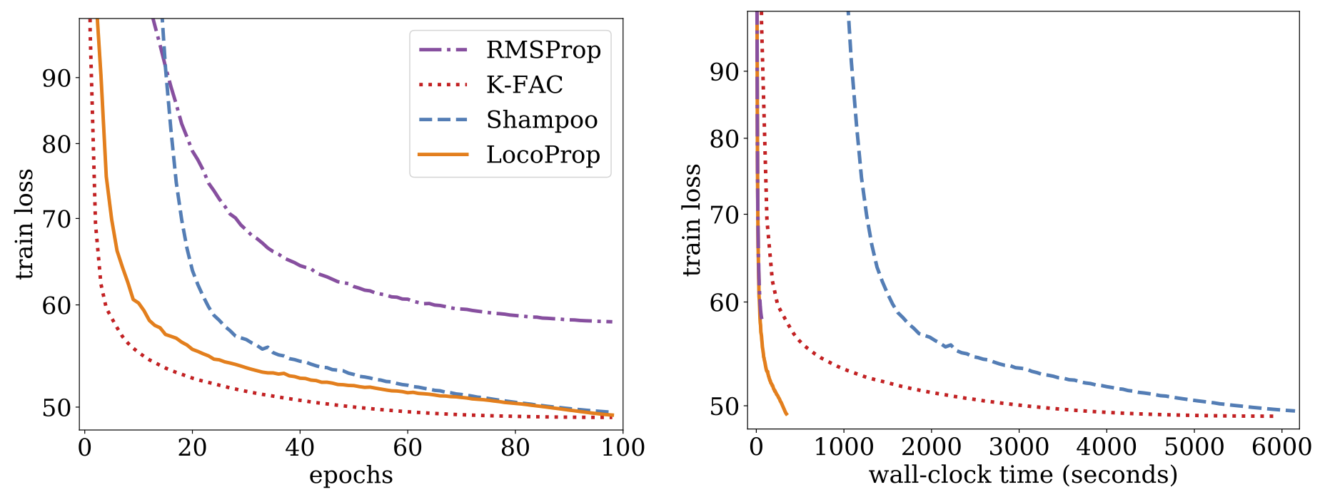
More advanced optimization, such as Shampoo and K-FAC, capture the correlations between gradients of parameters and have been shown to improve convergence, reducing the number of iterations and improving the quality of the solution. These methods capture information about the local changes of the derivatives of the loss, i.e., changes in gradients. Using this additional information, higher-order optimizers can discover much more efficient update directions for training models by taking into account the correlations between different groups of parameters. On the downside, calculating higher-order update directions is computationally more expensive than first-order updates. The operation uses more memory for storing statistics and involves matrix inversion, thus hindering the applicability of higher-order optimizers in practice.

In “LocoProp: Enhancing BackProp via Local Loss Optimization”, we introduce a new framework for training DNN models. Our new framework, LocoProp, conceives neural networks as a modular composition of layers. Generally, each layer in a neural network applies a linear transformation on its inputs, followed by a non-linear activation function. In the new construction, each layer is allotted its own weight regularizer, output target, and loss function. The loss function of each layer is designed to match the activation function of the layer. Using this formulation, training minimizes the local losses for a given mini-batch of examples, iteratively and in parallel across layers. Our method performs multiple local updates per batch of examples using a first-order optimizer (like RMSProp), which avoids computationally expensive operations such as the matrix inversions required for higher-order optimizers. However, we show that the combined local updates look rather like a higher-order update. Empirically, we show that LocoProp outperforms first-order methods on a deep autoencoder benchmark and performs comparably to higher-order optimizers, such as Shampoo and K-FAC, without the high memory and computation requirements.

Method
Neural networks are generally viewed as composite functions that transform model inputs into output representations, layer by layer. LocoProp adopts this view while decomposing the network into layers. In particular, instead of updating the weights of the layer to minimize the loss function at the output, LocoProp applies pre-defined local loss functions specific to each layer. For a given layer, the loss function is selected to match the activation function, e.g., a tanh loss would be selected for a layer with a tanh activation. Each layerwise loss measures the discrepancy between the layer's output (for a given mini-batch of examples) and a notion of a target output for that layer. Additionally, a regularizer term ensures that the updated weights do not drift too far from the current values. The combined layerwise loss function (with a local target) plus regularizer is used as the new objective function for each layer.
Similar to backpropagation, LocoProp applies a forward pass to compute the activations. In the backward pass, LocoProp sets per neuron "targets" for each layer. Finally, LocoProp splits model training into independent problems across layers where several local updates can be applied to each layer's weights in parallel.

Perhaps the simplest loss function one can think of for a layer is the squared loss. While the squared loss is a valid choice of a loss function, LocoProp takes into account the possible non-linearity of the activation functions of the layers and applies layerwise losses tailored to the activation function of each layer. This enables the model to emphasize regions at the input that are more important for the model prediction while deemphasizing the regions that do not affect the output as much. Below we show examples of tailored losses for the tanh and ReLU activation functions.

Loss functions induced by the (left) tanh and (right) ReLU activation functions. Each loss is more sensitive to the regions affecting the output prediction. For instance, ReLU loss is zero as long as both the prediction (â) and the target (a) are negative. This is because the ReLU function applied to any negative number equals zero.

After forming the objective in each layer, LocoProp updates the layer weights by repeatedly applying gradient descent steps on its objective. The update typically uses a first-order optimizer (like RMSProp). However, we show that the overall behavior of the combined updates closely resembles higher-order updates (shown below). Thus, LocoProp provides training performance close to what higher-order optimizers achieve without the high memory or computation needed for higher-order methods, such as matrix inverse operations. We show that LocoProp is a flexible framework that allows the recovery of well-known algorithms and enables the construction of new algorithms via different choices of losses, targets, and regularizers. LocoProp’s layerwise view of neural networks also allows updating the weights in parallel across layers.

Experiments
In our paper, we describe experiments on the deep autoencoder model, which is a commonly used baseline for evaluating the performance of optimization algorithms. We perform extensive tuning on multiple commonly used first-order optimizers, including SGD, SGD with momentum, AdaGrad, RMSProp, and Adam, as well as the higher-order Shampoo and K-FAC optimizers, and compare the results with LocoProp. Our findings indicate that the LocoProp method performs significantly better than first-order optimizers and is comparable to those of higher-order, while being significantly faster when run on a single GPU.

Train loss vs. number of epochs (left) and wall-clock time, i.e., the real time that passes during training, (right) for RMSProp, Shampoo, K-FAC, and LocoProp on the deep autoencoder model.

Summary and Future Directions
We introduced a new framework, called LocoProp, for optimizing deep neural networks more efficiently. LocoProp decomposes neural networks into separate layers with their own regularizer, output target, and loss function and applies local updates in parallel to minimize the local objectives. While using first-order updates for the local optimization problems, the combined updates closely resemble higher-order update directions, both theoretically and empirically.

LocoProp provides flexibility to choose the layerwise regularizers, targets, and loss functions. Thus, it allows the development of new update rules based on these choices. Our code for LocoProp is available online on GitHub. We are currently working on scaling up ideas induced by LocoProp to much larger scale models; stay tuned!

Acknowledgments
We would like to thank our co-author, Manfred K. Warmuth, for his critical contributions and inspiring vision. We would like to thank Sameer Agarwal for discussions looking at this work from a composite functions perspective, Vineet Gupta for discussions and development of Shampoo, Zachary Nado on K-FAC, Tom Small for development of the animation used in this blogpost and finally, Yonghui Wu and Zoubin Ghahramani for providing us with a nurturing research environment in the Google Brain Team.

Source: Google AI Blog