Author Archives: Google AI

Navigating Recorder Transcripts Easily, with Smart Scrolling

Last year we launched Recorder, a new kind of recording app that made audio recording smarter and more useful by leveraging on-device machine learning (ML) to transcribe the recording, highlight audio events, and suggest appropriate tags for titles. Recorder makes editing, sharing and searching through transcripts easier. Yet because Recorder can transcribe very long recordings (up to 18 hours!), it can still be difficult for users to find specific sections, necessitating a new solution to quickly navigate such long transcripts.

To increase the navigability of content, we introduce Smart Scrolling, a new ML-based feature in Recorder that automatically marks important sections in the transcript, chooses the most representative keywords from each section, and then surfaces those keywords on the vertical scrollbar, like chapter headings. The user can then scroll through the keywords or tap on them to quickly navigate to the sections of interest. The models used are lightweight enough to be executed on-device without the need to upload the transcript, thus preserving user privacy.

Smart Scrolling feature UX

Under the hood
The Smart Scrolling feature is composed of two distinct tasks. The first extracts representative keywords from each section and the second picks which sections in the text are the most informative and unique.

For each task, we utilize two different natural language processing (NLP) approaches: a distilled bidirectional transformer (BERT) model pre-trained on data sourced from a Wikipedia dataset, alongside a modified extractive term frequency–inverse document frequency (TF-IDF) model. By using the bidirectional transformer and the TF-IDF-based models in parallel for both the keyword extraction and important section identification tasks, alongside aggregation heuristics, we were able to harness the advantages of each approach and mitigate their respective drawbacks (more on this in the next section).

The bidirectional transformer is a neural network architecture that employs a self-attention mechanism to achieve context-aware processing of the input text in a non-sequential fashion. This enables parallel processing of the input text to identify contextual clues both before and after a given position in the transcript.

Bidirectional Transformer-based model architecture

The extractive TF-IDF approach rates terms based on their frequency in the text compared to their inverse frequency in the trained dataset, and enables the finding of unique representative terms in the text.

Both models were trained on publicly available conversational datasets that were labeled and evaluated by independent raters. The conversational datasets were from the same domains as the expected product use cases, focusing on meetings, lectures, and interviews, thus ensuring the same word frequency distribution (Zipf’s law).

Extracting Representative Keywords
The TF-IDF-based model detects informative keywords by giving each word a score, which corresponds to how representative this keyword is within the text. The model does so, much like a standard TF-IDF model, by utilizing the ratio of the number of occurrences of a given word in the text compared to the whole of the conversational data set, but it also takes into account the specificity of the term, i.e., how broad or specific it is. Furthermore, the model then aggregates these features into a score using a pre-trained function curve. In parallel, the bidirectional transformer model, which was fine tuned on the task of extracting keywords, provides a deep semantic understanding of the text, enabling it to extract precise context-aware keywords.

The TF-IDF approach is conservative in the sense that it is prone to finding uncommon keywords in the text (high bias), while the drawback for the bidirectional transformer model is the high variance of the possible keywords that can be extracted. But when used together, these two models complement each other, forming a balanced bias-variance tradeoff.

Once the keyword scores are retrieved from both models, we normalize and combine them by utilizing NLP heuristics (e.g., the weighted average), removing duplicates across sections, and eliminating stop words and verbs. The output of this process is an ordered list of suggested keywords for each of the sections.

Rating A Section’s Importance
The next task is to determine which sections should be highlighted as informative and unique. To solve this task, we again combine the two models mentioned above, which yield two distinct importance scores for each of the sections. We compute the first score by taking the TF-IDF scores of all the keywords in the section and weighting them by their respective number of appearances in the section, followed by a summation of these individual keyword scores. We compute the second score by running the section text through the bidirectional transformer model, which was also trained on the sections rating task. The scores from both models are normalized and then combined to yield the section score.

Smart Scrolling pipeline architecture

Some Challenges
A significant challenge in the development of Smart Scrolling was how to identify whether a section or keyword is important - what is of great importance to one person can be of less importance to another. The key was to highlight sections only when it is possible to extract helpful keywords from them.

To do this, we configured the solution to select the top scored sections that also have highly rated keywords, with the number of sections highlighted proportional to the length of the recording. In the context of the Smart Scrolling features, a keyword was more highly rated if it better represented the unique information of the section.

To train the model to understand this criteria, we needed to prepare a labeled training dataset tailored to this task. In collaboration with a team of skilled raters, we applied this labeling objective to a small batch of examples to establish an initial dataset in order to evaluate the quality of the labels and instruct the raters in cases where there were deviations from what was intended. Once the labeling process was complete we reviewed the labeled data manually and made corrections to the labels as necessary to align them with our definition of importance.

Using this limited labeled dataset, we ran automated model evaluations to establish initial metrics on model quality, which were used as a less-accurate proxy to the model quality, enabling us to quickly assess the model performance and apply changes in the architecture and heuristics. Once the solution metrics were satisfactory, we utilized a more accurate manual evaluation process over a closed set of carefully chosen examples that represented expected Recorder use cases. Using these examples, we tweaked the model heuristics parameters to reach the desired level of performance using a reliable model quality evaluation.

Runtime Improvements
After the initial release of Recorder, we conducted a series of user studies to learn how to improve the usability and performance of the Smart Scrolling feature. We found that many users expect the navigational keywords and highlighted sections to be available as soon as the recording is finished. Because the computation pipeline described above can take a considerable amount of time to compute on long recordings, we devised a partial processing solution that amortizes this computation over the whole duration of the recording. During recording, each section is processed as soon as it is captured, and then the intermediate results are stored in memory. When the recording is done, Recorder aggregates the intermediate results.

When running on a Pixel 5, this approach reduced the average processing time of an hour long recording (~9K words) from 1 minute 40 seconds to only 9 seconds, while outputting the same results.

Summary
The goal of Recorder is to improve users’ ability to access their recorded content and navigate it with ease. We have already made substantial progress in this direction with the existing ML features that automatically suggest title words for recordings and enable users to search recordings for sounds and text. Smart Scrolling provides additional text navigation abilities that will further improve the utility of Recorder, enabling users to rapidly surface sections of interest, even for long recordings.

Acknowledgments
Bin Zhang, Sherry Lin, Isaac Blankensmith, Henry Liu‎, Vincent Peng‎, Guilherme Santos‎, Tiago Camolesi, Yitong Lin, James Lemieux, Thomas Hall‎, Kelly Tsai‎, Benny Schlesinger, Dror Ayalon, Amit Pitaru, Kelsie Van Deman, Console Chen, Allen Su, Cecile Basnage, Chorong Johnston‎, Shenaz Zack, Mike Tsao, Brian Chen, Abhinav Rastogi, Tracy Wu, Yvonne Yang‎.

Source: Google AI Blog


The Language Interpretability Tool (LIT): Interactive Exploration and Analysis of NLP Models

As natural language processing (NLP) models become more powerful and are deployed in more real-world contexts, understanding their behavior is becoming increasingly critical. While advances in modeling have brought unprecedented performance on many NLP tasks, many research questions remain about not only the behavior of these models under domain shift and adversarial settings, but also their tendencies to behave according to social biases or shallow heuristics.

For any new model, one might want to know in which cases a model performs poorly, why a model makes a particular prediction, or whether a model will behave consistently under varying inputs, such as changes to textual style or pronoun gender. But, despite the recent explosion of work on model understanding and evaluation, there is no “silver bullet” for analysis. Practitioners must often experiment with many techniques, looking at local explanations, aggregate metrics, and counterfactual variations of the input to build a better understanding of model behavior, with each of these techniques often requiring its own software package or bespoke tool. Our previously released What-If Tool was built to address this challenge by enabling black-box probing of classification and regression models, thus enabling researchers to more easily debug performance and analyze the fairness of machine learning models through interaction and visualization. But there was still a need for a toolkit that would address challenges specific to NLP models.

With these challenges in mind, we built and open-sourced the Language Interpretability Tool (LIT), an interactive platform for NLP model understanding. LIT builds upon the lessons learned from the What-If Tool with greatly expanded capabilities, which cover a wide range of NLP tasks including sequence generation, span labeling, classification and regression, along with customizable and extensible visualizations and model analysis.

LIT supports local explanations, including salience maps, attention, and rich visualizations of model predictions, as well as aggregate analysis including metrics, embedding spaces, and flexible slicing. It allows users to easily hop between visualizations to test local hypotheses and validate them over a dataset. LIT provides support for counterfactual generation, in which new data points can be added on the fly, and their effect on the model visualized immediately. Side-by-side comparison allows for two models, or two individual data points, to be visualized simultaneously. More details about LIT can be found in our system demonstration paper, which was presented at EMNLP 2020.

Exploring a sentiment classifier with LIT.

Customizability
In order to better address the broad range of users with different interests and priorities that we hope will use LIT, we’ve built the tool to be easily customizable and extensible from the start. Using LIT on a particular NLP model and dataset only requires writing a small bit of Python code. Custom components, such as task-specific metrics calculations or counterfactual generators, can be written in Python and added to a LIT instance through our provided APIs. Also, the front end itself can be customized, with new modules that integrate directly into the UI. For more on extending the tool, check out our documentation on GitHub.

Demos
To illustrate some of the capabilities of LIT, we have created a few demos using pre-trained models. The full list is available on the LIT website, and we describe two of them here:

  • Sentiment analysis: In this example, a user can explore a BERT-based binary classifier that predicts if a sentence has positive or negative sentiment. The demo uses the Stanford Sentiment Treebank of sentences from movie reviews to demonstrate model behavior. One can examine local explanations using saliency maps provided by a variety of techniques (such as LIME and integrated gradients), and can test model behavior with perturbed (counterfactual) examples using techniques such as back-translation, word replacement, or adversarial attacks. These techniques can help pinpoint under what scenarios a model fails, and whether those failures are generalizable, which can then be used to inform how best to improve a model.
    Analyzing token-based salience of an incorrect prediction. The word “laughable” seems to be incorrectly raising the positive sentiment score of this example.
  • Masked word prediction: Masked language modeling is a "fill-in-the-blank" task, where the model predicts different words that could complete a sentence. For example, given the prompt, "I took my ___ for a walk", the model might predict a high score for "dog." In LIT one can explore this interactively by typing in sentences or choosing from a pre-loaded corpus, and then clicking specific tokens to see what a model like BERT understands about language, or about the world.
    Interactively selecting a token to mask, and viewing a language model's predictions.

LIT in Practice and Future Work
Although LIT is a new tool, we have already seen the value that it can provide for model understanding. Its visualizations can be used to find patterns in model behavior, such as outlying clusters in embedding space, or words with outsized importance to the predictions. Exploration in LIT can test for potential biases in models, as demonstrated in our case study of LIT exploring gender bias in a coreference model. This type of analysis can inform next steps in improving model performance, such as applying MinDiff to mitigate systemic bias. It can also be used as an easy and fast way to create an interactive demo for any NLP model.

Check out the tool either through our provided demos, or by bringing up a LIT server for your own models and datasets. The work on LIT has just started, and there are a number of new capabilities and refinements planned, including the addition of new interpretability techniques from cutting edge ML and NLP research. If there are other techniques that you’d like to see added to the tool, please let us know! Join our mailing list to stay up to date as LIT evolves. And as the code is open-source, we welcome feedback on and contributions to the tool.

Acknowledgments
LIT is a collaborative effort between the Google Research PAIR and Language teams. This post represents the work of the many contributors across Google, including Andy Coenen, Ann Yuan, Carey Radebaugh, Ellen Jiang, Emily Reif, Jasmijn Bastings, Kristen Olson, Leslie Lai, Mahima Pushkarna, Sebastian Gehrmann, and Tolga Bolukbasi. We would like to thank all those who contributed to the project, both inside and outside Google, and the teams that have piloted its use and provided valuable feedback.

Source: Google AI Blog


Haptics with Input: Using Linear Resonant Actuators for Sensing

As wearables and handheld devices decrease in size, haptics become an increasingly vital channel for feedback, be it through silent alerts or a subtle "click" sensation when pressing buttons on a touch screen. Haptic feedback, ubiquitous in nearly all wearable devices and mobile phones, is commonly enabled by a linear resonant actuator (LRA), a small linear motor that leverages resonance to provide a strong haptic signal in a small package. However, the touch and pressure sensing needed to activate the haptic feedback tend to depend on additional, separate hardware which increases the price, size and complexity of the system.

In “Haptics with Input: Back-EMF in Linear Resonant Actuators to Enable Touch, Pressure and Environmental Awareness”, presented at ACM UIST 2020, we demonstrate that widely available LRAs can sense a wide range of external information, such as touch, tap and pressure, in addition to being able to relay information about contact with the skin, objects and surfaces. We achieve this with off-the-shelf LRAs by multiplexing the actuation with short pulses of custom waveforms that are designed to enable sensing using the back-EMF voltage. We demonstrate the potential of this approach to enable expressive discrete buttons and vibrotactile interfaces and show how the approach could bring rich sensing opportunities to integrated haptics modules in mobile devices, increasing sensing capabilities with fewer components. Our technique is potentially compatible with many existing LRA drivers, as they already employ back-EMF sensing for autotuning of the vibration frequency.

Different off-the-shelf LRAs that work using this technique.

Back-EMF Principle in an LRA
Inside the LRA enclosure is a magnet attached to a small mass, both moving freely on a spring. The magnet moves in response to the excitation voltage introduced by the voice coil. The motion of the oscillating mass produces a counter-electromotive force, or back-EMF, which is a voltage proportional to the rate of change of magnetic flux. A greater oscillation speed creates a larger back-EMF voltage, while a stationary mass generates zero back-EMF voltage.

Anatomy of the LRA.

Active Back-EMF for Sensing
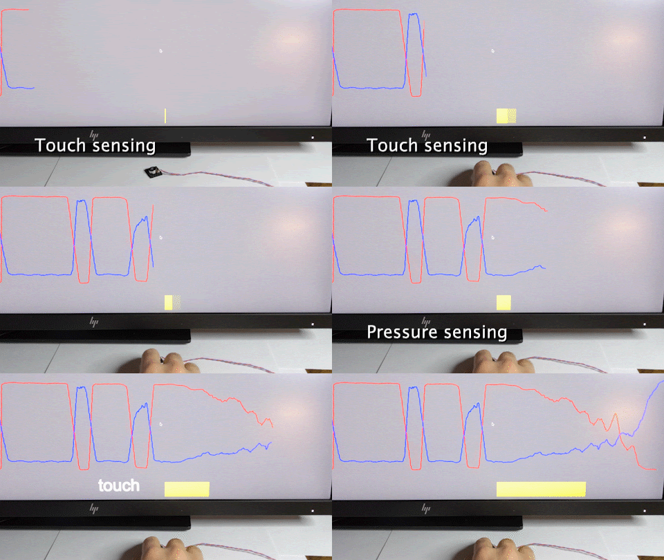
Touching or making contact with the LRA during vibration changes the velocity of the interior mass, as energy is dissipated into the contact object. This works well with soft materials that deform under pressure, such as the human body. A finger, for example, absorbs different amounts of energy depending on the contact force as it flattens against the LRA. By driving the LRA with small amounts of energy, we can measure this phenomenon using the back-EMF voltage. Because leveraging the back-EMF behavior for sensing is an active process, the key insight that enabled this work was the design of a custom, off-resonance driver waveform that allows continuous sensing while minimizing vibrations, sound and power consumption.

Touch and pressure sensing on the LRA.

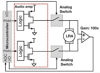
We measure back-EMF from the floating voltage between the two LRA leads, which requires disconnecting the motor driver briefly to avoid disturbances. While the driver is disconnected, the mass is still oscillating inside the LRA, producing an oscillating back-EMF voltage. Because commercial back-EMF sensing LRA drivers do not provide the raw data, we designed a custom circuit that is able to pick up and amplify small back-EMF voltage. We also generated custom drive pulses that minimize vibrations and energy consumption.

Simplified schematic of the LRA driver and the back-EMF measurement circuit for active sensing.
After exciting the LRA with a short drive pulse, the back-EMF voltage fluctuates due to the continued oscillations of the mass on the spring (top, red line). The change in the back-EMF signal when subject to a finger press depends on the pressure applied (middle/bottom, green/blue lines).

Applications
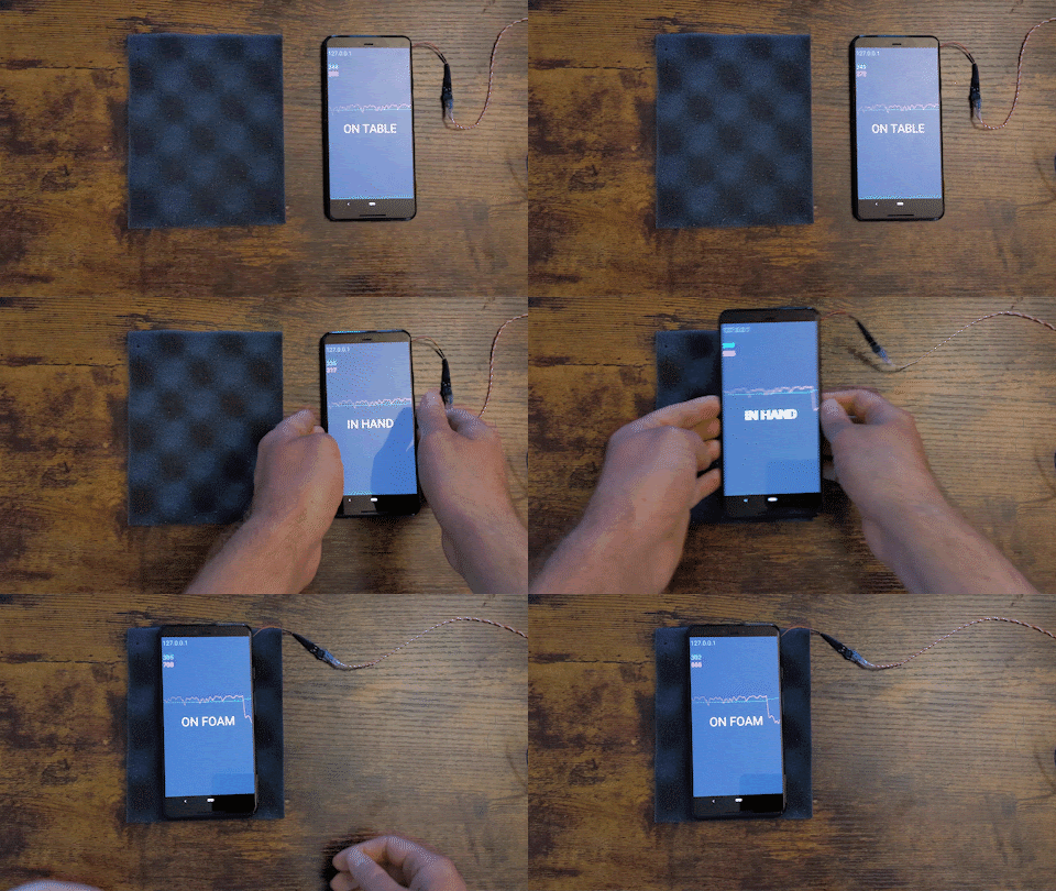
The behavior of the LRAs used in mobile phones is the same, whether they are on a table, on a soft surface, or hand held. This may cause problems, as a vibrating phone could slide off a glass table or emit loud and unnecessary vibrating sounds. Ideally, the LRA on a phone would automatically adjust based on its environment. We demonstrate our approach for sensing using the LRA back-EMF technique by wiring directly to a Pixel 4’s LRA, and then classifying whether the phone is held in hand, placed on a soft surface (foam), or placed on a table.

Sensing phone surroundings.

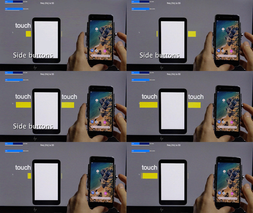
We also present a prototype that demonstrates how LRAs could be used as combined input/output devices in portable electronics. We attached two LRAs, one on the left and one on the right side of a phone. The buttons provide tap, touch, and pressure sensing. They are also programmed to provide haptic feedback, once the touch is detected.

Pressure-sensitive side buttons.

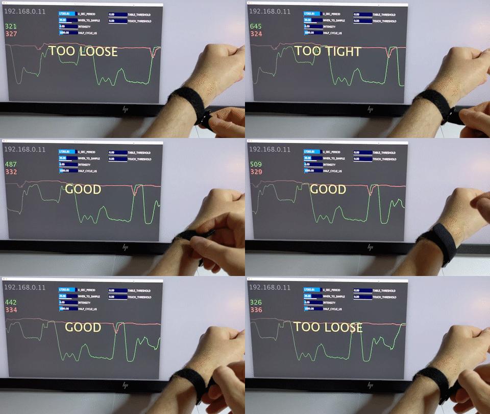
There are a number of wearable tactile aid devices, such as sleeves, vests, and bracelets. To transmit tactile feedback to the skin with consistent force, the tactor has to apply the right pressure; it can not be too loose or too tight. Currently, the typical way to do so is through manual adjustment, which can be inconsistent and lacks measurable feedback. We show how the LRA back-EMF technique can be used to continuously monitor the fit bracelet device and prompt the user if it's too tight, too loose, or just right.

Fit sensing bracelet.

Evaluating an LRA as a Sensor
The LRA works well as a pressure sensor, because it has a quadratic response to the force magnitude during touch. Our method works for all five off-the-shelf LRA types that we evaluated. Because the typical power consumption is only 4.27 mA, all-day sensing would only reduce the battery life of a Pixel 4 phone from 25 to 24 hours. The power consumption can be greatly reduced by using low-power amplifiers and employing active sensing only when needed, such as when the phone is active and interacting with the user.

Back-EMF voltage changes when pressure is applied with a finger.

The challenge with active sensing is to minimize vibrations, so they are not perceptible when touching and do not produce audible sound. We optimize the active sensing to produce only 2 dB of sound and 0.45 m/s2 peak-to-peak acceleration, which is just barely perceptible by finger and is quiet, in contrast to the regular 8.49 m/s2 .

Future Work and Conclusion
To see the work presented here in action, please see the video below.

In the future, we plan to explore other sensing techniques, perhaps measuring the current could be an alternative approach. Also, using machine learning could potentially improve the sensing and provide more accurate classification of the complex back-EMF patterns. Our method could be developed further to enable closed-loop feedback with the actuator and sensor, which would allow the actuator to provide the same force, regardless of external conditions.

We believe that this work opens up new opportunities for leveraging existing ubiquitous hardware to provide rich interactions and closed-loop feedback haptic actuators.

Acknowledgments
This work was done by Artem Dementyev, Alex Olwal, and Richard Lyon. Thanks to Mathieu Le Goc and Thad Starner for feedback on the paper.

Source: Google AI Blog


Using GANs to Create Fantastical Creatures

Creating art for digital video games takes a high degree of artistic creativity and technical knowledge, while also requiring game artists to quickly iterate on ideas and produce a high volume of assets, often in the face of tight deadlines. What if artists had a paintbrush that acted less like a tool and more like an assistant? A machine learning model acting as such a paintbrush could reduce the amount of time necessary to create high-quality art without sacrificing artistic choices, perhaps even enhancing creativity.

Today, we present Chimera Painter, a trained machine learning (ML) model that automatically creates a fully fleshed out rendering from a user-supplied creature outline. Employed as a demo application, Chimera Painter adds features and textures to a creature outline segmented with body part labels, such as “wings” or “claws”, when the user clicks the “transform” button. Below is an example using the demo with one of the preset creature outlines.

Using an image imported to Chimera Painter or generated with the tools provided, an artist can iteratively construct or modify a creature outline and use the ML model to generate realistic looking surface textures. In this example, an artist (Lee Dotson) customizes one of the creature designs that comes pre-loaded in the Chimera Painter demo.

In this post, we describe some of the challenges in creating the ML model behind Chimera Painter and demonstrate how one might use the tool for the creation of video game-ready assets.

Prototyping for a New Type of Model
In developing an ML model to produce video-game ready creature images, we created a digital card game prototype around the concept of combining creatures into new hybrids that can then battle each other. In this game, a player would begin with cards of real-world animals (e.g., an axolotl or a whale) and could make them more powerful by combining them (making the dreaded Axolotl-Whale chimera). This provided a creative environment for demonstrating an image-generating model, as the number of possible chimeras necessitated a method for quickly designing large volumes of artistic assets that could be combined naturally, while still retaining identifiable visual characteristics of the original creatures.

Since our goal was to create high-quality creature card images guided by artist input, we experimented with generative adversarial networks (GANs), informed by artist feedback, to create creature images that would be appropriate for our fantasy card game prototype. GANs pair two convolutional neural networks against each other: a generator network to create new images and a discriminator network to determine if these images are samples from the training dataset (in this case, artist-created images) or not. We used a variant called a conditional GAN, where the generator takes a separate input to guide the image generation process. Interestingly, our approach was a strict departure from other GAN efforts, which typically focus on photorealism.

To train the GANs, we created a dataset of full color images with single-species creature outlines adapted from 3D creature models. The creature outlines characterized the shape and size of each creature, and provided a segmentation map that identified individual body parts. After model training, the model was tasked with generating multi-species chimeras, based on outlines provided by artists. The best performing model was then incorporated into Chimera Painter. Below we show some sample assets generated using the model, including single-species creatures, as well as the more complex multi-species chimeras.

Generated card art integrated into the card game prototype showing basic creatures (bottom row) and chimeras from multiple creatures, including an Antlion-Porcupine, Axolotl-Whale, and a Crab-Antion-Moth (top row). More info about the game itself is detailed in this Stadia Research presentation.

Learning to Generate Creatures with Structure
An issue with using GANs for generating creatures was the potential for loss of anatomical and spatial coherence when rendering subtle or low-contrast parts of images, despite these being of high perceptual importance to humans. Examples of this can include eyes, fingers, or even distinguishing between overlapping body parts with similar textures (see the affectionately named BoggleDog below).

GAN-generated image showing mismatched body parts.

Generating chimeras required a new non-photographic fantasy-styled dataset with unique characteristics, such as dramatic perspective, composition, and lighting. Existing repositories of illustrations were not appropriate to use as datasets for training an ML model, because they may be subject to licensing restrictions, have conflicting styles, or simply lack the variety needed for this task.

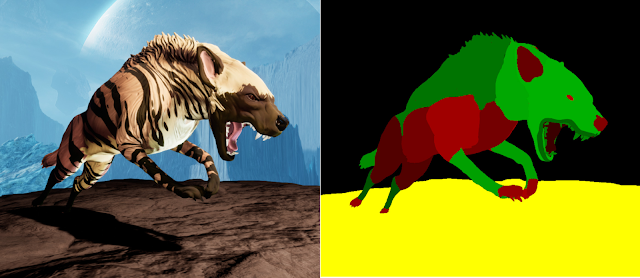
To solve this, we developed a new artist-led, semi-automated approach for creating an ML training dataset from 3D creature models, which allowed us to work at scale and rapidly iterate as needed. In this process, artists would create or obtain a set of 3D creature models, one for each creature type needed (such as hyenas or lions). Artists then produced two sets of textures that were overlaid on the 3D model using the Unreal Engine — one with the full color texture (left image, below) and the other with flat colors for each body part (e.g., head, ears, neck, etc), called a “segmentation map” (right image, below). This second set of body part segments was given to the model at training to ensure that the GAN learned about body part-specific structure, shapes, textures, and proportions for a variety of creatures.

Example dataset training image and its paired segmentation map.

The 3D creature models were all placed in a simple 3D scene, again using the Unreal Engine. A set of automated scripts would then take this 3D scene and interpolate between different poses, viewpoints, and zoom levels for each of the 3D creature models, creating the full color images and segmentation maps that formed the training dataset for the GAN. Using this approach, we generated 10,000+ image + segmentation map pairs per 3D creature model, saving the artists millions of hours of time compared to creating such data manually (at approximately 20 minutes per image).

Fine Tuning
The GAN had many different hyper-parameters that could be adjusted, leading to different qualities in the output images. In order to better understand which versions of the model were better than others, artists were provided samples for different creature types generated by these models and asked to cull them down to a few best examples. We gathered feedback about desired characteristics present in these examples, such as a feeling of depth, style with regard to creature textures, and realism of faces and eyes. This information was used both to train new versions of the model and, after the model had generated hundreds of thousands of creature images, to select the best image from each creature category (e.g., gazelle, lynx, gorilla, etc).

We tuned the GAN for this task by focusing on the perceptual loss. This loss function component (also used in Stadia’s Style Transfer ML) computes a difference between two images using extracted features from a separate convolutional neural network (CNN) that was previously trained on millions of photographs from the ImageNet dataset. The features are extracted from different layers of the CNN and a weight is applied to each, which affects their contribution to the final loss value. We discovered that these weights were critically important in determining what a final generated image would look like. Below are some examples from the GAN trained with different perceptual loss weights.

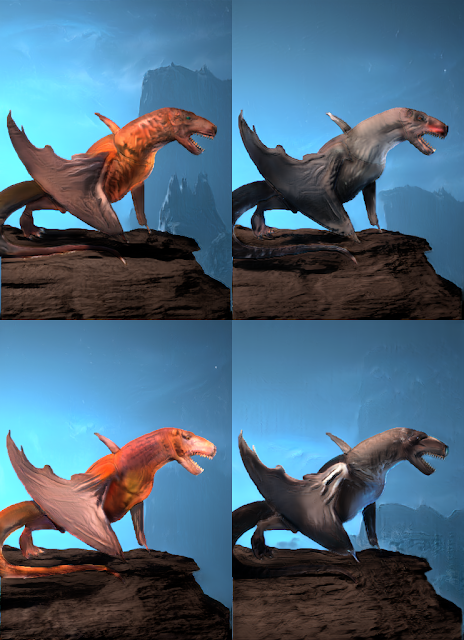
Dino-Bat Chimeras generated using varying perceptual loss weights.

Some of the variation in the images above is due to the fact that the dataset includes multiple textures for each creature (for example, a reddish or grayish version of the bat). However, ignoring the coloration, many differences are directly tied to changes in perceptual loss values. In particular, we found that certain values brought out sharper facial features (e.g., bottom right vs. top right) or “smooth” versus “patterned” (top right vs. bottom left) that made generated creatures feel more real.

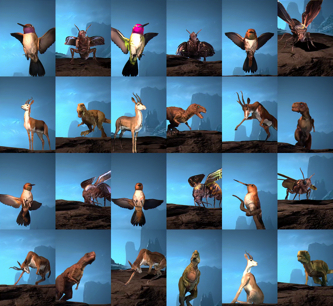
Here are some creatures generated from the GAN trained with different perceptual loss weights, showing off a small sample of the outputs and poses that the model can handle.

Creatures generated using different models.
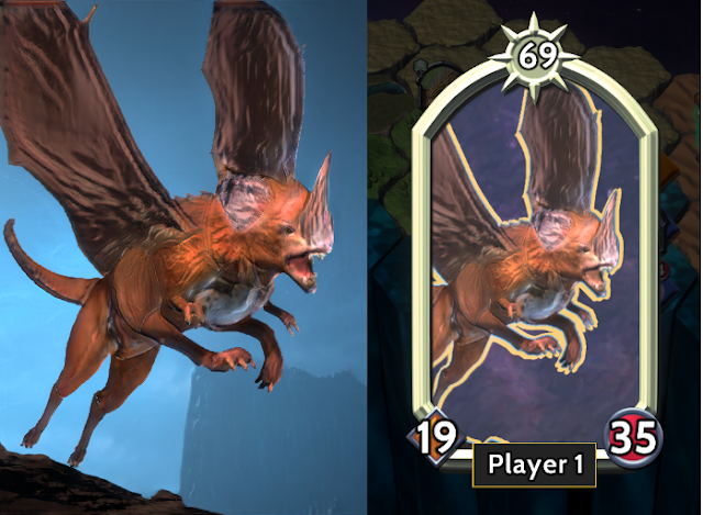
A generated chimera (Dino-Bat-Hyena, to be exact) created using the conditional GAN. Output from the GAN (left) and the post-processed / composited card (right).

Chimera Painter
The trained GAN is now available in the Chimera Painter demo, allowing artists to work iteratively with the model, rather than drawing dozens of similar creatures from scratch. An artist can select a starting point and then adjust the shape, type, or placement of creature parts, enabling rapid exploration and for the creation of a large volume of images. The demo also allows for uploading a creature outline created in an external program, like Photoshop. Simply download one of the preset creature outlines to get the colors needed for each creature part and use this as a template for drawing one outside of Chimera Painter, and then use the “Load’ button on the demo to use this outline to flesh out your creation.

It is our hope that these GAN models and the Chimera Painter demonstration tool might inspire others to think differently about their art pipeline. What can one create when using machine learning as a paintbrush?

Acknowledgments
This project is conducted in collaboration with many people. Thanks to Ryan Poplin, Lee Dotson, Trung Le, Monica Dinculescu, Marc Destefano, Aaron Cammarata, Maggie Oh, Richard Wu, Ji Hun Kim, Erin Hoffman-John, and Colin Boswell. Thanks to everyone who pitched in to give hours of art direction, technical feedback, and drawings of fantastic creatures.

Source: Google AI Blog


Mitigating Unfair Bias in ML Models with the MinDiff Framework

The responsible research and development of machine learning (ML) can play a pivotal role in helping to solve a wide variety of societal challenges. At Google, our research reflects our AI Principles, from helping to protect patients from medication errors and improving flood forecasting models, to presenting methods that tackle unfair bias in products, such as Google Translate, and providing resources for other researchers to do the same.

One broad category for applying ML responsibly is the task of classification — systems that sort data into labeled categories. At Google, such models are used throughout our products to enforce policies, ranging from the detection of hate speech to age-appropriate content filtering. While these classifiers serve vital functions, it is also essential that they are built in ways that minimize unfair biases for users.

Today, we are announcing the release of MinDiff, a new regularization technique available in the TF Model Remediation library for effectively and efficiently mitigating unfair biases when training ML models. In this post, we discuss the research behind this technique and explain how it addresses the practical constraints and requirements we’ve observed when incorporating it in Google’s products.

Unfair Biases in Classifiers
To illustrate how MinDiff can be used, consider an example of a product policy classifier that is tasked with identifying and removing text comments that could be considered toxic. One challenge is to make sure that the classifier is not unfairly biased against submissions from a particular group of users, which could result in incorrect removal of content from these groups.

The academic community has laid a solid theoretical foundation for ML fairness, offering a breadth of perspectives on what unfair bias means and on the tensions between different frameworks for evaluating fairness. One of the most common metrics is equality of opportunity, which, in our example, means measuring and seeking to minimize the difference in false positive rate (FPR) across groups. In the example above, this means that the classifier should not be more likely to incorrectly remove safe comments from one group than another. Similarly, the classifier’s false negative rate should be equal between groups. That is, the classifier should not miss toxic comments against one group more than it does for another.

When the end goal is to improve products, it’s important to be able to scale unfair bias mitigation to many models. However, this poses a number of challenges:

  • Sparse demographic data: The original work on equality of opportunity proposed a post-processing approach to the problem, which consisted of assigning each user group a different classifier threshold at serving time to offset biases of the model. However, in practice this is often not possible for many reasons, such as privacy policies. For example, demographics are often collected by users self-identifying and opting in, but while some users will choose to do this, others may choose to opt-out or delete data. Even for in-process solutions (i.e., methods that change how a model is trained) one needs to assume that most data will not have associated demographics, and thus needs to make efficient use of the few examples for which demographics are known.
  • Ease of Use: In order for any technique to be adopted broadly, it should be easy to incorporate into existing model architectures, and not be highly sensitive to hyperparameters. While an early approach to incorporating ML fairness principles into applications utilized adversarial learning, we found that it too frequently caused models to degenerate during training, which made it difficult for product teams to iterate and made new product teams wary.
  • Quality: The method for removing unfair biases should also reduce the overall classification performance (e.g., accuracy) as little as possible. Because any decrease in accuracy caused by the mitigation approach could result in the moderation model allowing more toxic comments, striking the right balance is crucial.

MinDiff Framework
We iteratively developed the MinDiff framework over the previous few years to meet these design requirements. Because demographic information is so rarely known, we utilize in-process approaches in which the model’s training objective is augmented with an objective specifically focused on removing biases. This new objective is then optimized over the small sample of data with known demographic information. To improve ease of use, we switched from adversarial training to a regularization framework, which penalizes statistical dependency between its predictions and demographic information for non-harmful examples. This encourages the model to equalize error rates across groups, e.g., classifying non-harmful examples as toxic.

There are several ways to encode this dependency between predictions and demographic information. Our initial MinDiff implementation minimized the correlation between the predictions and the demographic group, which essentially optimized for the average and variance of predictions to be equal across groups, even if the distributions still differ afterward. We have since improved MinDiff further by considering the maximum mean discrepancy (MMD) loss, which is closer to optimizing for the distribution of predictions to be independent of demographics. We have found that this approach is better able to both remove biases and maintain model accuracy.

MinDiff with MMD better closes the FPR gap with less decrease in accuracy
(on an academic benchmark dataset).

To date we have launched modeling improvements across several classifiers at Google that moderate content quality. We went through multiple iterations to develop a robust, responsible, and scalable approach, solving research challenges and enabling broad adoption.

Gaps in error rates of classifiers is an important set of unfair biases to address, but not the only one that arises in ML applications. For ML researchers and practitioners, we hope this work can further advance research toward addressing even broader classes of unfair biases and the development of approaches that can be used in practical applications. In addition, we hope that the release of the MinDiff library and the associated demos and documentation, along with the tools and experience shared here, can help practitioners improve their models and products.

Acknowledgements
This research effort on ML Fairness in classification was jointly led with Jilin Chen, Shuo Chen, Ed H. Chi, Tulsee Doshi, and Hai Qian. Further, this work was pursued in collaboration with Jonathan Bischof, Qiuwen Chen, Pierre Kreitmann, and Christine Luu. The MinDiff infrastructure was also developed in collaboration with Nick Blumm, James Chen, Thomas Greenspan, Christina Greer, Lichan Hong, Manasi Joshi, Maciej Kula, Summer Misherghi, Dan Nanas, Sean O'Keefe, Mahesh Sathiamoorthy, Catherina Xu, and Zhe Zhao. (All names are listed in alphabetical order of last names.)

Source: Google AI Blog


The Machine Learning Behind Hum to Search

Melodies stuck in your head, often referred to as “earworms,” are a well-known and sometimes irritating phenomenon — once that earworm is there, it can be tough to get rid of it. Research has found that engaging with the original song, whether that’s listening to or singing it, will drive the earworm away. But what if you can’t quite recall the name of the song, and can only hum the melody?

Existing methods to match a hummed melody to its original polyphonic studio recording face several challenges. With lyrics, background vocals and instruments, the audio of a musical or studio recording can be quite different from a hummed tune. By mistake or design, when someone hums their interpretation of a song, often the pitch, key, tempo or rhythm may vary slightly or even significantly. That’s why so many existing approaches to query by humming match the hummed tune against a database of pre-existing melody-only or hummed versions of a song, instead of identifying the song directly. However, this type of approach often relies on a limited database that requires manual updates.

Launched in October, Hum to Search is a new fully machine-learned system within Google Search that allows a person to find a song using only a hummed rendition of it. In contrast to existing methods, this approach produces an embedding of a melody from a spectrogram of a song without generating an intermediate representation. This enables the model to match a hummed melody directly to the original (polyphonic) recordings without the need for a hummed or MIDI version of each track or for other complex hand-engineered logic to extract the melody. This approach greatly simplifies the database for Hum to Search, allowing it to constantly be refreshed with embeddings of original recordings from across the world — even the latest releases.

Background
Many existing music recognition systems convert an audio sample into a spectrogram before processing it, in order to find a good match. However, one challenge in recognizing a hummed melody is that a hummed tune often contains relatively little information, as illustrated by this hummed example of Bella Ciao. The difference between the hummed version and the same segment from the corresponding studio recording can be visualized using spectrograms, seen below:

Visualization of a hummed clip and a matching studio recording.

Given the image on the left, a model needs to locate the audio corresponding to the right-hand image from a collection of over 50M similar-looking images (corresponding to segments of studio recordings of other songs). To achieve this, the model has to learn to focus on the dominant melody, and ignore background vocals, instruments, and voice timbre, as well as differences stemming from background noise or room reverberations. To find by eye the dominant melody that might be used to match these two spectrograms, a person might look for similarities in the lines near the bottom of the above images.

Prior efforts to enable discovery of music, in particular in the context of recognizing recorded music being played in an environment such as a cafe or a club, demonstrated how machine learning might be applied to this problem. Now Playing, released to Pixel phones in 2017, uses an on-device deep neural network to recognize songs without the need for a server connection, and Sound Search further developed this technology to provide a server-based recognition service for faster and more accurate searching of over 100 million songs. The next challenge then was to leverage what was learned from these releases to recognize hummed or sung music from a similarly large library of songs.

Machine Learning Setup
The first step in developing Hum to Search was to modify the music-recognition models used in Now Playing and Sound Search to work with hummed recordings. In principle, many such retrieval systems (e.g., image recognition) work in a similar way. A neural network is trained with pairs of input (here pairs of hummed or sung audio with recorded audio) to produce embeddings for each input, which will later be used for matching to a hummed melody.

Training setup for the neural network

To enable humming recognition, the network should produce embeddings for which pairs of audio containing the same melody are close to each other, even if they have different instrumental accompaniment and singing voices. Pairs of audio containing different melodies should be far apart. In training, the network is provided such pairs of audio until it learns to produce embeddings with this property.

The trained model can then generate an embedding for a tune that is similar to the embedding of the song’s reference recording. Finding the correct song is then only a matter of searching for similar embeddings from a database of reference recordings computed from audio of popular music.

Training Data
Because training of the model required song pairs (recorded and sung), the first challenge was to obtain enough training data. Our initial dataset consisted of mostly sung music segments (very few of these contained humming). To make the model more robust, we augmented the audio during training, for example by varying the pitch or tempo of the sung input randomly. The resulting model worked well enough for people singing, but not for people humming or whistling.

To improve the model’s performance on hummed melodies we generated additional training data of simulated “hummed” melodies from the existing audio dataset using SPICE, a pitch extraction model developed by our wider team as part of the FreddieMeter project. SPICE extracts the pitch values from given audio, which we then use to generate a melody consisting of discrete audio tones. The very first version of this system transformed this original clip into these tones.

Generating hummed audio from sung audio

We later refined this approach by replacing the simple tone generator with a neural network that generates audio resembling an actual hummed or whistled tune. For example, the network generates this humming example or whistling example from the above sung clip.

As a final step, we compared training data by mixing and matching the audio samples. For example, if we had a similar clip from two different singers, we’d align those two clips with our preliminary models, and are therefore able to show the model an additional pair of audio clips that represent the same melody.

Machine Learning Improvements
When training the Hum to Search model, we started with a triplet loss function. This loss has been shown to perform well across a variety of classification tasks like images and recorded music. Given a pair of audio corresponding to the same melody (points R and P in embedding space, shown below), triplet loss would ignore certain parts of the training data derived from a different melody. This helps the machine improve learning behavior, either when it finds a different melody that is too ‘easy’ in that it is already far away from R and P (see point E) or because it is too hard in that, given the model's current state of learning, the audio ends up being too close to R — even though according to our data it represents a different melody (see point H).

Example audio segments visualized as points in embedding space

We’ve found that we could improve the accuracy of the model by taking these additional training data (points H and E) into account, namely by formulating a general notion of model confidence across a batch of examples: How sure is the model that all the data it has seen can be classified correctly, or has it seen examples that do not fit its current understanding? Based on this notion of confidence, we added a loss that drives model confidence towards 100% across all areas of the embedding space, which led to improvements in our model’s precision and recall.

The above changes, but in particular our variations, augmentations and superpositions of the training data, enabled the neural network model deployed in Google Search to recognize sung or hummed melodies. The current system reaches a high level of accuracy on a song database that contains over half a million songs that we are continually updating. This song corpus still has room to grow to include more of the world’s many melodies.

Hum to Search in the Google App

To try the feature, you can open the latest version of the Google app, tap the mic icon and say “what's this song?” or click the “Search a song” button, after which you can hum, sing, or whistle away! We hope that Hum to Search can help with that earworm of yours, or maybe just help you in case you want to find and playback a song without having to type its name.

Acknowledgements
The work described here was authored by Alex Tudor, Duc Dung Nguyen, Matej Kastelic‎, Mihajlo Velimirović‎, Stefan Christoph, Mauricio Zuluaga, Christian Frank, Dominik Roblek, and Matt Sharifi. We would like to deeply thank Krishna Kumar, Satyajeet Salgar and Blaise Aguera y Arcas for their ongoing support, as well as all the Google teams we've collaborated with to build the full Hum to Search product.

We would also like to thank all our colleagues at Google who donated clips of themselves singing or humming and therefore laid a foundation for this work, as well as Nick Moukhine‎ for building the Google-internal singing donation app. Finally, special thanks to Meghan Danks and Krishna Kumar for their feedback on earlier versions of this post.

Source: Google AI Blog


Improving On-Device Speech Recognition with VoiceFilter-Lite

Voice assistive technologies, which enable users to employ voice commands to interact with their devices, rely on accurate speech recognition to ensure responsiveness to a specific user. But in many real-world use cases, the input to such technologies often consists of overlapping speech, which poses great challenges to many speech recognition algorithms. In 2018, we published a VoiceFilter system, which leverages Google’s Voice Match to personalize interaction with assistive technology by allowing people to enroll their voices.


While the VoiceFilter approach is highly successful, achieving a better source to distortion ratio (SDR) than conventional approaches, efficient on-device streaming speech recognition requires addressing restrictions such as model size, CPU and memory limitations, as well as battery usage considerations and latency minimization.

In “VoiceFilter-Lite: Streaming Targeted Voice Separation for On-Device Speech Recognition”, we present an update to VoiceFilter for on-device use that can significantly improve speech recognition in overlapping speech by leveraging the enrolled voice of a selected speaker. Importantly, this model can be easily integrated with existing on-device speech recognition applications, allowing the user to access voice assistive features under extremely noisy conditions even if an internet connection is unavailable. Our experiments show that a 2.2MB VoiceFilter-Lite model provides a 25.1% improvement to the word error rate (WER) on overlapping speech.


Improving On-Device Speech Recognition
While the original VoiceFilter system was very successful at separating a target speaker's speech signal from other overlapping sources, its model size, computational cost and latency are not feasible for speech recognition on mobile devices.

The new VoiceFilter-Lite system has been carefully designed to fit on-device applications. Instead of processing audio waveforms, VoiceFilter-Lite takes exactly the same input features as the speech recognition model (stacked log Mel-filterbanks), and directly enhances these features by filtering out components not belonging to the target speaker in real time. Together with several optimizations on network topologies, the number of runtime operations is drastically reduced. After quantizing the neural network with the TensorFlow Lite library, the model size is only 2.2 MB, which fits most on-device applications.

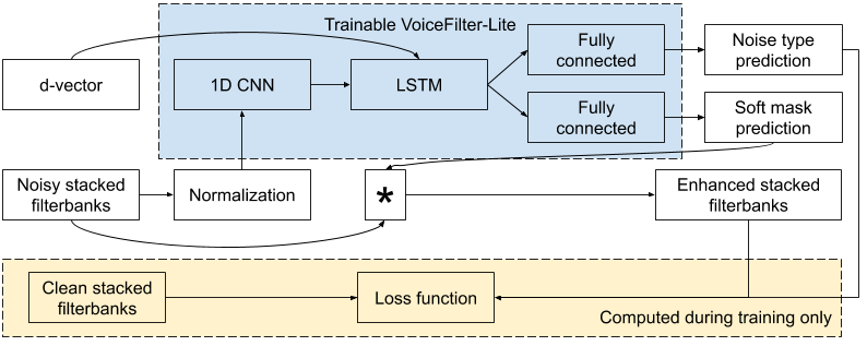
To train the VoiceFilter-Lite model, the filterbanks of the noisy speech are fed as input to the network together with an embedding vector that represents the identity of the target speaker (i.e., a d-vector). The network predicts a mask that is element-wise multiplied to the input to produce enhanced filterbanks. A loss function is defined to minimize the difference between the enhanced filterbanks and the filterbanks from the clean speech during training.

Model architecture of the VoiceFilter-Lite system.

VoiceFilter-Lite is a plug-and-play model, which allows the application in which it’s implemented to easily bypass it if the speaker did not enroll their voice. This also means that the speech recognition model and the VoiceFilter-Lite model can be separately trained and updated, which largely reduces engineering complexity in the deployment process.

As a plug-and-play model, VoiceFilter-Lite can be easily bypassed if the speaker did not enroll their voice.

Addressing the Challenge of Over-Suppression
When speech separation models are used for improving speech recognition, two types of error could occur: under-suppression, when the model fails to filter out noisy components from the signal; and over-suppression, when the model fails to preserve useful signal, resulting in some words being dropped from the recognized text. Over-suppression is especially problematic since modern speech recognition models are usually already trained with extensively augmented data (such as room simulation and SpecAugment), and thus are more robust to under-suppression.

VoiceFilter-Lite addresses the over-suppression issue with two novel approaches. First, it uses an asymmetric loss during the training process, such that the model is less tolerant to over-suppression than under-suppression. Second, it predicts the type of noise at runtime, and adaptively adjusts the suppression strength according to this prediction.

VoiceFilter-Lite adaptively applies stronger suppression strength when overlapping speech is detected.

With these two solutions, the VoiceFilter-Lite model retains great performance on streaming speech recognition for other scenarios, such as single-speaker speech under quiet or various noise conditions, while still providing significant improvement on overlapping speech. From our experiments, we observed a 25.1% improvement of word error rate after the 2.2MB VoiceFilter-Lite model is applied on additive overlapping speech. For reverberant overlapping speech, which is a more challenging task to simulate far-field devices such as smart home speakers, we also observed a 14.7% improvement of word error rate with VoiceFilter-Lite.

Future Work
While VoiceFilter-Lite has shown great promise for various on-device speech applications, we are also exploring several other directions to make VoiceFilter-Lite more useful. First, our current model is trained and evaluated with English speech only. We are excited about adopting the same technology to improve speech recognition for more languages. Second, we would like to directly optimize the speech recognition loss during the training of VoiceFilter-Lite, which can potentially further improve speech recognition beyond overlapping speech.

Acknowledgements
The research described in this post represents joint efforts from multiple teams within Google. Contributors include Quan Wang, Ignacio Lopez Moreno, Mert Saglam, Kevin Wilson, Alan Chiao, Renjie Liu, Yanzhang He, Wei Li, Jason Pelecanos, Philip Chao, Sinan Akay, John Han, Stephen Wu, Hannah Muckenhirn, Ye Jia, Zelin Wu, Yiteng Huang, Marily Nika, Jaclyn Konzelmann, Nino Tasca, and Alexander Gruenstein.

Source: Google AI Blog


Announcing the Objectron Dataset

The state of the art in machine learning (ML) has achieved exceptional accuracy on many computer vision tasks solely by training models on photos. Building upon these successes and advancing 3D object understanding has great potential to power a wider range of applications, such as augmented reality, robotics, autonomy, and image retrieval. For example, earlier this year we released MediaPipe Objectron, a set of real-time 3D object detection models designed for mobile devices, which were trained on a fully annotated, real-world 3D dataset, that can predict objects’ 3D bounding boxes.

Yet, understanding objects in 3D remains a challenging task due to the lack of large real-world datasets compared to 2D tasks (e.g., ImageNet, COCO, and Open Images). To empower the research community for continued advancement in 3D object understanding, there is a strong need for the release of object-centric video datasets, which capture more of the 3D structure of an object, while matching the data format used for many vision tasks (i.e., video or camera streams), to aid in the training and benchmarking of machine learning models.

Today, we are excited to release the Objectron dataset, a collection of short, object-centric video clips capturing a larger set of common objects from different angles. Each video clip is accompanied by AR session metadata that includes camera poses and sparse point-clouds. The data also contain manually annotated 3D bounding boxes for each object, which describe the object’s position, orientation, and dimensions. The dataset consists of 15K annotated video clips supplemented with over 4M annotated images collected from a geo-diverse sample (covering 10 countries across five continents).

Example videos in the Objectron dataset.

A 3D Object Detection Solution
Along with the dataset, we are also sharing a 3D object detection solution for four categories of objects — shoes, chairs, mugs, and cameras. These models are released in MediaPipe, Google's open source framework for cross-platform customizable ML solutions for live and streaming media, which also powers ML solutions like on-device real-time hand, iris and body pose tracking.

Sample results of 3D object detection solution running on mobile.

In contrast to the previously released single-stage Objectron model, these newest versions utilize a two-stage architecture. The first stage employs the TensorFlow Object Detection model to find the 2D crop of the object. The second stage then uses the image crop to estimate the 3D bounding box while simultaneously computing the 2D crop of the object for the next frame, so that the object detector does not need to run every frame. The second stage 3D bounding box predictor runs at 83 FPS on Adreno 650 mobile GPU.

Diagram of a reference 3D object detection solution.

Evaluation Metric for 3D Object Detection
With ground truth annotations, we evaluate the performance of 3D object detection models using 3D intersection over union (IoU) similarity statistics, a commonly used metric for computer vision tasks, which measures how close the bounding boxes are to the ground truth.

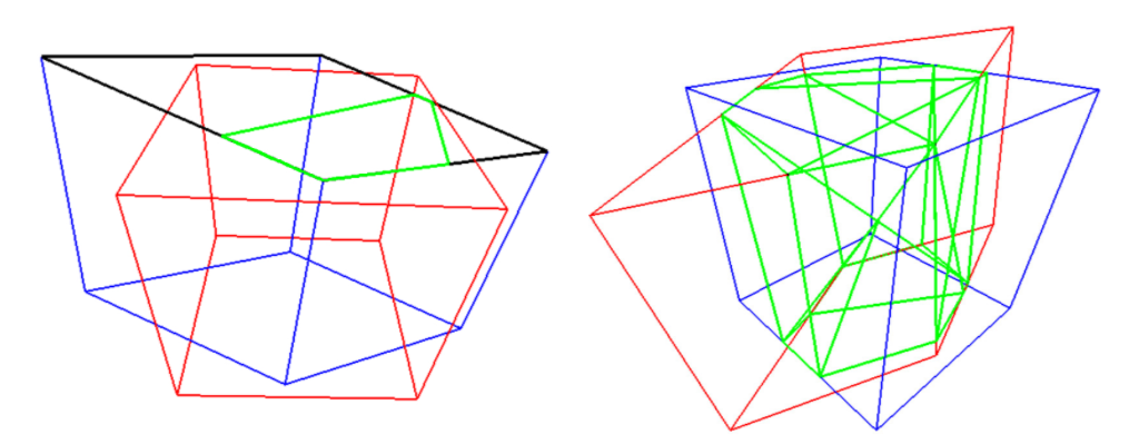
We propose an algorithm for computing accurate 3D IoU values for general 3D-oriented boxes. First, we compute the intersection points between faces of the two boxes using Sutherland-Hodgman Polygon clipping algorithm. This is similar to frustum culling, a technique used in computer graphics. The volume of the intersection is computed by the convex hull of all the clipped polygons. Finally, the IoU is computed from the volume of the intersection and volume of the union of two boxes. We are releasing the evaluation metrics source code along with the dataset.

Compute the 3D intersection over union using the polygon clipping algorithm, Left: Compute the intersection points of each face by clipping the polygon against the box. Right: Compute the volume of intersection by computing the convex hull of all intersection points (green).

Dataset Format
The technical details of the Objectron dataset, including usage and tutorials, are available on the dataset website. The dataset includes bikes, books, bottles, cameras, cereal boxes, chairs, cups, laptops, and shoes, and is stored in the objectron bucket on Google Cloud storage with the following assets:

  • The video sequences
  • The annotation labels (3D bounding boxes for objects)
  • AR metadata (such as camera poses, point clouds, and planar surfaces)
  • Processed dataset: shuffled version of the annotated frames, in tf.example format for images and SequenceExample format for videos.
  • Supporting scripts to run evaluation based on the metric described above
  • Supporting scripts to load the data into Tensorflow, PyTorch, and Jax and to visualize the dataset, including “Hello World” examples

With the dataset, we are also open-sourcing a data-pipeline to parse the dataset in popular Tensorflow, PyTorch and Jax frameworks. Example colab notebooks are also provided.

By releasing this Objectron dataset, we hope to enable the research community to push the limits of 3D object geometry understanding. We also hope to foster new research and applications, such as view synthesis, improved 3D representation, and unsupervised learning. Stay tuned for future activities and developments by joining our mailing list and visiting our github page.

Acknowledgements
The research described in this post was done by Adel Ahmadyan, Liangkai Zhang, Jianing Wei, Artsiom Ablavatski, Mogan Shieh, Ryan Hickman, Buck Bourdon, Alexander Kanaukou, Chuo-Ling Chang, Matthias Grundmann, ‎and Tom Funkhouser. We thank Aliaksandr Shyrokau, Sviatlana Mialik, Anna Eliseeva, and the annotation team for their high quality annotations. We also would like to thank Jonathan Huang and Vivek Rathod for their guidance on TensorFlow Object Detection API.

Source: Google AI Blog


Background Features in Google Meet, Powered by Web ML

Video conferencing is becoming ever more critical in people's work and personal lives. Improving that experience with privacy enhancements or fun visual touches can help center our focus on the meeting itself. As part of this goal, we recently announced ways to blur and replace your background in Google Meet, which use machine learning (ML) to better highlight participants regardless of their surroundings. Whereas other solutions require installing additional software, Meet’s features are powered by cutting-edge web ML technologies built with MediaPipe that work directly in your browser — no extra steps necessary. One key goal in developing these features was to provide real-time, in-browser performance on almost all modern devices, which we accomplished by combining efficient on-device ML models, WebGL-based rendering, and web-based ML inference via XNNPACK and TFLite.

Background blur and background replacement, powered by MediaPipe on the web.

Overview of Our Web ML Solution
The new features in Meet are developed with MediaPipe, Google's open source framework for cross-platform customizable ML solutions for live and streaming media, which also powers ML solutions like on-device real-time hand, iris and body pose tracking.

A core need for any on-device solution is to achieve high performance. To accomplish this, MediaPipe’s web pipeline leverages WebAssembly, a low-level binary code format designed specifically for web browsers that improves speed for compute-heavy tasks. At runtime, the browser converts WebAssembly instructions into native machine code that executes much faster than traditional JavaScript code. In addition, Chrome 84 recently introduced support for WebAssembly SIMD, which processes multiple data points with each instruction, resulting in a performance boost of more than 2x.

Our solution first processes each video frame by segmenting a user from their background (more about our segmentation model later in the post) utilizing ML inference to compute a low resolution mask. Optionally, we further refine the mask to align it with the image boundaries. The mask is then used to render the video output via WebGL2, with the background blurred or replaced.

WebML Pipeline: All compute-heavy operations are implemented in C++/OpenGL and run within the browser via WebAssembly.

In the current version, model inference is executed on the client’s CPU for low power consumption and widest device coverage. To achieve real-time performance, we designed efficient ML models with inference accelerated by the XNNPACK library, the first inference engine specifically designed for the novel WebAssembly SIMD specification. Accelerated by XNNPACK and SIMD, the segmentation model can run in real-time on the web.

Enabled by MediaPipe's flexible configuration, the background blur/replace solution adapts its processing based on device capability. On high-end devices it runs the full pipeline to deliver the highest visual quality, whereas on low-end devices it continues to perform at speed by switching to compute-light ML models and bypassing the mask refinement.

Segmentation Model
On-device ML models need to be ultra lightweight for fast inference, low power consumption, and small download size. For models running in the browser, the input resolution greatly affects the number of floating-point operations (FLOPs) necessary to process each frame, and therefore needs to be small as well. We downsample the image to a smaller size before feeding it to the model. Recovering a segmentation mask as fine as possible from a low-resolution image adds to the challenges of model design.

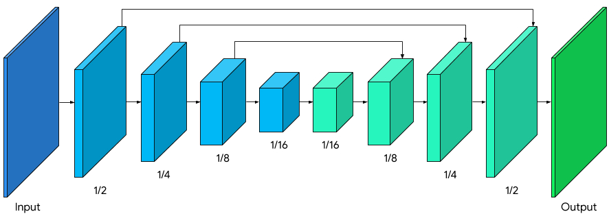
The overall segmentation network has a symmetric structure with respect to encoding and decoding, while the decoder blocks (light green) also share a symmetric layer structure with the encoder blocks (light blue). Specifically, channel-wise attention with global average pooling is applied in both encoder and decoder blocks, which is friendly to efficient CPU inference.

Model architecture with MobileNetV3 encoder (light blue), and a symmetric decoder (light green).

We modified MobileNetV3-small as the encoder, which has been tuned by network architecture search for the best performance with low resource requirements. To reduce the model size by 50%, we exported our model to TFLite using float16 quantization, resulting in a slight loss in weight precision but with no noticeable effect on quality. The resulting model has 193K parameters and is only 400KB in size.

Rendering Effects
Once segmentation is complete, we use OpenGL shaders for video processing and effect rendering, where the challenge is to render efficiently without introducing artifacts. In the refinement stage, we apply a joint bilateral filter to smooth the low resolution mask.

Rendering effects with artifacts reduced. Left: Joint bilateral filter smooths the segmentation mask. Middle: Separable filters remove halo artifacts in background blur. Right: Light wrapping in background replace.

The blur shader simulates a bokeh effect by adjusting the blur strength at each pixel proportionally to the segmentation mask values, similar to the circle-of-confusion (CoC) in optics. Pixels are weighted by their CoC radii, so that foreground pixels will not bleed into the background. We implemented separable filters for the weighted blur, instead of the popular Gaussian pyramid, as it removes halo artifacts surrounding the person. The blur is performed at a low resolution for efficiency, and blended with the input frame at the original resolution.

Background blur examples.

For background replacement, we adopt a compositing technique, known as light wrapping, for blending segmented persons and customized background images. Light wrapping helps soften segmentation edges by allowing background light to spill over onto foreground elements, making the compositing more immersive. It also helps minimize halo artifacts when there is a large contrast between the foreground and the replaced background.

Background replacement examples.

Performance
To optimize the experience for different devices, we provide model variants at multiple input sizes (i.e., 256x144 and 160x96 in the current release), automatically selecting the best according to available hardware resources.

We evaluated the speed of model inference and the end-to-end pipeline on two common devices: MacBook Pro 2018 with 2.2 GHz 6-Core Intel Core i7, and Acer Chromebook 11 with Intel Celeron N3060. For 720p input, the MacBook Pro can run the higher-quality model at 120 FPS and the end-to-end pipeline at 70 FPS, while the Chromebook runs inference at 62 FPS with the lower-quality model and 33 FPS end-to-end.

 Model   FLOPs   Device   Model Inference   Pipeline 
 256x144   64M   MacBook Pro 18   8.3ms (120 FPS)   14.3ms (70 FPS) 
 160x96   27M   Acer Chromebook 11   16.1ms (62 FPS)   30ms (33 FPS) 
Model inference speed and end-to-end pipeline on high-end (MacBook Pro) and low-end (Chromebook) laptops.

For quantitative evaluation of model accuracy, we adopt the popular metrics of intersection-over-union (IOU) and boundary F-measure. Both models achieve high quality, especially for having such a lightweight network:

  Model     IOU     Boundary  
  F-measure  
  256x144     93.58%     0.9024  
  160x96     90.79%     0.8542  
Evaluation of model accuracy, measured by IOU and boundary F-score.

We also release the accompanying Model Card for our segmentation models, which details our fairness evaluations. Our evaluation data contains images from 17 geographical subregions of the globe, with annotations for skin tone and gender. Our analysis shows that the model is consistent in its performance across the various regions, skin-tones, and genders, with only small deviations in IOU metrics.

Conclusion
We introduced a new in-browser ML solution for blurring and replacing your background in Google Meet. With this, ML models and OpenGL shaders can run efficiently on the web. The developed features achieve real-time performance with low power consumption, even on low-power devices.

Acknowledgments
Special thanks to those on the Meet team and others who worked on this project, in particular Sebastian Jansson, Rikard Lundmark, Stephan Reiter, Fabian Bergmark, Ben Wagner, Stefan Holmer, Dan Gunnarson, Stéphane Hulaud and to all our team members who worked on the technology with us: Siargey Pisarchyk, Karthik Raveendran, Chris McClanahan, Marat Dukhan, Frank Barchard, Ming Guang Yong, Chuo-Ling Chang, Michael Hays, Camillo Lugaresi, Gregory Karpiak, Siarhei Kazakou, Matsvei Zhdanovich, and Matthias Grundmann.

Source: Google AI Blog