Author Archives: Google AI

Google at ICML 2021

Groups across Google are actively pursuing research across the field of machine learning, ranging from theory to application. With scalable tools and architectures, we build machine learning systems to solve deep scientific and engineering challenges in areas of language, music, visual processing, and more.

Google is proud to be a Platinum Sponsor of the thirty-eighth International Conference on Machine Learning (ICML 2021), a premier annual event happening this week. As a leader in machine learning research — with over 100 accepted publications and Googlers participating in workshops — we look forward to our continued partnership with the broader machine learning research community.

Registered for ICML 2021? We hope you’ll visit the Google virtual booth to learn more about the exciting work, creativity, and fun that goes into solving a portion of the field’s most interesting challenges. Take a look below to learn more about the Google research being presented at ICML 2021 (Google affiliations in bold).

Organizing Committee
ICML Board Members include: Corinna Cortes, Hugo Larochelle, Shakir Mohamed
ICML Emeritus Board includes: William Cohen, Andrew McCallum
Tutorial Co-Chair member: Quoc Lee

Publications
Attention Is Not All You Need: Pure Attention Loses Rank Doubly Exponentially with Depth
Yihe Dong, Jean-Baptiste Cordonnier, Andreas Loukas

Scalable Evaluation of Multi-agent Reinforcement Learning with Melting Pot
Joel Z. Leibo, Edgar Duéñez-Guzmán, Alexander Sasha Vezhnevets, John P. Agapiou, Peter Sunehag, Raphael Koster, Jayd Matyas, Charles Beattie, Igor Mordatch, Thore Graepel

On the Optimality of Batch Policy Optimization Algorithms
Chenjun Xiao, Yifan Wu, Tor Lattimore, Bo Dai, Jincheng Mei, Lihong Li*, Csaba Szepesvari, Dale Schuurmans

Low-Rank Sinkhorn Factorization
Meyer Scetbon, Marco Cuturi, Gabriel Peyré

Oops I Took A Gradient: Scalable Sampling for Discrete Distributions
Will Grathwohl, Kevin Swersky, Milad Hashemi, David Duvenaud, Chris J. Maddison

PID Accelerated Value Iteration Algorithm
Amir-Massoud Farahmand, Mohammad Ghavamzadeh

Dueling Convex Optimization
Aadirupa Saha, Tomer Koren, Yishay Mansour

What Are Bayesian Neural Network Posteriors Really Like?
Pavel Izmailov, Sharad Vikram, Matthew D. Hoffman, Andrew Gordon Wilson

Offline Reinforcement Learning with Pseudometric Learning
Robert Dadashi, Shideh Rezaeifar, Nino Vieillard, Léonard Hussenot, Olivier Pietquin, Matthieu Geist

Revisiting Rainbow: Promoting More Insightful and Inclusive Deep Reinforcement Learning Research (see blog post)
Johan S. Obando-Ceron, Pablo Samuel Castro

EMaQ: Expected-Max Q-Learning Operator for Simple Yet Effective Offline and Online RL
Seyed Kamyar Seyed Ghasemipour*, Dale Schuurmans, Shixiang Shane Gu

Variational Data Assimilation with a Learned Inverse Observation Operator
Thomas Frerix, Dmitrii Kochkov, Jamie A. Smith, Daniel Cremers, Michael P. Brenner, Stephan Hoyer

Tilting the Playing Field: Dynamical Loss Functions for Machine Learning
Miguel Ruiz-Garcia, Ge Zhang, Samuel S. Schoenholz, Andrea J. Liu

Model-Based Reinforcement Learning via Latent-Space Collocation
Oleh Rybkin, Chuning Zhu, Anusha Nagabandi, Kostas Daniilidis, Igor Mordatch, Sergey Levine

Momentum Residual Neural Networks
Michael E. Sander, Pierre Ablin, Mathieu Blondel, Gabriel Peyré

OmniNet: Omnidirectional Representations from Transformers
Yi Tay, Mostafa Dehghani, Vamsi Aribandi, Jai Gupta, Philip Pham, Zhen Qin, Dara Bahri, Da-Cheng Juan, Donald Metzler

Synthesizer: Rethinking Self-Attention for Transformer Models
Yi Tay, Dara Bahri, Donald Metzler, Da-Cheng Juan, Zhe Zhao, Che Zheng

Towards Domain-Agnostic Contrastive Learning
Vikas Verma, Minh-Thang Luong, Kenji Kawaguchi, Hieu Pham, Quoc V. Le

Randomized Entity-wise Factorization for Multi-agent Reinforcement Learning
Shariq Iqbal, Christian A. Schroeder de Witt, Bei Peng, Wendelin Böhmer, Shimon Whiteson, Fei Sha

LIME: Learning Inductive Bias for Primitives of Mathematical Reasoning
Yuhuai Wu, Markus Rabe, Wenda Li, Jimmy Ba, Roger Grosse, Christian Szegedy

Emergent Social Learning via Multi-agent Reinforcement Learning
Kamal Ndousse, Douglas Eck, Sergey Levine, Natasha Jaques

Improved Contrastive Divergence Training of Energy-Based Models
Yilun Du, Shuang Li, Joshua Tenenbaum, Igor Mordatch

Characterizing Structural Regularities of Labeled Data in Overparameterized Models
Ziheng Jiang*, Chiyuan Zhang, Kunal Talwar, Michael Mozer

Actionable Models: Unsupervised Offline Reinforcement Learning of Robotic Skills
Yevgen Chebotar, Karol Hausman, Yao Lu, Ted Xiao, Dmitry Kalashnikov, Jake Varley, Alex Irpan, Benjamin Eysenbach, Ryan Julian, Chelsea Finn, Sergey Levine

PsiPhi-Learning: Reinforcement Learning with Demonstrations using Successor Features and Inverse Temporal Difference Learning
Angelos Filos, Clare Lyle, Yarin Gal, Sergey Levine, Natasha Jaques, Gregory Farquhar

EfficientNetV2: Smaller Models and Faster Training
Mingxing Tan, Quoc V. Le

Unbiased Gradient Estimation in Unrolled Computation Graphs with Persistent Evolution Strategies
Paul Vicol, Luke Metz, Jascha Sohl-Dickstein

Federated Composite Optimization
Honglin Yuan*, Manzil Zaheer, Sashank Reddi

Light RUMs
Flavio Chierichetti, Ravi Kumar, Andrew Tomkins

Catformer: Designing Stable Transformers via Sensitivity Analysis
Jared Quincy Davis, Albert Gu, Krzysztof Choromanski, Tri Dao, Christopher Re, Chelsea Finn, Percy Liang

Representation Matters: Offline Pretraining for Sequential Decision Making
Mengjiao Yang, Ofir Nachum

Variational Empowerment as Representation Learning for Goal-Conditioned Reinforcement Learning
Jongwook Choi*, Archit Sharma*, Honglak Lee, Sergey Levine, Shixiang Shane Gu

Beyond Variance Reduction: Understanding the True Impact of Baselines on Policy Optimization
Wesley Chung, Valentin Thomas, Marlos C. Machado, Nicolas Le Roux

Whitening and Second Order Optimization Both Make Information in the Dataset Unusable During Training, and Can Reduce or Prevent Generalization
Neha S. Wadia, Daniel Duckworth, Samuel S. Schoenholz, Ethan Dyer, Jascha Sohl-Dickstein

Understanding Invariance via Feedforward Inversion of Discriminatively Trained Classifiers
Piotr Teterwak*, Chiyuan Zhang, Dilip Krishnan, Michael C. Mozer

Policy Information Capacity: Information-Theoretic Measure for Task Complexity in Deep Reinforcement Learning
Hiroki Furuta, Tatsuya Matsushima, Tadashi Kozuno, Yutaka Matsuo, Sergey Levine, Ofir Nachum, Shixiang Shane Gu

Hyperparameter Selection for Imitation Learning
Leonard Hussenot, Marcin Andrychowicz, Damien Vincent, Robert Dadashi, Anton Raichuk, Lukasz Stafiniak, Sertan Girgin, Raphael Marinier, Nikola Momchev, Sabela Ramos, Manu Orsini, Olivier Bachem, Matthieu Geist, Olivier Pietquin

Disentangling Sampling and Labeling Bias for Learning in Large-Output Spaces
Ankit Singh Rawat, Aditya Krishna Menon, Wittawat Jitkrittum, Sadeep Jayasumana, Felix X. Yu, Sashank J. Reddi, Sanjiv Kumar

Revenue-Incentive Tradeoffs in Dynamic Reserve Pricing
Yuan Deng, Sebastien Lahaie, Vahab Mirrokni, Song Zuo

Debiasing a First-Order Heuristic for Approximate Bi-Level Optimization
Valerii Likhosherstov, Xingyou Song, Krzysztof Choromanski, Jared Davis, Adrian Weller

Characterizing the Gap Between Actor-Critic and Policy Gradient
Junfeng Wen, Saurabh Kumar, Ramki Gummadi, Dale Schuurmans

Composing Normalizing Flows for Inverse Problems
Jay Whang, Erik Lindgren, Alexandros Dimakis

Online Policy Gradient for Model Free Learning of Linear Quadratic Regulators with √T Regret
Asaf Cassel, Tomer Koren

Learning to Price Against a Moving Target
Renato Paes Leme, Balasubramanian Sivan, Yifeng Teng, Pratik Worah

Fairness and Bias in Online Selection
Jose Correa, Andres Cristi, Paul Duetting, Ashkan Norouzi-Fard

The Impact of Record Linkage on Learning from Feature Partitioned Data
Richard Nock, Stephen Hardy, Wilko Henecka, Hamish Ivey-Law, Jakub Nabaglo, Giorgio Patrini, Guillaume Smith, Brian Thorne

Reserve Price Optimization for First Price Auctions in Display Advertising
Zhe Feng*, Sébastien Lahaie, Jon Schneider, Jinchao Ye

A Regret Minimization Approach to Iterative Learning Control
Naman Agarwal, Elad Hazan, Anirudha Majumdar, Karan Singh

A Statistical Perspective on Distillation
Aditya Krishna Menon, Ankit Singh Rawat, Sashank J. Reddi, Seungyeon Kim, Sanjiv Kumar

Best Model Identification: A Rested Bandit Formulation
Leonardo Cella, Massimiliano Pontil, Claudio Gentile

Generalised Lipschitz Regularisation Equals Distributional Robustness
Zac Cranko, Zhan Shi, Xinhua Zhang, Richard Nock, Simon Kornblith

Stochastic Multi-armed Bandits with Unrestricted Delay Distributions
Tal Lancewicki, Shahar Segal, Tomer Koren, Yishay Mansour

Regularized Online Allocation Problems: Fairness and Beyond
Santiago Balseiro, Haihao Lu, Vahab Mirrokni

Implicit Rate-Constrained Optimization of Non-decomposable Objectives
Abhishek Kumar, Harikrishna Narasimhan, Andrew Cotter

Leveraging Non-uniformity in First-Order Non-Convex Optimization
Jincheng Mei, Yue Gao, Bo Dai, Csaba Szepesvari, Dale Schuurmans

Dynamic Balancing for Model Selection in Bandits and RL
Ashok Cutkosky, Christoph Dann, Abhimanyu Das, Claudio Gentile, Aldo Pacchiano, Manish Purohit

Adversarial Dueling Bandits
Aadirupa Saha, Tomer Koren, Yishay Mansour

Optimizing Black-Box Metrics with Iterative Example Weighting
Gaurush Hiranandani*, Jatin Mathur, Harikrishna Narasimhan, Mahdi Milani Fard, Oluwasanmi Koyejo

Relative Deviation Margin Bounds
Corinna Cortes, Mehryar Mohri, Ananda Theertha Suresh

MC-LSTM: Mass-Conserving LSTM
Pieter-Jan Hoedt, Frederik Kratzert, Daniel Klotz, Christina Halmich, Markus Holzleitner, Grey Nearing, Sepp Hochreiter, Günter Klambauer

12-Lead ECG Reconstruction via Koopman Operators
Authors:Tomer Golany, Kira Radinsky, Daniel Freedman, Saar Minha

Finding Relevant Information via a Discrete Fourier Expansion
Mohsen Heidari, Jithin Sreedharan, Gil Shamir, Wojciech Szpankowski

LEGO: Latent Execution-Guided Reasoning for Multi-hop Question Answering on Knowledge Graphs
Hongyu Ren, Hanjun Dai, Bo Dai, Xinyun Chen, Michihiro Yasunaga, Haitian Sun, Dale Schuurmans, Jure Leskovec, Denny Zhou

SpreadsheetCoder: Formula Prediction from Semi-structured Context
Xinyun Chen, Petros Maniatis, Rishabh Singh, Charles Sutton, Hanjun Dai, Max Lin, Denny Zhou

Combinatorial Blocking Bandits with Stochastic Delays
Alexia Atsidakou, Orestis Papadigenopoulos, Soumya Basu, Constantine Caramani, Sanjay Shakkottai

Beyond log2(T) Regret for Decentralized Bandits in Matching Markets
Soumya Basu, Karthik Abinav Sankararaman, Abishek Sankararaman

Robust Pure Exploration in Linear Bandits with Limited Budget
Ayya Alieva, Ashok Cutkosky, Abhimanyu Das

Latent Programmer: Discrete Latent Codes for Program Synthesis
Joey Hong, David Dohan, Rishabh Singh, Charles Sutton, Manzil Zaheer

Scaling Up Visual and Vision-Language Representation Learning With Noisy Text Supervision (see blog post)
Chao Jia, Yinfei Yang, Ye Xia, Yi-Ting Chen, Zarana Parekh, Hieu Pham, Quoc V. Le, Yunhsuan Sung, Zhen Li, Tom Duerig

On Linear Identifiability of Learned Representations
Geoffrey Roeder, Luke Metz, Diederik P. Kingma

Hierarchical Clustering of Data Streams: Scalable Algorithms and Approximation Guarantees
Anand Rajagopalan, Fabio Vitale, Danny Vainstein, Gui Citovsky, Cecilia M Procopiuc, Claudio Gentile

Differentially Private Quantiles
Jennifer Gillenwater, Matthew Joseph, Alex Kulesza

Active Covering
Heinrich Jiang, Afshin Rostamizadeh

Sharf: Shape-Conditioned Radiance Fields from a Single View
Konstantinos Rematas, Ricardo Martin-Brualla, Vittorio Ferrari

Learning a Universal Template for Few-Shot Dataset Generalization
Eleni Triantafillou*, Hugo Larochelle, Richard Zemel, Vincent Dumoulin

Private Alternating Least Squares: Practical Private Matrix Completion with Tighter Rates
Steve Chien, Prateek Jain, Walid Krichene, Steffen Rendle, Shuang Song, Abhradeep Thakurta, Li Zhang

Differentially-Private Clustering of Easy Instances
Edith Cohen, Haim Kaplan, Yishay Mansour, Uri Stemmer, Eliad Tsfadia

Label-Only Membership Inference Attacks
Christopher A. Choquette-Choo, Florian Tramèr, Nicholas Carlini, Nicolas Papernot

Neural Feature Matching in Implicit 3D Representations
Yunlu Chen, Basura Fernando, Hakan Bilen, Thomas Mensink, Efstratios Gavves

Locally Private k-Means in One Round
Alisa Chang, Badih Ghazi, Ravi Kumar, Pasin Manurangsi

Large-Scale Meta-learning with Continual Trajectory Shifting
Jaewoong Shin, Hae Beom Lee, Boqing Gong, Sung Ju Hwang

Statistical Estimation from Dependent Data
Vardis Kandiros, Yuval Dagan, Nishanth Dikkala, Surbhi Goel, Constantinos Daskalakis

Oneshot Differentially Private Top-k Selection
Gang Qiao, Weijie J. Su, Li Zhang

Unsupervised Part Representation by Flow Capsules
Sara Sabour, Andrea Tagliasacchi, Soroosh Yazdani, Geoffrey E. Hinton, David J. Fleet

Private Stochastic Convex Optimization: Optimal Rates in L1 Geometry
Hilal Asi, Vitaly Feldman, Tomer Koren, Kunal Talwar

Practical and Private (Deep) Learning Without Sampling or Shuffling
Peter Kairouz, Brendan McMahan, Shuang Song, Om Thakkar, Abhradeep Thakurta, Zheng Xu

Differentially Private Aggregation in the Shuffle Model: Almost Central Accuracy in Almost a Single Message
Badih Ghazi, Ravi Kumar, Pasin Manurangsi, Rasmus Pagh, Amer Sinha

Leveraging Public Data for Practical Private Query Release
Terrance Liu, Giuseppe Vietri, Thomas Steinke, Jonathan Ullman, Zhiwei Steven Wu

Meta-Thompson Sampling
Branislav Kveton, Mikhail Konobeev, Manzil Zaheer, Chih-wei Hsu, Martin Mladenov, Craig Boutilier, Csaba Szepesvári

Implicit-PDF: Non-parametric Representation of Probability Distributions on the Rotation Manifold
Kieran A Murphy, Carlos Esteves, Varun Jampani, Srikumar Ramalingam, Ameesh Makadia

Improving Ultrametrics Embeddings Through Coresets
Vincent Cohen-Addad, Rémi de Joannis de Verclos, Guillaume Lagarde

A Discriminative Technique for Multiple-Source Adaptation
Corinna Cortes, Mehryar Mohri, Ananda Theertha Suresh, Ningshan Zhang

Self-Supervised and Supervised Joint Training for Resource-Rich Machine Translation
Yong Cheng, Wei Wang*, Lu Jiang, Wolfgang Macherey

Correlation Clustering in Constant Many Parallel Rounds
Vincent Cohen-Addad, Silvio Lattanzi, Slobodan Mitrović, Ashkan Norouzi-Fard, Nikos Parotsidis, Jakub Tarnawski

Hierarchical Agglomerative Graph Clustering in Nearly-Linear Time
Laxman Dhulipala, David Eisenstat, Jakub Łącki, Vahab Mirrokni, Jessica Shi

Meta-learning Bidirectional Update Rules
Mark Sandler, Max Vladymyrov, Andrey Zhmoginov, Nolan Miller, Andrew Jackson, Tom Madams, Blaise Aguera y Arcas

Discretization Drift in Two-Player Games
Mihaela Rosca, Yan Wu, Benoit Dherin, David G.T. Barrett

Reasoning Over Virtual Knowledge Bases With Open Predicate Relations
Haitian Sun*, Pat Verga, Bhuwan Dhingra, Ruslan Salakhutdinov, William W. Cohen

Learn2Hop: Learned Optimization on Rough Landscapes
Amil Merchant, Luke Metz, Samuel Schoenholz, Ekin Cubuk

Locally Adaptive Label Smoothing Improves Predictive Churn
Dara Bahri, Heinrich Jiang

Overcoming Catastrophic Forgetting by Bayesian Generative Regularization
Patrick H. Chen, Wei Wei, Cho-jui Hsieh, Bo Dai

Workshops (only Google affiliations are noted)
LatinX in AI (LXAI) Research at ICML 2021
Hosts: Been Kim, Natasha Jaques

Uncertainty and Robustness in Deep Learning
Organizers: Balaji Lakshminarayanan, Jasper Snoek Invited Speaker: Dustin Tran

Reinforcement Learning for Real Life
Organizers: Minmin Chen, Lihong Li Invited Speaker: Ed Chi

Interpretable Machine Learning in Healthcare
Organizers: Alan Karthikesalingam Invited Speakers: Abhijit Guha Roy, Jim Winkens

The Neglected Assumptions in Causal Inference
Organizer: Alexander D'Amour

ICML Workshop on Algorithmic Recourse
Invited Speakers: Been Kim, Berk Ustun

A Blessing in Disguise: The Prospects and Perils of Adversarial Machine Learning
Invited Speaker: Nicholas Carlini

Overparameterization: Pitfalls and Opportunities
Organizers: Yasaman Bahri, Hanie Sedghi

Information-Theoretic Methods for Rigorous, Responsible, and Reliable Machine Learning (ITR3)
Invited Speaker: Thomas Steinke

Beyond First-Order Methods in Machine Learning Systems
Invited Speaker: Courtney Paquette

ICML 2021 Workshop: Self-Supervised Learning for Reasoning and Perception
Invited Speaker: Chelsea Finn

Workshop on Reinforcement Learning Theory
Invited Speaker: Bo Dai

Tutorials (only Google affiliations are noted)
Responsible AI in Industry: Practical Challenges and Lessons Learned
Organizers: Ben Packer

Online and Non-stochastic Control
Organizers: Elad Hazan

Random Matrix Theory and ML (RMT +ML)
Organizers: Fabian Pedregosa, Jeffrey Pennington, Courntey Paquette Self-Attention for Computer Vision Organizers: Prajit Ramachandran, Ashish Vaswani

* Indicates work done while at Google

Source: Google AI Blog


High Fidelity Image Generation Using Diffusion Models

Natural image synthesis is a broad class of machine learning (ML) tasks with wide-ranging applications that pose a number of design challenges. One example is image super-resolution, in which a model is trained to transform a low resolution image into a detailed high resolution image (e.g., RAISR). Super-resolution has many applications that can range from restoring old family portraits to improving medical imaging systems. Another such image synthesis task is class-conditional image generation, in which a model is trained to generate a sample image from an input class label. The resulting generated sample images can be used to improve performance of downstream models for image classification, segmentation, and more.

Generally, these image synthesis tasks are performed by deep generative models, such as GANs, VAEs, and autoregressive models. Yet each of these generative models has its downsides when trained to synthesize high quality samples on difficult, high resolution datasets. For example, GANs often suffer from unstable training and mode collapse, and autoregressive models typically suffer from slow synthesis speed.

Alternatively, diffusion models, originally proposed in 2015, have seen a recent revival in interest due to their training stability and their promising sample quality results on image and audio generation. Thus, they offer potentially favorable trade-offs compared to other types of deep generative models. Diffusion models work by corrupting the training data by progressively adding Gaussian noise, slowly wiping out details in the data until it becomes pure noise, and then training a neural network to reverse this corruption process. Running this reversed corruption process synthesizes data from pure noise by gradually denoising it until a clean sample is produced. This synthesis procedure can be interpreted as an optimization algorithm that follows the gradient of the data density to produce likely samples.

Today we present two connected approaches that push the boundaries of the image synthesis quality for diffusion models — Super-Resolution via Repeated Refinements (SR3) and a model for class-conditioned synthesis, called Cascaded Diffusion Models (CDM). We show that by scaling up diffusion models and with carefully selected data augmentation techniques, we can outperform existing approaches. Specifically, SR3 attains strong image super-resolution results that surpass GANs in human evaluations. CDM generates high fidelity ImageNet samples that surpass BigGAN-deep and VQ-VAE2 on both FID score and Classification Accuracy Score by a large margin.

SR3: Image Super-Resolution
SR3 is a super-resolution diffusion model that takes as input a low-resolution image, and builds a corresponding high resolution image from pure noise. The model is trained on an image corruption process in which noise is progressively added to a high-resolution image until only pure noise remains. It then learns to reverse this process, beginning from pure noise and progressively removing noise to reach a target distribution through the guidance of the input low-resolution image..

With large scale training, SR3 achieves strong benchmark results on the super-resolution task for face and natural images when scaling to resolutions 4x–8x that of the input low-resolution image. These super-resolution models can further be cascaded together to increase the effective super-resolution scale factor, e.g., stacking a 64x64 → 256x256 and a 256x256 → 1024x1024 face super-resolution model together in order to perform a 64x64 → 1024x1024 super-resolution task.

We compare SR3 with existing methods using human evaluation study. We conduct a Two-Alternative Forced Choice Experiment where subjects are asked to choose between the reference high resolution image, and the model output when asked the question, “Which image would you guess is from a camera?” We measure the performance of the model through confusion rates (% of time raters choose the model outputs over reference images, where a perfect algorithm would achieve a 50% confusion rate). The results of this study are shown in the figure below.

Above: We achieve close to 50% confusion rate on the task of 16x16 → 128x128 faces, outperforming state-of-the-art face super-resolution methods PULSE and FSRGAN. Below: We also achieve a 40% confusion rate on the much more difficult task of 64x64 → 256x256 natural images, outperforming the regression baseline by a large margin.

CDM: Class-Conditional ImageNet Generation
Having shown the effectiveness of SR3 in performing natural image super-resolution, we go a step further and use these SR3 models for class-conditional image generation. CDM is a class-conditional diffusion model trained on ImageNet data to generate high-resolution natural images. Since ImageNet is a difficult, high-entropy dataset, we built CDM as a cascade of multiple diffusion models. This cascade approach involves chaining together multiple generative models over several spatial resolutions: one diffusion model that generates data at a low resolution, followed by a sequence of SR3 super-resolution diffusion models that gradually increase the resolution of the generated image to the highest resolution. It is well known that cascading improves quality and training speed for high resolution data, as shown by previous studies (for example in autoregressive models and VQ-VAE-2) and in concurrent work for diffusion models. As demonstrated by our quantitative results below, CDM further highlights the effectiveness of cascading in diffusion models for sample quality and usefulness in downstream tasks, such as image classification.

Example of the cascading pipeline that includes a sequence of diffusion models: the first generates a low resolution image, and the rest perform upsampling to the final high resolution image. Here the pipeline is for class-conditional ImageNet generation, which begins with a class-conditional diffusion model at 32x32 resolution, followed by 2x and 4x class-conditional super-resolution using SR3.
Selected generated images from our 256x256 cascaded class-conditional ImageNet model.

Along with including the SR3 model in the cascading pipeline, we also introduce a new data augmentation technique, which we call conditioning augmentation, that further improves the sample quality results of CDM. While the super-resolution models in CDM are trained on original images from the dataset, during generation they need to perform super-resolution on the images generated by a low-resolution base model, which may not be of sufficiently high quality in comparison to the original images. This leads to a train-test mismatch for the super-resolution models. Conditioning augmentation refers to applying data augmentation to the low-resolution input image of each super-resolution model in the cascading pipeline. These augmentations, which in our case include Gaussian noise and Gaussian blur, prevents each super-resolution model from overfitting to its lower resolution conditioning input, eventually leading to better higher resolution sample quality for CDM.

Altogether, CDM generates high fidelity samples superior to BigGAN-deep and VQ-VAE-2 in terms of both FID score and Classification Accuracy Score on class-conditional ImageNet generation. CDM is a pure generative model that does not use a classifier to boost sample quality, unlike other models such as ADM and VQ-VAE-2. See below for quantitative results on sample quality.

Class-conditional ImageNet FID scores at the 256x256 resolution for methods that do not use extra classifiers to boost sample quality. BigGAN-deep is reported at its best truncation value. (Lower is better.)
ImageNet classification accuracy scores at the 256x256 resolution, measuring the validation set accuracy of a classifier trained on generated data. CDM generated data attains significant gains over existing methods, closing the gap in classification accuracy between real and generated data. (Higher is better.)

Conclusion
With SR3 and CDM, we have pushed the performance of diffusion models to state-of-the-art on super-resolution and class-conditional ImageNet generation benchmarks. We are excited to further test the limits of diffusion models for a wide variety of generative modeling problems. For more information on our work, please visit Image Super-Resolution via Iterative Refinement and Cascaded Diffusion Models for High Fidelity Image Generation.

Acknowledgements:
We thank our co-authors William Chan, Mohammad Norouzi, Tim Salimans, and David Fleet, and we are grateful for research discussions and assistance from Ben Poole, Jascha Sohl-Dickstein, Doug Eck, and the rest of the Google Research, Brain Team. Thanks to Tom Small for helping us with the animations.

Source: Google AI Blog


Speeding Up Reinforcement Learning with a New Physics Simulation Engine

Reinforcement learning (RL) is a popular method for teaching robots to navigate and manipulate the physical world, which itself can be simplified and expressed as interactions between rigid bodies1 (i.e., solid physical objects that do not deform when a force is applied to them). In order to facilitate the collection of training data in a practical amount of time, RL usually leverages simulation, where approximations of any number of complex objects are composed of many rigid bodies connected by joints and powered by actuators. But this poses a challenge: it frequently takes millions to billions of simulation frames for an RL agent to become proficient at even simple tasks, such as walking, using tools, or assembling toy blocks.

While progress has been made to improve training efficiency by recycling simulation frames, some RL tools instead sidestep this problem by distributing the generation of simulation frames across many simulators. These distributed simulation platforms yield impressive results that train very quickly, but they must run on compute clusters with thousands of CPUs or GPUs which are inaccessible to most researchers.

In “Brax - A Differentiable Physics Engine for Large Scale Rigid Body Simulation”, we present a new physics simulation engine that matches the performance of a large compute cluster with just a single TPU or GPU. The engine is designed to both efficiently run thousands of parallel physics simulations alongside a machine learning (ML) algorithm on a single accelerator and scale millions of simulations seamlessly across pods of interconnected accelerators. We’ve open sourced the engine along with reference RL algorithms and simulation environments that are all accessible via Colab. Using this new platform, we demonstrate 100-1000x faster training compared to a traditional workstation setup.

Three typical RL workflows. The left shows a typical workstation flow: on a single machine, with the environment on CPU, training takes hours or days. The middle shows a typical distributed simulation flow: training takes minutes by farming simulation out to thousands of machines. The right shows the Brax flow: learning and large batch simulation occur side by side on a single CPU/GPU chip.

Physics Simulation Engine Design Opportunities
Rigid body physics are used in video games, robotics, molecular dynamics, biomechanics, graphics and animation, and other domains. In order to accurately model such systems, simulators integrate forces from gravity, motor actuation, joint constraints, object collisions, and others to simulate the motion of a physical system across time.

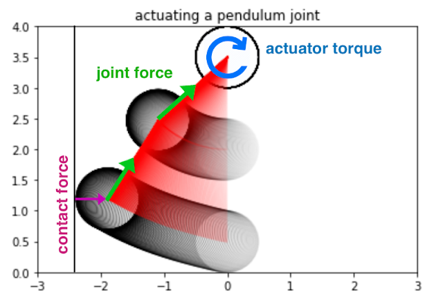
Simulation of three spherical bodies, a wall, two joints, and one actuator. For each simulation timestep, forces and torques are integrated together to update the positions, rotations, and velocities of each physical body.

Taking a closer look at how most physics simulation engines are designed today, there are a few large opportunities to improve efficiency. As we noted above, a typical robotics learning pipeline places a single learner in a tight feedback with many simulations in parallel, but upon analyzing this architecture, one finds that:

  1. This layout imposes an enormous latency bottleneck. Because the data must travel over the network within a datacenter, the learner must wait for 10,000+ nanoseconds to fetch experience from the simulator. Were this experience instead already on the same device as the learner’s neural network, latency would drop to <1 nanosecond.
  2. The computation necessary for training the agent (one simulation step, followed by one update of the agent’s neural network) is overshadowed by the computation spent packaging the data (i.e., marshalling data within the engine, then into a wire format such as protobuf, then into TCP buffers, and then undoing all these steps on the learner side).
  3. The computations happening within each simulator are remarkably similar, but not exactly the same.

Brax Design
In response to these observations, Brax is designed so that its physics calculations are exactly the same across each of its thousands of parallel environments by ensuring that the simulation is free of branches (i.e., simulation “if” logic that diverges as a result of the environment state). An example of a branch in a physics engine is the application of a contact force between a ball and a wall: different code paths will execute depending on whether the ball is touching the wall. That is, if the ball contacts the wall, separate code for simulating the ball’s bounce off the wall will execute. Brax employs a mix of the following three strategies to avoid branching:

  • Replace the discrete branching logic with a continuous function, such as approximating the ball-wall contact force using a signed distance function. This approach results in the most efficiency gains.
  • Evaluate the branch during JAX’s just-in-time compile. Many branches based on static properties of the environment, such as whether it’s even possible for two objects to collide, may be evaluated prior to simulation time.
  • Run both sides of the branch during simulation but then select only the required results. Because this executes some code that isn’t ultimately used, it wastes operations compared to the above.

Once the calculations are guaranteed to be exactly uniform, the entire training architecture can be reduced in complexity to be executed on a single TPU or GPU. Doing so removes the computational overhead and latency of cross-machine communication. In practice, these changes lower the cost of training by 100x-1000x for comparable workloads.

Brax Environments
Environments are tiny packaged worlds that define a task for an RL agent to learn. Environments contain not only the means to simulate a world, but also functions, such as how to observe the world and the definition of the goal in that world.

A few standard benchmark environments have emerged in recent years for testing new RL algorithms and for evaluating the impact of those algorithms using metrics commonly understood by research scientists. Brax includes four such ready-to-use environments that come from the popular OpenAI gym: Ant, HalfCheetah, Humanoid, and Reacher.


From left to right: Ant, HalfCheetah, Humanoid, and Reacher are popular baseline environments for RL research.

Brax also includes three novel environments: dexterous manipulation of an object (a popular challenge in robotics), generalized locomotion (an agent that goes to a target placed anywhere around it), and a simulation of an industrial robot arm.


Left: Grasp, a claw hand that learns dexterous manipulation. Middle: Fetch, a toy, box-like dog learns a general goal-based locomotion policy. Right: Simulation of UR5e, an industrial robot arm.

Performance Benchmarks
The first step for analyzing Brax’s performance is to measure the speed at which it can simulate large batches of environments, because this is the critical bottleneck to overcome in order for the learner to consume enough experience to learn quickly.

These two graphs below show how many physics steps (updates to the state of the environment) Brax can produce as it is tasked with simulating more and more environments in parallel. The graph on the left shows that Brax scales the number of steps per second linearly with the number of parallel environments, only hitting memory bandwidth bottlenecks at 10,000 environments, which is not only enough for training single agents, but also suitable for training entire populations of agents. The graph on the right shows two things: first, that Brax performs well not only on TPU, but also on high-end GPUs (see the V100 and P100 curves), and second, that by leveraging JAX’s device parallelism primitives, Brax scales seamlessly across multiple devices, reaching hundreds of millions of physics steps per second (see the TPUv3 8x8 curve, which is 64 TPUv3 chips directly connected to each other over a high speed interconnect) .

Left: Scaling of the simulation steps per second for each Brax environment on a 4x2 TPU v3. Right: Scaling of the simulation steps per second for several accelerators on the Ant environment.

Another way to analyze Brax’s performance is to measure its impact on the time it takes to run a reinforcement learning experiment on a single workstation. Here we compare Brax training the popular Ant benchmark environment to its OpenAI counterpart, powered by the MuJoCo physics engine.

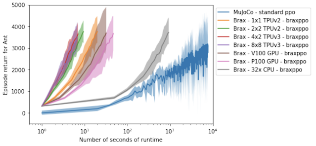
In the graph below, the blue line represents a standard workstation setup, where a learner runs on the GPU and the simulator runs on the CPU. We see that the time it takes to train an ant to run with reasonable proficiency (a score of 4000 on the y axis) drops from about 3 hours for the blue line, to about 10 seconds using Brax on accelerator hardware. It’s interesting to note that even on CPU alone (the grey line), Brax performs more than an order of magnitude faster, benefitting from learner and simulator both sitting in the same process.

Brax’s optimized PPO versus a standard GPU-backed PPO learning the MuJoCo-Ant-v2 environment, evaluated for 10 million steps. Note the x-axis is log-wallclock-time in seconds. Shaded region indicates lowest and highest performing seeds over 5 replicas, and solid line indicates mean.

Physics Fidelity
Designing a simulator that matches the behavior of the real world is a known hard problem that this work does not address. Nevertheless, it is useful to compare Brax to a reference simulator to ensure it is producing output that is at least as valid. In this case, we again compare Brax to MuJoCo, which is well-regarded for its simulation quality. We expect to see that, all else being equal, a policy has a similar reward trajectory whether trained in MuJoCo or Brax.

MuJoCo-Ant-v2 vs. Brax Ant, showing the number of environment steps plotted against the average episode score achieved for the environment. Both environments were trained with the same standard implementation of SAC. Shaded region indicates lowest and highest performing seeds over five runs, and solid line indicates the mean.

These curves show that as the reward rises at about the same rate for both simulators, both engines compute physics with a comparable level of complexity or difficulty to solve. And as both curves top out at about the same reward, we have confidence that the same general physical limits apply to agents operating to the best of their ability in either simulation.

We can also measure Brax’s ability to conserve linear momentum, angular momentum, and energy.

Linear momentum (left), angular momentum (middle), and energy (right) non-conservation scaling for Brax as well as several other physics engines. The y-axis indicates drift from the expected calculation (higher is smaller drift, which is better), and the x axis indicates the amount of time being simulated.

This measure of physics simulation quality was first proposed by the authors of MuJoCo as a way to understand how the simulation drifts off course as it is tasked with computing larger and larger time steps. Here, Brax performs similarly as its neighbors.

Conclusion
We invite researchers to perform a more qualitative measure of Brax’s physics fidelity by training their own policies in the Brax Training Colab. The learned trajectories are recognizably similar to those seen in OpenAI Gym.

Our work makes fast, scalable RL and robotics research much more accessible — what was formerly only possible via large compute clusters can now be run on workstations, or for free via hosted Google Colaboratory. Our Github repository includes not only the Brax simulation engine, but also a host of reference RL algorithms for fast training. We can’t wait to see what kind of new research Brax enables.

Acknowledgements
We'd like to thank our paper co-authors: Anton Raichuk, Sertan Girgin, Igor Mordatch, and Olivier Bachem. We also thank Erwin Coumans for advice on building physics engines, Blake Hechtman and James Bradbury for providing optimization help with JAX and XLA, and Luke Metz and Shane Gu for their advice. We’d also like to thank Vijay Sundaram, Wright Bagwell, Matt Leffler, Gavin Dodd, Brad Mckee, and Logan Olson, for helping to incubate this project.


1 Due to the complexity of the real world, there is also ongoing research exploring the physics of deformable bodies

Source: Google AI Blog


From Vision to Language: Semi-supervised Learning in Action…at Scale

Supervised learning, the machine learning task of training predictive models using data points with known outcomes (i.e., labeled data), is generally the preferred approach in industry because of its simplicity. However, supervised learning requires accurately labeled data, the collection of which is often labor intensive. In addition, as model efficiency improves with better architectures, algorithms, and hardware (GPUs / TPUs), training large models to achieve better quality becomes more accessible, which, in turn, requires even more labeled data for continued progress.

To mitigate such data acquisition challenges, semi-supervised learning, a machine learning paradigm that combines a small amount of labeled data with a large amount of unlabeled data, has recently seen success with methods such as UDA, SimCLR, and many others. In our previous work, we demonstrated for the first time that a semi-supervised learning approach, Noisy Student, can achieve state-of-the-art performance on ImageNet, a large-scale academic benchmark for image classification, by utilizing many more unlabeled examples.

Inspired by these results, today we are excited to present semi-supervised distillation (SSD), a simplified version of Noisy Student, and demonstrate its successful application to the language domain. We apply SSD to language understanding within the context of Google Search, resulting in high performance gains. This is the first successful instance of semi-supervised learning applied at such a large scale and demonstrates the potential impact of such approaches for production-scale systems.

Noisy Student Training
Prior to our development of Noisy Student, there was a large body of research into semi-supervised learning. In spite of this extensive research, however, such systems typically worked well only in the low-data regime, e.g., CIFAR, SVHN, and 10% ImageNet. When labeled data were abundant, such models were unable to compete with fully supervised learning systems, which prevented semi-supervised approaches from being applied to important applications in production, such as search engines and self-driving cars. This shortcoming motivated our development of Noisy Student Training, a semi-supervised learning approach that worked well in the high-data regime, and at the time achieved state-of-the-art accuracy on ImageNet using 130M additional unlabeled images.

Noisy Student Training has 4 simple steps:

  1. Train a classifier (the teacher) on labeled data.
  2. The teacher then infers pseudo-labels on a much larger unlabeled dataset.
  3. Then, it trains a larger classifier on the combined labeled and pseudo-labeled data, while also adding noise (noisy student).
  4. (Optional) Going back to step 2, the student may be used as a new teacher.
An illustration of Noisy Student Training through four simple steps. We use two types of noise: model noise (DropoutStochastic Depth) and input noise (data augmentation, such as RandAugment).

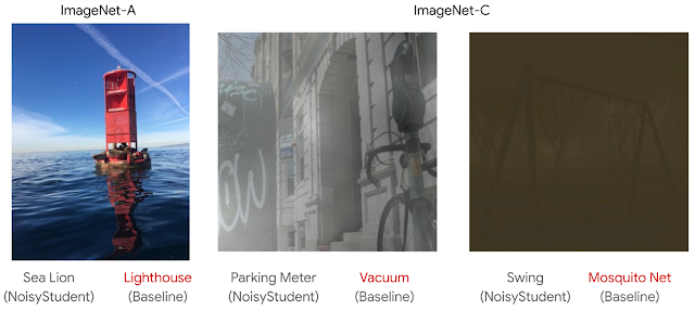
One can view Noisy Student as a form of self-training, because the model generates pseudo-labels with which it retrains itself to improve performance. A surprising property of Noisy Student Training is that the trained models work extremely well on robustness test sets for which it was not optimized, including ImageNet-A, ImageNet-C, and ImageNet-P. We hypothesize that the noise added during training not only helps with the learning, but also makes the model more robust.

Examples of images that are classified incorrectly by the baseline model, but correctly by Noisy Student. Left: An unmodified image from ImageNet-A. Middle and Right: Images with noise added, selected from ImageNet-C. For more examples including ImageNet-P, please see the paper.

Connections to Knowledge Distillation
Noisy Student is similar to knowledge distillation, which is a process of transferring knowledge from a large model (i.e., the teacher) to a smaller model (the student). The goal of distillation is to improve speed in order to build a model that is fast to run in production without sacrificing much in quality compared to the teacher. The simplest setup for distillation involves a single teacher and uses the same data, but in practice, one can use multiple teachers or a separate dataset for the student.

Simple illustrations of Noisy Student and knowledge distillation.

Unlike Noisy Student, knowledge distillation does not add noise during training (e.g., data augmentation or model regularization) and typically involves a smaller student model. In contrast, one can think of Noisy Student as the process of “knowledge expansion”.

Semi-Supervised Distillation
Another strategy for training production models is to apply Noisy Student training twice: first to get a larger teacher model T’ and then to derive a smaller student S. This approach produces a model that is better than either training with supervised learning or with Noisy Student training alone. Specifically, when applied to the vision domain for a family of EfficientNet models, ranging from EfficientNet-B0 with 5.3M parameters to EfficientNet-B7 with 66M parameters, this strategy achieves much better performance for each given model size (see Table 9 of the Noisy Student paper for more details).

Noisy Student training needs data augmentation, e.g., RandAugment (for vision) or SpecAugment (for speech), to work well. But in certain applications, e.g., natural language processing, such types of input noise are not readily available. For those applications, Noisy Student Training can be simplified to have no noise. In that case, the above two-stage process becomes a simpler method, which we call Semi-Supervised Distillation (SSD). First, the teacher model infers pseudo-labels on the unlabeled dataset from which we then train a new teacher model (T’) that is of equal-or-larger size than the original teacher model. This step, which is essentially self-training, is then followed by knowledge distillation to produce a smaller student model for production.

An illustration of Semi-Supervised Distillation (SSD), a 2-stage process that self-trains an equal-or-larger teacher (T’) before distilling to a student (S).

Improving Search
Having succeeded in the vision domain, an application in the language understanding domain, like Google Search, is a logical next step with broader user impact. In this case, we focus on an important ranking component in Search, which builds on BERT to better understand languages. This task turns out to be well-suited for SSD. Indeed, applying SSD to the ranking component to better understand the relevance of candidate search results to queries achieved one of the highest performance gains among top launches at Search in 2020. Below is an example of a query where the improved model demonstrates better language understanding.

With the implementation of SSD, Search is able to find documents that are more relevant to user queries.

Future Research & Challenges
We have presented a successful instance of semi-supervised distillation (SSD) in the production scale setting of Search. We believe SSD will continue changing the landscape of machine learning usage in the industry from predominantly supervised learning to semi-supervised learning. While our results are promising, there is still much research needed in how to efficiently utilize unlabeled examples in the real world, which is often noisy, and apply them to various domains.

Acknowledgements
Zhenshuai Ding, Yanping Huang, Elizabeth Tucker, Hai Qian, and Steve He contributed immensely to this successful launch. The project would not have succeeded without contributions from members of both the Brain and Search teams: Shuyuan Zhang, Rohan Anil, Zhifeng Chen, Rigel Swavely, Chris Waterson, Avinash Atreya. Thanks to Qizhe Xie and Zihang Dai for feedback on the work. Also, thanks to Quoc Le, Yonghui Wu, Sundeep Tirumalareddy, Alexander Grushetsky, Pandu Nayak for their leadership support.

Source: Google AI Blog


Reducing the Computational Cost of Deep Reinforcement Learning Research

It is widely accepted that the enormous growth of deep reinforcement learning research, which combines traditional reinforcement learning with deep neural networks, began with the publication of the seminal DQN algorithm. This paper demonstrated the potential of this combination, showing that it could produce agents that could play a number of Atari 2600 games very effectively. Since then, there have been several approaches that have built on and improved the original DQN. The popular Rainbow algorithm combined a number of these recent advances to achieve state-of-the-art performance on the ALE benchmark. This advance, however, came at a very high computational cost, which has the unfortunate side effect of widening the gap between those with ample access to computational resources and those without.

In “Revisiting Rainbow: Promoting more Insightful and Inclusive Deep Reinforcement Learning Research”, to be presented at ICML 2021, we revisit this algorithm on a set of small- and medium-sized tasks. We first discuss the computational cost associated with the Rainbow algorithm. We explore how the same conclusions regarding the benefits of combining the various algorithmic components can be reached with smaller-scale experiments, and further generalize that idea to how research done on a smaller computational budget can provide valuable scientific insights.

The Cost of Rainbow
A major reason for the computational cost of Rainbow is that the standards in academic publishing often require evaluating new algorithms on large benchmarks like ALE, which consists of 57 Atari 2600 games that reinforcement learning agents may learn to play. For a typical game, it takes roughly five days to train a model using a Tesla P100 GPU. Furthermore, if one wants to establish meaningful confidence bounds, it is common to perform at least five independent runs. Thus, to train Rainbow on the full suite of 57 games required around 34,200 GPU hours (or 1425 days) in order to provide convincing empirical performance statistics. In other words, such experiments are only feasible if one is able to train on multiple GPUs in parallel, which can be prohibitive for smaller research groups.

Revisiting Rainbow
As in the original Rainbow paper, we evaluate the effect of adding the following components to the original DQN algorithm: double Q-learning, prioritized experience replay, dueling networks, multi-step learning, distributional RL, and noisy nets.

We evaluate on a set of four classic control environments, which can be fully trained in 10-20 minutes (compared to five days for ALE games):

Upper left: In CartPole, the task is to balance a pole on a cart that the agent can move left and right. Upper right: In Acrobot, there are two arms and two joints, where the agent applies force to the joint between the two arms in order to raise the lower arm above a threshold. Lower left: In LunarLander, the agent is meant to land the spaceship between the two flags. Lower right: In MountainCar, the agent must build up momentum between two hills to drive to the top of the rightmost hill.

We investigated the effect of both independently adding each of the components to DQN, as well as removing each from the full Rainbow algorithm. As in the original Rainbow paper, we find that, in aggregate, the addition of each of these algorithms does improve learning over the base DQN. However, we also found some important differences, such as the fact that distributional RL — commonly thought to be a positive addition on its own — does not always yield improvements on its own. Indeed, in contrast to the ALE results in the Rainbow paper, in the classic control environments, distributional RL only yields an improvement when combined with another component.

Each plot shows the training progress when adding the various components to DQN. The x-axis is training steps,the y-axis is performance (higher is better).
Each plot shows the training progress when removing the various components from Rainbow. The x-axis is training steps,the y-axis is performance (higher is better).

We also re-ran the Rainbow experiments on the MinAtar environment, which consists of a set of five miniaturized Atari games, and found qualitatively similar results. The MinAtar games are roughly 10 times faster to train than the regular Atari 2600 games on which the original Rainbow algorithm was evaluated, but still share some interesting aspects, such as game dynamics and having pixel-based inputs to the agent. As such, they provide a challenging mid-level environment, in between the classic control and the full Atari 2600 games.

When viewed in aggregate, we find our results to be consistent with those of the original Rainbow paper — the impact resulting from each algorithmic component can vary from environment to environment. If we were to suggest a single agent that balances the tradeoffs of the different algorithmic components, our version of Rainbow would likely be consistent with the original, in that combining all components produces a better overall agent. However, there are important details in the variations of the different algorithmic components that merit a more thorough investigation.

Beyond the Rainbow
When DQN was introduced, it made use of the Huber loss and the RMSProp Optimizer. It has been common practice for researchers to use these same choices when building on DQN, as most of their effort is spent on other algorithmic design decisions. In the spirit of reassessing these assumptions, we revisited the loss function and optimizer used by DQN on a lower-cost, small-scale classic control and MinAtar environments. We ran some initial experiments using the Adam optimizer, which has lately been the most popular optimizer choice, combined with a simpler loss function, the mean-squared error loss (MSE). Since the selection of optimizer and loss function is often overlooked when developing a new algorithm, we were surprised to see that we observed a dramatic improvement on all the classic control and MinAtar environments.

We thus decided to evaluate the different ways of combining the two optimizers (RMSProp and Adam) with the two losses (Huber and MSE) on the full ALE suite (60 Atari 2600 games). We found that Adam+MSE is a superior combination than RMSProp+Huber.

Measuring the improvement Adam+MSE gives over the default DQN settings (RMSProp + Huber); higher is better.

Additionally, when comparing the various optimizer-loss combinations, we find that when using RMSProp, the Huber loss tends to perform better than MSE (illustrated by the gap between the solid and dotted orange lines).

Normalized scores aggregated over all 60 Atari 2600 games, comparing the different optimizer-loss combinations.

Conclusion
On a limited computational budget we were able to reproduce, at a high-level, the findings of the Rainbow paper and uncover new and interesting phenomena. Evidently it is much easier to revisit something than to discover it in the first place. Our intent with this work, however, was to argue for the relevance and significance of empirical research on small- and medium-scale environments. We believe that these less computationally intensive environments lend themselves well to a more critical and thorough analysis of the performance, behaviors, and intricacies of new algorithms.

We are by no means calling for less emphasis to be placed on large-scale benchmarks. We are simply urging researchers to consider smaller-scale environments as a valuable tool in their investigations, and reviewers to avoid dismissing empirical work that focuses on smaller-scale environments. By doing so, in addition to reducing the environmental impact of our experiments, we will get both a clearer picture of the research landscape and reduce the barriers for researchers from diverse and often underresourced communities, which can only help make our community and scientific advances stronger.

Acknowledgments
Thank you to Johan, the first author of this paper, for his hard work and persistence in seeing this through! We would also like to thank Marlos C. Machado, Sara Hooker, Matthieu Geist, Nino Vieillard, Hado van Hasselt, Eleni Triantafillou, and Brian Tanner for their insightful comments on this work.

Source: Google AI Blog


Quickly Training Game-Playing Agents with Machine Learning

In the last two decades, dramatic advances in compute and connectivity have allowed game developers to create works of ever-increasing scope and complexity. Simple linear levels have evolved into photorealistic open worlds, procedural algorithms have enabled games with unprecedented variety, and expanding internet access has transformed games into dynamic online services. Unfortunately, scope and complexity have grown more rapidly than the size of quality assurance teams or the capabilities of traditional automated testing. This poses a challenge to both product quality (such as delayed releases and post-launch patches) and developer quality of life.

Machine learning (ML) techniques offer a possible solution, as they have demonstrated the potential to profoundly impact game development flows – they can help designers balance their game and empower artists to produce high-quality assets in a fraction of the time traditionally required. Furthermore, they can be used to train challenging opponents that can compete at the highest levels of play. Yet some ML techniques can pose requirements that currently make them impractical for production game teams, including the design of game-specific network architectures, the development of expertise in implementing ML algorithms, or the generation of billions of frames of training data. Conversely, game developers operate in a setting that offers unique advantages to leverage ML techniques, such as direct access to the game source, an abundance of expert demonstrations, and the uniquely interactive nature of video games.

Today, we present a ML-based system that game developers can use to quickly and efficiently train game-testing agents, helping developers find serious bugs quickly while allowing human testers to focus on more complex and intricate problems. The resulting solution requires no ML expertise, works on many of the most popular game genres, and can train an ML policy, which generates game actions from game state, in less than an hour on a single game instance. We have also released an open source library that demonstrates a functional application of these techniques.

Supported genres include arcade, action/adventure, and racing games.

The Right Tool for the Right Job
The most elemental form of video game testing is to simply play the game. A lot. Many of the most serious bugs (such as crashes or falling out of the world) are easy to detect and fix; the challenge is finding them within the vast state space of a modern game. As such, we decided to focus on training a system that could “just play the game” at scale.

We found that the most effective way to do this was not to try to train a single, super effective agent that could play the entire game from end-to-end, but to provide developers with the ability to train an ensemble of game-testing agents, each of which could effectively accomplish tasks of a few minutes each, which game developers refer to as “gameplay loops”.

These core gameplay behaviors are often expensive to program through traditional means, but are much more efficient to train than a single end-to-end ML model. In practice, commercial games create longer loops by repeating and remixing core gameplay loops, which means that developers can test large stretches of gameplay by combining ML policies with a small amount of simple scripting.

Simulation-centric, Semantic API
One of the most fundamental challenges in applying ML to game development is bridging the chasm between the simulation-centric world of video games and the data-centric world of ML. Rather than ask developers to directly convert the game state into custom, low-level ML features (which would be too labor intensive) or attempting to learn from raw pixels (which would require too much data to train), our system provides developers with an idiomatic, game-developer friendly API that allows them to describe their game in terms of the essential state that a player observes and the semantic actions they can perform. All of this information is expressed via concepts that are familiar to game developers, such as entities, raycasts, 3D positions and rotations, buttons and joysticks.

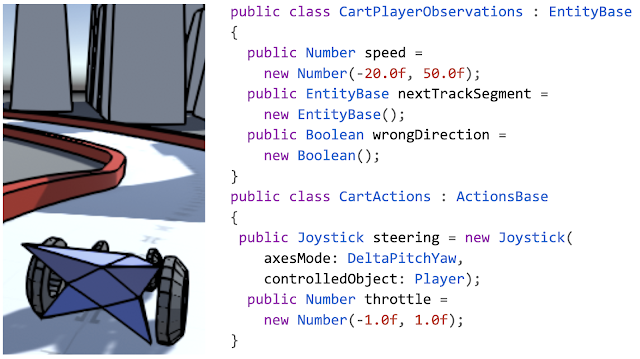
As you can see in the example below, the API allows the specification of observations and actions in just a few lines of code.

Example actions and observations for a racing game.

From API to Neural Network
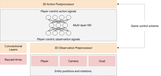
This high level, semantic API is not just easy to use but also allows the system to flexibly adapt to the specific game being developed – the specific combination of API building blocks employed by the game developer informs our choice of network architecture, since it provides information about the type of gaming scenario in which the system is deployed. Some examples of this include: handling action outputs differently depending on whether they represent a digital button or analog joystick, or using techniques from image processing to handle observations that result from an agent probing its environment with raycasts (similar to how autonomous vehicles probe their environment with LIDAR).

Our API is sufficiently general to allow modeling of many common control-schemes (the configuration of action outputs that control movement) in games, such as first-person games, third-person games with camera-relative controls, racing games, twin stick shooters, etc. Since 3D movement and aiming are often an integral aspect of gameplay in general, we create networks that automatically tend towards simple behaviors such as aiming, approach or avoidance in these games. The system accomplishes this by analyzing the game’s control scheme to create neural network layers that perform custom processing of observations and actions in that game. For example, positions and rotations of objects in the world are automatically translated into directions and distances from the point of view of the AI-controlled game entity. This transformation typically increases the speed of learning and helps the learned network generalize better.

An example neural network generated for a game with joystick controls and raycast inputs. Depending on the inputs (red) and the control scheme, the system generates custom pre- and post-processing layers (orange).

Learning From The Experts in Real Time
After generating a neural network architecture, the network needs to be trained to play the game using an appropriate choice of learning algorithm.

Reinforcement learning (RL), in which an ML policy is trained directly to maximize a reward, may seem like the obvious choice since they have been successfully used to train highly competent ML policies for games. However, RL algorithms tend to require more data than a single game instance can produce in a reasonable amount of time, and achieving good results in a new domain often requires hyperparameter tuning and strong ML domain knowledge.

Instead, we found that imitation learning (IL), which trains ML policies based by observing experts play the game, works well for our use case. Unlike RL, where the agent needs to discover a good policy on its own, IL only needs to recreate the behavior of a human expert. Since game developers and testers are experts in their own games, they can easily provide demonstrations of how to play the game.

We use an IL approach inspired by the DAgger algorithm, which allows us to take advantage of video games’ most compelling quality – interactivity. Thanks to the reductions in training time and data requirements enabled by our semantic API, training is effectively realtime, giving a developer the ability to fluidly switch between providing gameplay demonstrations and watching the system play. This results in a natural feedback loop, in which a developer iteratively provides corrections to a continuous stream of ML policies.

From the developer’s perspective, providing a demonstration or a correction to faulty behavior is as simple as picking up the controller and starting to play the game. Once they are done, they can put the controller down and watch the ML policy play. The result is a training experience that is real-time, interactive, highly experiential, and, very often, more than a little fun.

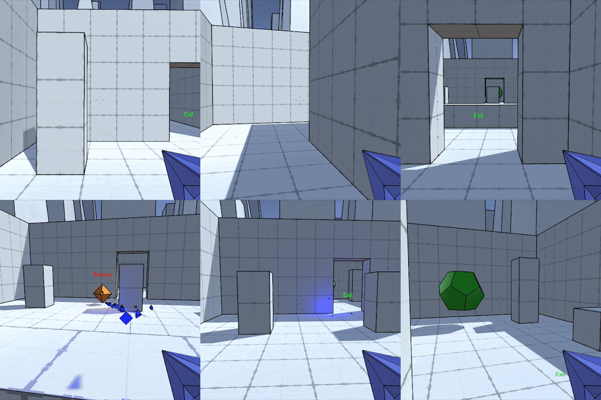
ML policy for an FPS game, trained with our system.

Conclusion
We present a system which combines a high-level semantic API with a DAgger-inspired interactive training flow that enables training of useful ML policies for video game testing in a wide variety of genres. We have released an open source library as a functional illustration of our system. No ML expertise is required and training of agents for test applications often takes less than an hour on a single developer machine. We hope that this work will help inspire the development of ML techniques that can be deployed in real-world game-development flows in ways that are accessible, effective, and fun to use.

Acknowledgements
We’d like to thank the core members of the project: Dexter Allen, Leopold Haller, Nathan Martz, Hernan Moraldo, Stewart Miles and Hina Sakazaki. Training algorithms are provided by TF Agents, and on-device inference by TF Lite. Special thanks to our research advisors, Olivier Bachem, Erik Frey, and Toby Pohlen, and to Eugene Brevdo, Jared Duke, Oscar Ramirez and Neal Wu who provided helpful guidance and support.

Source: Google AI Blog


Take All Your Pictures to the Cleaners, with Google Photos Noise and Blur Reduction

Despite recent leaps in imaging technology, especially on mobile devices, image noise and limited sharpness remain two of the most important levers for improving the visual quality of a photograph. These are particularly relevant when taking pictures in poor light conditions, where cameras may compensate by increasing the ISO or slowing the shutter speed, thereby exacerbating the presence of noise and, at times, increasing image blur. Noise can be associated with the particle nature of light (shot noise) or be introduced by electronic components during the readout process (read noise). The captured noisy signal is then processed by the camera image processor (ISP) and later may be further enhanced, amplified, or distorted by a photographic editing process. Image blur can be caused by a wide variety of phenomena, from inadvertent camera shake during capture, an incorrect setting of the camera’s focus (automatic or not), or due to the finite lens aperture, sensor resolution or the camera’s image processing.

It is far easier to minimize the effects of noise and blur within a camera pipeline, where details of the sensor, optical hardware and software blocks are understood. However, when presented with an image produced from an arbitrary (possibly unknown) camera, improving noise and sharpness becomes much more challenging due to the lack of detailed knowledge and access to the internal parameters of the camera. In most situations, these two problems are intrinsically related: noise reduction tends to eliminate fine structures along with unwanted details, while blur reduction seeks to boost structures and fine details. This interconnectedness increases the difficulty of developing image enhancement techniques that are computationally efficient to run on mobile devices.

Today, we present a new approach for camera-agnostic estimation and elimination of noise and blur that can improve the quality of most images. We developed a pull-push denoising algorithm that is paired with a deblurring method, called polyblur. Both of these components are designed to maximize computational efficiency, so users can successfully enhance the quality of a multi-megapixel image in milliseconds on a mobile device. These noise and blur reduction strategies are critical components of the recent Google Photos editor updates, which includes “Denoise” and “Sharpen” tools that enable users to enhance images that may have been captured under less than ideal conditions, or with older devices that may have had more noisy sensors or less sharp optics.

A demonstration of the “Denoise” and “Sharpen” tools now available in the Google Photos editor.

How Noisy is An Image?
In order to accurately process a photographic image and successfully reduce the unwanted effects of noise and blur, it is vitally important to first characterize the types and levels of noise and blur found in the image. So, a camera-agnostic approach for noise reduction begins by formulating a method to gauge the strength of noise at the pixel level from any given image, regardless of the device that created it. The noise level is modeled as a function of the brightness of the underlying pixel. That is, for each possible brightness level, the model estimates a corresponding noise level in a manner agnostic to either the actual source of the noise or the processing pipeline.

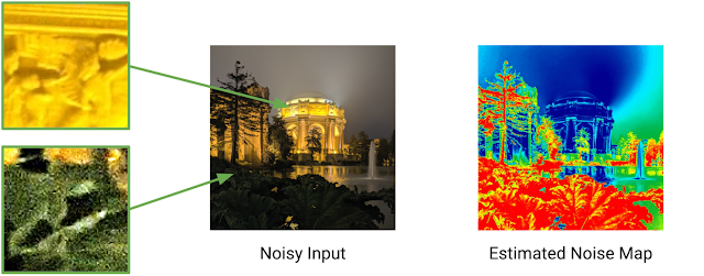
To estimate this brightness-based noise level, we sample a number of small patches across the image and measure the noise level within each patch, after roughly removing any underlying structure in the image. This process is repeated at multiple scales, making it robust to artifacts that may arise from compression, image resizing, or other non-linear camera processing operations.

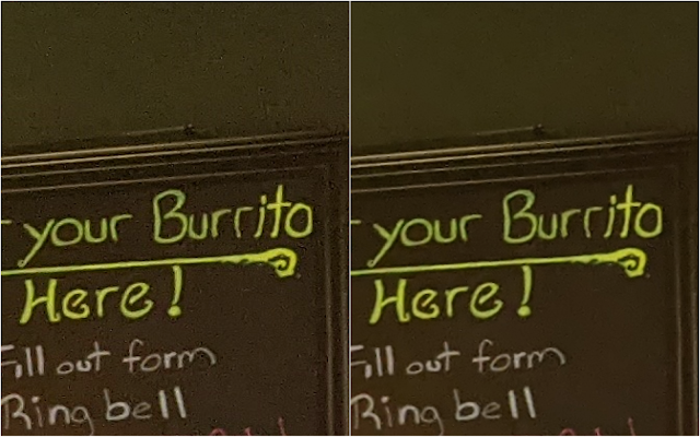
The two segments on the left illustrate signal-dependent noise present in the input image (center). The noise is more prominent in the bottom, darker crop and is unrelated to the underlying structure, but rather to the light level. Such image segments are sampled and processed to generate the spatially-varying noise map (right) where red indicates more noise is present.

Reducing Noise Selectively with a Pull-Push Method
We take advantage of self-similarity of patches across the image to denoise with high fidelity. The general principle behind such so-called “non-local” denoising is that noisy pixels can be denoised by averaging pixels with similar local structure. However, these approaches typically incur high computational costs because they require a brute force search for pixels with similar local structure, making them impractical for on-device use. In our “pull-push” approach1, the algorithmic complexity is decoupled from the size of filter footprints thanks to effective information propagation across spatial scales.

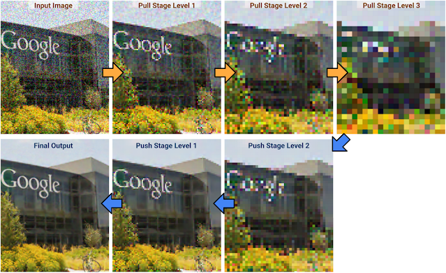
The first step in pull-push is to build an image pyramid (i.e., multiscale representation) in which each successive level is generated recursively by a “pull” filter (analogous to downsampling). This filter uses a per-pixel weighting scheme to selectively combine existing noisy pixels together based on their patch similarities and estimated noise, thus reducing the noise at each successive, “coarser” level. Pixels at coarser levels (i.e., with lower resolution) pull and aggregate only compatible pixels from higher resolution, “finer” levels. In addition to this, each merged pixel in the coarser layers also includes an estimated reliability measure computed from the similarity weights used to generate it. Thus, merged pixels provide a simple per-pixel, per-level characterization of the image and its local statistics. By efficiently propagating this information through each level (i.e., each spatial scale), we are able to track a model of the neighborhood statistics for increasingly larger regions in a multiscale manner.

After the pull stage is evaluated to the coarsest level, the “push” stage fuses the results, starting from the coarsest level and generating finer levels iteratively. At a given scale, the push stage generates “filtered” pixels following a process similar to that of the pull stage, but going from coarse to finer levels. The pixels at each level are fused with those of coarser levels by doing a weighted average of same-level pixels along with coarser-level filtered pixels using the respective reliability weights. This enables us to reduce pixel noise while preserving local structure, because only average reliable information is included. This selective filtering and reliability (i.e. information) multiscale propagation is what makes push-pull different from existing frameworks.

This series of images shows how filtering progresses through the pull-push process. Coarser level pixels pull and aggregate only compatible pixels from finer levels, as opposed to the traditional multiscale approaches using a fixed (non-data dependent) kernel. Notice how the noise is reduced throughout the stages.

The pull-push approach has a low computational cost, because the algorithm to selectively filter similar pixels over a very large neighborhood has a complexity that is only linear with the number of image pixels. In practice, the quality of this denoising approach is comparable to traditional non-local methods with much larger kernel footprints, but operates at a fraction of the computational cost.

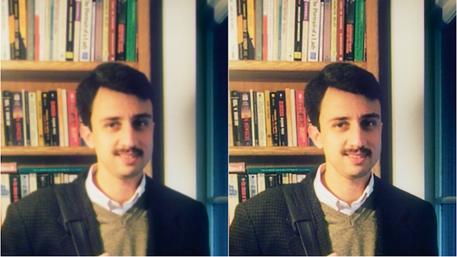
Image enhanced using the pull-push denoising method.

How Blurry Is an Image?
An image with poor sharpness can be thought of as being a more pristine latent image that was operated on by a blur kernel. So, if one can identify the blur kernel, it can be used to reduce the effect. This is referred to as “deblurring”, i.e., the removal or reduction of an undesired blur effect induced by a particular kernel on a particular image. In contrast, “sharpening” refers to applying a sharpening filter, built from scratch and without reference to any particular image or blur kernel. Typical sharpening filters are also, in general, local operations that do not take account of any other information from other parts of the image, whereas deblurring algorithms estimate the blur from the whole image. Unlike arbitrary sharpening, which can result in worse image quality when applied to an image that is already sharp, deblurring a sharp image with a blur kernel accurately estimated from the image itself will have very little effect.

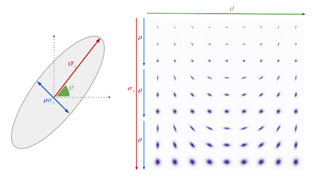
We specifically target relatively mild blur, as this scenario is more technically tractable, more computationally efficient, and produces consistent results. We model the blur kernel as an anisotropic (elliptical) Gaussian kernel, specified by three parameters that control the strength, direction and aspect ratio of the blur.

Gaussian blur model and example blur kernels. Each row of the plot on the right represents possible combinations of σ0, ρ and θ. We show three different σ0 values with three different ρ values for each.

Computing and removing blur without noticeable delay for the user requires an algorithm that is much more computationally efficient than existing approaches, which typically cannot be executed on a mobile device. We rely on an intriguing empirical observation: the maximal value of the image gradient across all directions at any point in a sharp image follows a particular distribution. Finding the maximum gradient value is efficient, and can yield a reliable estimate of the strength of the blur in the given direction. With this information in hand, we can directly recover the parameters that characterize the blur.

Polyblur: Removing Blur by Re-blurring
To recover the sharp image given the estimated blur, we would (in theory) need to solve a numerically unstable inverse problem (i.e., deblurring). The inversion problem grows exponentially more unstable with the strength of the blur. As such, we target the case of mild blur removal. That is, we assume that the image at hand is not so blurry as to be beyond practical repair. This enables a more practical approach — by carefully combining different re-applications of an operator we can approximate its inverse.

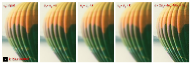
Mild blur, as shown in these examples, can be effectively removed by combining multiple applications of the estimated blur.

This means, rather counterintuitively, that we can deblur an image by re-blurring it several times with the estimated blur kernel. Each application of the (estimated) blur corresponds to a first order polynomial, and the repeated applications (adding or subtracting) correspond to higher order terms in a polynomial. A key aspect of this approach, which we call polyblur, is that it is very fast, because it only requires a few applications of the blur itself. This allows it to operate on megapixel images in a fraction of a second on a typical mobile device. The degree of the polynomial and its coefficients are set to invert the blur without boosting noise and other unwanted artifacts.

The deblurred image is generated by adding and subtracting multiple re-applications of the estimated blur (polyblur).

Integration with Google Photos
The innovations described here have been integrated and made available to users in the Google Photos image editor in two new adjustment sliders called “Denoise” and “Sharpen”. These features allow users to improve the quality of everyday images, from any capture device. The features often complement each other, allowing both denoising to reduce unwanted artifacts, and sharpening to bring clarity to the image subjects. Try using this pair of tools in tandem in your images for best results. To learn more about the details of the work described here, check out our papers on polyblur and pull-push denoising. To see some examples of the effect of our denoising and sharpening up close, have a look at the images in this album.

Acknowledgements
The authors gratefully acknowledge the contributions of Ignacio Garcia-Dorado, Ryan Campbell, Damien Kelly, Peyman Milanfar, and John Isidoro. We are also thankful for support and feedback from Navin Sarma, Zachary Senzer, Brandon Ruffin, and Michael Milne.


1 The original pull-push algorithm was developed as an efficient scattered data interpolation method to estimate and fill in the missing pixels in an image where only a subset of the pixels are specified. Here, we extend its methodology and present a data-dependent multiscale algorithm for denoising images efficiently. 

Source: Google AI Blog


Achieving Precision in Quantum Material Simulations

In fall of 2019, we demonstrated that the Sycamore quantum processor could outperform the most powerful classical computers when applied to a tailor-made problem. The next challenge is to extend this result to solve practical problems in materials science, chemistry and physics. But going beyond the capabilities of classical computers for these problems is challenging and will require new insights to achieve state-of-the-art accuracy. Generally, the difficulty in performing quantum simulations of such physical problems is rooted in the wave nature of quantum particles, where deviations in the initial setup, interference from the environment, or small errors in the calculations can lead to large deviations in the computational result.

In two upcoming publications, we outline a blueprint for achieving record levels of precision for the task of simulating quantum materials. In the first work, we consider one-dimensional systems, like thin wires, and demonstrate how to accurately compute electronic properties, such as current and conductance. In the second work, we show how to map the Fermi-Hubbard model, which describes interacting electrons, to a quantum processor in order to simulate important physical properties. These works take a significant step towards realizing our long-term goal of simulating more complex systems with practical applications, like batteries and pharmaceuticals.

A bottom view of one of the quantum dilution refrigerators during maintenance. During the operation, the microwave wires that are floating in this image are connected to the quantum processor, e.g., the Sycamore chip, bringing the temperature of the lowest stage to a few tens of milli-degrees above absolute zero temperature.

Computing Electronic Properties of Quantum Materials
In “Accurately computing electronic properties of a quantum ring”, to be published in Nature, we show how to reconstruct key electronic properties of quantum materials. The focus of this work is on one-dimensional conductors, which we simulate by forming a loop out of 18 qubits on the Sycamore processor in order to mimic a very narrow wire. We illustrate the underlying physics through a series of simple text-book experiments, starting with a computation of the “band-structure” of this wire, which describes the relationship between the energy and momentum of electrons in the metal. Understanding such structure is a key step in computing electronic properties such as current and conductance. Despite being an 18-qubit algorithm consisting of over 1,400 logical operations, a significant computational task for near-term devices, we are able to achieve a total error as low as 1%.

The key insight enabling this level of accuracy stems from robust properties of the Fourier transform. The quantum signal that we measure oscillates in time with a small number of frequencies. Taking a Fourier transform of this signal reveals peaks at the oscillation frequencies (in this case, the energy of electrons in the wire). While experimental imperfections affect the height of the observed peaks (corresponding to the strength of the oscillation), the center frequencies are robust to these errors. On the other hand, the center frequencies are especially sensitive to the physical properties of the wire that we hope to study (e.g., revealing small disorders in the local electric field felt by the electrons). The essence of our work is that studying quantum signals in the Fourier domain enables robust protection against experimental errors while providing a sensitive probe of the underlying quantum system.

(Left) Schematic of the 54-qubit quantum processor, Sycamore. Qubits are shown as gray crosses and tunable couplers as blue squares. Eighteen of the qubits are isolated to form a ring. (Middle) Fourier transform of the measured quantum signal. Peaks in the Fourier spectrum correspond to the energy of electrons in the ring. Each peak can be associated with a traveling wave that has fixed momentum. (Right) The center frequency of each peak (corresponding to the energy of electrons in the wire) is plotted versus the peak index (corresponding to the momentum). The measured relationship between energy and momentum is referred to as the ‘band structure’ of the quantum wire and provides valuable information about electronic properties of the material, such as current and conductance.

Quantum Simulation of the Fermi-Hubbard Model
In “Observation of separated dynamics of charge and spin in the Fermi-Hubbard model”, we focus on the dynamics of interacting electrons. Interactions between particles give rise to novel phenomena such as high temperature superconductivity and spin-charge separation. The simplest model that captures this behavior is known as the Fermi-Hubbard model. In materials such as metals, the atomic nuclei form a crystalline lattice and electrons hop from lattice site to lattice site carrying electrical current. In order to accurately model these systems, it is necessary to include the repulsion that electrons feel when getting close to one another. The Fermi-Hubbard model captures this physics with two simple parameters that describe the hopping rate (J) and the repulsion strength (U).

We realize the dynamics of this model by mapping the two physical parameters to logical operations on the qubits of the processor. Using these operations, we simulate a state of the electrons where both the electron charge and spin densities are peaked near the center of the qubit array. As the system evolves, the charge and spin densities spread at different rates due to the strong correlations between electrons. Our results provide an intuitive picture of interacting electrons and serve as a benchmark for simulating quantum materials with superconducting qubits.

(Left top) Illustration of the one-dimensional Fermi-Hubbard model in a periodic potential. Electrons are shown in blue, with their spin indicated by the connected arrow. J, the distance between troughs in the electric potential field, reflects the “hopping” rate, i.e., the rate at which electrons transition from one trough in the potential to another, and U, the amplitude, represents the strength of repulsion between electrons. (Left bottom) The simulation of the model on a qubit ladder, where each qubit (square) represents a fermionic state with spin-up or spin-down (arrows). (Right) Time evolution of the model reveals separated spreading rates of charge and spin. Points and solid lines represent experimental and numerical exact results, respectively. At t = 0, the charge and spin densities are peaked at the middle sites. At later times, the charge density spreads and reaches the boundaries faster than the spin density.

Conclusion
Quantum processors hold the promise to solve computationally hard tasks beyond the capability of classical approaches. However, in order for these engineered platforms to be considered as serious contenders, they must offer computational accuracy beyond the current state-of-the-art classical methods. In our first experiment, we demonstrate an unprecedented level of accuracy in simulating simple materials, and in our second experiment, we show how to embed realistic models of interacting electrons into a quantum processor. It is our hope that these experimental results help progress the goal of moving beyond the classical computing horizon.

Source: Google AI Blog


A Dataset for Studying Gender Bias in Translation

Advances on neural machine translation (NMT) have enabled more natural and fluid translations, but they still can reflect the societal biases and stereotypes of the data on which they're trained. As such, it is an ongoing goal at Google to develop innovative techniques to reduce gender bias in machine translation, in alignment with our AI Principles.

One research area has been using context from surrounding sentences or passages to improve gender accuracy. This is a challenge because traditional NMT methods translate sentences individually, but gendered information is not always explicitly stated in each individual sentence. For example, in the following passage in Spanish (a language where subjects aren’t always explicitly mentioned), the first sentence refers explicitly to Marie Curie as the subject, but the second one doesn't explicitly mention the subject. In isolation, this second sentence could refer to a person of any gender. When translating to English, however, a pronoun needs to be picked, and the information needed for an accurate translation is in the first sentence.

Spanish Text Translation to English
Marie Curie nació en Varsovia. Fue la primera persona en recibir dos premios Nobel en distintas especialidades. Marie Curie was born in Warsaw. She was the first person to receive two Nobel Prizes in different specialties.

Advancing translation techniques beyond single sentences requires new metrics for measuring progress and new datasets with the most common context-related errors. Adding to this challenge is the fact that translation errors related to gender (such as picking the correct pronoun or having gender agreement) are particularly sensitive, because they may directly refer to people and how they self identify.

To help facilitate progress against the common challenges on contextual translation (e.g., pronoun drop, gender agreement and accurate possessives), we are releasing the Translated Wikipedia Biographies dataset, which can be used to evaluate the gender bias of translation models. Our intent with this release is to support long-term improvements on ML systems focused on pronouns and gender in translation by providing a benchmark in which translations’ accuracy can be measured pre- and post-model changes.

A Source of Common Translation Errors
Because they are well-written, geographically diverse, contain multiple sentences, and refer to subjects in the third person (and so contain plenty of pronouns), Wikipedia biographies offer a high potential for common translation errors associated with gender. These often occur when articles refer to a person explicitly in early sentences of a paragraph, but there is no explicit mention of the person in later sentences. Some examples:

Translation Error     Text     Translation
Pro-drop in Spanish → English    Marie Curie nació en Varsovia. Recibió el Premio Nobel en 1903 y en 1911.     Marie Curie was born in Warsaw. He received the Nobel Prize in 1903 and in 1911.

Neutral possessives in Spanish → English    Marie Curie nació en Varsovia. Su carrera profesional fue desarrollada en Francia.     Marie Curie was born in Warsaw. His professional career was developed in France.

Gender agreement in English → German    Marie Curie was born in Warsaw. The distinguished scientist received the Nobel Prize in 1903 and in 1911.     Marie Curie wurde in Varsovia geboren. Der angesehene Wissenschaftler erhielt 1903 und 1911 den Nobelpreis.

Gender agreement in English → Spanish     Marie Curie was born in Warsaw. The distinguished scientist received the Nobel Prize in 1903 and in 1911.     Marie Curie nació en Varsovia. El distinguido científico recibió el Premio Nobel en 1903 y en 1911.

Building the Dataset
The Translated Wikipedia Biographies dataset has been designed to analyze common gender errors in machine translation, such as those illustrated above. Each instance of the dataset represents a person (identified in the biographies as feminine or masculine), a rock band or a sports team (considered genderless). Each instance is represented by a long text translation of 8 to 15 connected sentences referring to that central subject (the person, rock band, or sports team). Articles are written in native English and have been professionally translated to Spanish and German. For Spanish, translations were optimized for pronoun-drop, so the same set could be used to analyze pro-drop (Spanish → English) and gender agreement (English → Spanish).

The dataset was built by selecting a group of instances that has equal representation across geographies and genders. To do this, we extracted biographies from Wikipedia according to occupation, profession, job and/or activity. To ensure an unbiased selection of occupations, we chose nine occupations that represented a range of stereotypical gender associations (either feminine, masculine, or neither) based on Wikipedia statistics. Then, to mitigate any geography-based bias, we divided all these instances based on geographical diversity. For each occupation category, we looked to have one candidate per region (using regions from census.gov as a proxy of geographical diversity). When an instance was associated with a region, we checked that the selected person had a relevant relationship with a country that belongs to a designated region (nationality, place of birth, lived for a big portion of their life, etc.). By using this criteria, the dataset contains entries about individuals from more than 90 countries and all regions of the world.

Although gender is non-binary, we focused on having equal representation of “feminine” and “masculine” entities. It's worth mentioning that because the entities are represented as such on Wikipedia, the set doesn't include individuals that identify as non-binary, as, unfortunately, there are not enough instances currently represented in Wikipedia to accurately reflect the non-binary community. To label each instance as "feminine" or "masculine" we relied on the biographical information from Wikipedia, which contained gender-specific references to the person (she, he, woman, son, father, etc.).

After applying all these filters, we randomly selected an instance for each occupation-region-gender triplet. For each occupation, there are two biographies (one masculine and one feminine), for each of the seven geographic regions.

Finally, we added 12 instances with no gender. We picked rock bands and sports teams because they are usually referred to by non-gendered third person pronouns (such as “it” or singular “they”). The purpose of including these instances is to study over triggering, i.e., when models learn that they are rewarded for producing gender-specific pronouns, leading them to produce these pronouns in cases where they shouldn't.

Results and Applications
This dataset enables a new method of evaluation for gender bias reduction in machine translations (introduced in a previous post). Because each instance refers to a subject with a known gender, we can compute the accuracy of the gender-specific translations that refer to this subject. This computation is easier when translating into English (cases of languages with pro-drop or neutral pronouns) since computation is mainly based on gender-specific pronouns in English. In these cases, the gender datasets have resulted in a 67% reduction in errors on context-aware models vs. previous models. As mentioned before, the neutral entities have allowed us to discover cases of over triggering like the usage of feminine or masculine pronouns to refer to genderless entities. This new dataset also enables new research directions into the performance of different models across types of occupations or geographic regions.

As an example, the dataset allowed us to discover the following improvements in an excerpt of the translated biography of Marie Curie from Spanish.

Translation result with the previous NMT model.
Translation result with the new contextual model.

Conclusion
This Translated Wikipedia Biographies dataset is the result of our own studies and work on identifying biases associated with gender and machine translation. This set focuses on a specific problem related to gender bias and doesn't aim to cover the whole problem. It's worth mentioning that by releasing this dataset, we don't aim to be prescriptive in determining what's the optimal approach to address gender bias. This contribution aims to foster progress on this challenge across the global research community.

Acknowledgements
The datasets were built with help from Anja Austermann, Melvin Johnson, Michelle Linch, Mengmeng Niu, Mahima Pushkarna, Apu Shah, Romina Stella, and Kellie Webster.

Source: Google AI Blog