Author Archives: Google AI

Pathways Language Model (PaLM): Scaling to 540 Billion Parameters for Breakthrough Performance

In recent years, large neural networks trained for language understanding and generation have achieved impressive results across a wide range of tasks. GPT-3 first showed that large language models (LLMs) can be used for few-shot learning and can achieve impressive results without large-scale task-specific data collection or model parameter updating. More recent LLMs, such as GLaM, LaMDA, Gopher, and Megatron-Turing NLG, achieved state-of-the-art few-shot results on many tasks by scaling model size, using sparsely activated modules, and training on larger datasets from more diverse sources. Yet much work remains in understanding the capabilities that emerge with few-shot learning as we push the limits of model scale.

Last year Google Research announced our vision for Pathways, a single model that could generalize across domains and tasks while being highly efficient. An important milestone toward realizing this vision was to develop the new Pathways system to orchestrate distributed computation for accelerators. In “PaLM: Scaling Language Modeling with Pathways”, we introduce the Pathways Language Model (PaLM), a 540-billion parameter, dense decoder-only Transformer model trained with the Pathways system, which enabled us to efficiently train a single model across multiple TPU v4 Pods. We evaluated PaLM on hundreds of language understanding and generation tasks, and found that it achieves state-of-the-art few-shot performance across most tasks, by significant margins in many cases.

As the scale of the model increases, the performance improves across tasks while also unlocking new capabilities.

Training a 540-Billion Parameter Language Model with Pathways
PaLM demonstrates the first large-scale use of the Pathways system to scale training to 6144 chips, the largest TPU-based system configuration used for training to date. The training is scaled using data parallelism at the Pod level across two Cloud TPU v4 Pods, while using standard data and model parallelism within each Pod. This is a significant increase in scale compared to most previous LLMs, which were either trained on a single TPU v3 Pod (e.g., GLaM, LaMDA), used pipeline parallelism to scale to 2240 A100 GPUs across GPU clusters (Megatron-Turing NLG) or used multiple TPU v3 Pods (Gopher) with a maximum scale of 4096 TPU v3 chips.

PaLM achieves a training efficiency of 57.8% hardware FLOPs utilization, the highest yet achieved for LLMs at this scale. This is due to a combination of the parallelism strategy and a reformulation of the Transformer block that allows for attention and feedforward layers to be computed in parallel, enabling speedups from TPU compiler optimizations.

PaLM was trained using a combination of English and multilingual datasets that include high-quality web documents, books, Wikipedia, conversations, and GitHub code. We also created a “lossless” vocabulary that preserves all whitespace (especially important for code), splits out-of-vocabulary Unicode characters into bytes, and splits numbers into individual tokens, one for each digit.

Breakthrough Capabilities on Language, Reasoning, and Code Tasks
PaLM shows breakthrough capabilities on numerous very difficult tasks. We highlight a few examples for language understanding and generation, reasoning, and code-related tasks below.

Language Understanding and Generation
We evaluated PaLM on 29 widely-used English natural language processing (NLP) tasks. PaLM 540B surpassed few-shot performance of prior large models, such as GLaM, GPT-3, Megatron-Turing NLG, Gopher, Chinchilla, and LaMDA, on 28 of 29 of tasks that span question-answering tasks (open-domain closed-book variant), cloze and sentence-completion tasks, Winograd-style tasks, in-context reading comprehension tasks, common-sense reasoning tasks, SuperGLUE tasks, and natural language inference tasks.

PaLM 540B performance improvement over prior state-of-the-art (SOTA) results on 29 English-based NLP tasks.

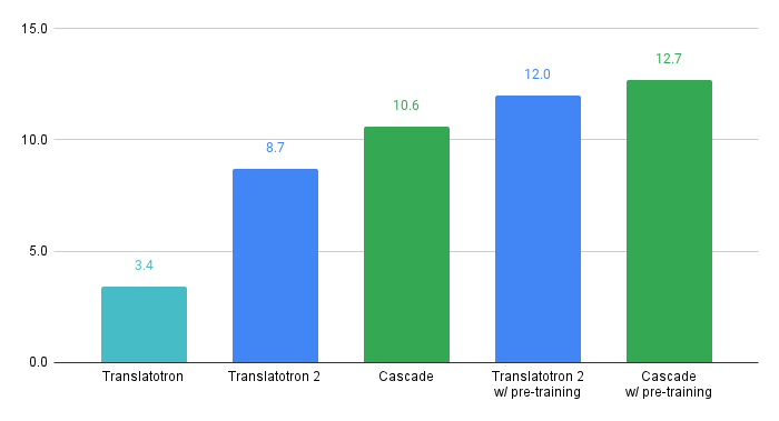
In addition to English NLP tasks, PaLM also shows strong performance on multilingual NLP benchmarks, including translation, even though only 22% of the training corpus is non-English.

We also probe emerging and future capabilities of PaLM on the Beyond the Imitation Game Benchmark (BIG-bench), a recently released suite of more than 150 new language modeling tasks, and find that PaLM achieves breakthrough performance. We compare the performance of PaLM to Gopher and Chinchilla, averaged across a common subset of 58 of these tasks. Interestingly, we note that PaLM’s performance as a function of scale follows a log-linear behavior similar to prior models, suggesting that performance improvements from scale have not yet plateaued. PaLM 540B 5-shot also does better than the average performance of people asked to solve the same tasks.

Scaling behavior of PaLM on a subset of 58 BIG-bench tasks. 

PaLM demonstrates impressive natural language understanding and generation capabilities on several BIG-bench tasks. For example, the model can distinguish cause and effect, understand conceptual combinations in appropriate contexts, and even guess the movie from an emoji.

Examples that showcase PaLM 540B 1-shot performance on BIG-bench tasks: labeling cause and effect, conceptual understanding, guessing movies from emoji, and finding synonyms and counterfactuals.

Reasoning
By combining model scale with chain-of-thought prompting, PaLM shows breakthrough capabilities on reasoning tasks that require multi-step arithmetic or common-sense reasoning. Prior LLMs, like Gopher, saw less benefit from model scale in improving performance.

Standard prompting versus chain-of-thought prompting for an example grade-school math problem. Chain-of-thought prompting decomposes the prompt for a multi-step reasoning problem into intermediate steps (highlighted in yellow), similar to how a person would approach it.

We observed strong performance from PaLM 540B combined with chain-of-thought prompting on three arithmetic datasets and two commonsense reasoning datasets. For example, with 8-shot prompting, PaLM solves 58% of the problems in GSM8K, a benchmark of thousands of challenging grade school level math questions, outperforming the prior top score of 55% achieved by fine-tuning the GPT-3 175B model with a training set of 7500 problems and combining it with an external calculator and verifier.

This new score is especially interesting, as it approaches the 60% average of problems solved by 9-12 year olds, who are the target audience for the question set. We suspect that separate encoding of digits in the PaLM vocabulary helps enable these performance improvements.

Remarkably, PaLM can even generate explicit explanations for scenarios that require a complex combination of multi-step logical inference, world knowledge, and deep language understanding. For example, it can provide high quality explanations for novel jokes not found on the web.

PaLM explains an original joke with two-shot prompts.

Code Generation
LLMs have also been shown [1, 2, 3, 4] to generalize well to coding tasks, such as writing code given a natural language description (text-to-code), translating code from one language to another, and fixing compilation errors (code-to-code).

PaLM 540B shows strong performance across coding tasks and natural language tasks in a single model, even though it has only 5% code in the pre-training dataset. Its few-shot performance is especially remarkable because it is on par with the fine-tuned Codex 12B while using 50 times less Python code for training. This result reinforces earlier findings that larger models can be more sample efficient than smaller models because they better transfer learning from other programming languages and natural language data.

Examples of a fine-tuned PaLM 540B model on text-to-code tasks, such as GSM8K-Python and HumanEval, and code-to-code tasks, such as Transcoder.

We also see a further increase in performance by fine-tuning PaLM on a Python-only code dataset, which we refer to as PaLM-Coder. For an example code repair task called DeepFix, where the objective is to modify initially broken C programs until they compile successfully, PaLM-Coder 540B demonstrates impressive performance, achieving a compile rate of 82.1%, which outperforms the prior 71.7% state of the art. This opens up opportunities for fixing more complex errors that arise during software development.

An example from the DeepFix Code Repair task. The fine-tuned PaLM-Coder 540B fixes compilation errors (left, in red) to a version of code that compiles (right).

Ethical Considerations
Recent research has highlighted various potential risks associated with LLMs trained on web text. It is crucial to analyze and document such potential undesirable risks through transparent artifacts such as model cards and datasheets, which also include information on intended use and testing. To this end, our paper provides a datasheet, model card and Responsible AI benchmark results, and it reports thorough analyses of the dataset and model outputs for biases and risks. While the analysis helps outline some potential risks of the model, domain- and task-specific analysis is essential to truly calibrate, contextualize, and mitigate possible harms. Further understanding of risks and benefits of these models is a topic of ongoing research, together with developing scalable solutions that can put guardrails against malicious uses of language models.

Conclusion and Future Work
PaLM demonstrates the scaling capability of the Pathways system to thousands of accelerator chips across two TPU v4 Pods by training a 540-billion parameter model efficiently with a well-studied, well-established recipe of a dense decoder-only Transformer model. Pushing the limits of model scale enables breakthrough few-shot performance of PaLM across a variety of natural language processing, reasoning, and code tasks.

PaLM paves the way for even more capable models by combining the scaling capabilities with novel architectural choices and training schemes, and brings us closer to the Pathways vision:

“Enable a single AI system to generalize across thousands or millions of tasks, to understand different types of data, and to do so with remarkable efficiency."

Acknowledgements
PaLM is the result of a large, collaborative effort by many teams within Google Research and across Alphabet. We’d like to thank the entire PaLM team for their contributions: Jacob Devlin, Maarten Bosma, Gaurav Mishra, Adam Roberts, Paul Barham, Hyung Won Chung, Charles Sutton, Sebastian Gehrmann, Parker Schuh, Kensen Shi, Sasha Tsvyashchenko, Joshua Maynez, Abhishek Rao, Parker Barnes, Yi Tay, Noam Shazeer, Vinodkumar Prabhakaran, Emily Reif, Nan Du, Ben Hutchinson, Reiner Pope, James Bradbury, Jacob Austin, Michael Isard, Guy Gur-Ari, Pengcheng Yin, Toju Duke, Anselm Levskaya, Sanjay Ghemawat, Sunipa Dev, Henryk Michalewski, Xavier Garcia, Vedant Misra, Kevin Robinson, Liam Fedus, Denny Zhou, Daphne Ippolito, David Luan, Hyeontaek Lim, Barret Zoph, Alexander Spiridonov, Ryan Sepassi, David Dohan, Shivani Agrawal, Mark Omernick, Andrew Dai, Thanumalayan Sankaranarayana Pillai, Marie Pellat, Aitor Lewkowycz, Erica Moreira, Rewon Child, Oleksandr Polozov, Katherine Lee, Zongwei Zhou, Xuezhi Wang, Brennan Saeta, Mark Diaz, Orhan Firat, Michele Catasta, and Jason Wei. PaLM builds on top of work by many, many teams at Google and we would especially like to recognize the T5X team, the Pathways infrastructure team, the JAX team, the Flaxformer team, the XLA team, the Plaque team, the Borg team, and the Datacenter networking infrastructure team. We’d like to thank our co-authors on this blog post, Alexander Spiridonov and Maysam Moussalem, as well as Josh Newlan and Tom Small for the images and animations in this blog post. Finally, we would like to thank our advisors for the project: Noah Fiedel, Slav Petrov, Jeff Dean, Douglas Eck, and Kathy Meier-Hellstern.

Source: Google AI Blog


Introducing CVSS: A Massively Multilingual Speech-to-Speech Translation Corpus

Automatic translation of speech from one language to speech in another language, called speech-to-speech translation (S2ST), is important for breaking down the communication barriers between people speaking different languages. Conventionally, automatic S2ST systems are built with a cascade of automatic speech recognition (ASR), text-to-text machine translation (MT), and text-to-speech (TTS) synthesis sub-systems, so that the system overall is text-centric. Recently, work on S2ST that doesn’t rely on intermediate text representation is emerging, such as end-to-end direct S2ST (e.g., Translatotron) and cascade S2ST based on learned discrete representations of speech (e.g., Tjandra et al.). While early versions of such direct S2ST systems obtained lower translation quality compared to cascade S2ST models, they are gaining traction as they have the potential both to reduce translation latency and compounding errors, and to better preserve paralinguistic and non-linguistic information from the original speech, such as voice, emotion, tone, etc. However, such models usually have to be trained on datasets with paired S2ST data, but the public availability of such corpora is extremely limited.

To foster research on such a new generation of S2ST, we introduce a Common Voice-based Speech-to-Speech translation corpus, or CVSS, which includes sentence-level speech-to-speech translation pairs from 21 languages into English. Unlike existing public corpora, CVSS can be directly used for training such direct S2ST models without any extra processing. In “CVSS Corpus and Massively Multilingual Speech-to-Speech Translation”, we describe the dataset design and development, and demonstrate the effectiveness of the corpus through training of baseline direct and cascade S2ST models and showing performance of a direct S2ST model that approaches that of a cascade S2ST model.

Building CVSS
CVSS is directly derived from the CoVoST 2 speech-to-text (ST) translation corpus, which is further derived from the Common Voice speech corpus. Common Voice is a massively multilingual transcribed speech corpus designed for ASR in which the speech is collected by contributors reading text content from Wikipedia and other text corpora. CoVoST 2 further provides professional text translation for the original transcript from 21 languages into English and from English into 15 languages. CVSS builds on these efforts by providing sentence-level parallel speech-to-speech translation pairs from 21 languages into English (shown in the table below).

To facilitate research with different focuses, two versions of translation speech in English are provided in CVSS, both are synthesized using state-of-the-art TTS systems, with each version providing unique value that doesn’t exist in other public S2ST corpora:

  • CVSS-C: All the translation speech is in a single canonical speaker’s voice. Despite being synthetic, the speech is highly natural, clean, and consistent in speaking style. These properties ease the modeling of the target speech and enable trained models to produce high quality translation speech suitable for general user-facing applications where speech quality is of higher importance than accurately reproducing the speakers' voices.
  • CVSS-T: The translation speech captures the voice from the corresponding source speech. Each S2ST pair has a similar voice on the two sides, despite being in different languages. Because of this, the dataset is suitable for building models where accurate voice preservation is desired, such as for movie dubbing.

Together with the source speech, the two S2ST datasets contain 1,872 and 1,937 hours of speech, respectively.

Source
Language    
Code     Source
  speech (X)  
CVSS-C
  target speech (En)  
CVSS-T
  target speech (En)  
French fr 309.3 200.3 222.3
German de 226.5 137.0 151.2
Catalan ca 174.8 112.1 120.9
Spanish es 157.6 94.3 100.2
Italian it 73.9 46.5 49.2
Persian fa 58.8 29.9 34.5
Russian ru 38.7 26.9 27.4
Chinese zh 26.5 20.5 22.1
Portuguese     pt 20.0 10.4 11.8
Dutch nl 11.2 7.3 7.7
Estonian et 9.0 7.3 7.1
Mongolian mn 8.4 5.1 5.7
Turkish tr 7.9 5.4 5.7
Arabic ar 5.8 2.7 3.1
Latvian lv 4.9 2.6 3.1
Swedish sv 4.3 2.3 2.8
Welsh cy 3.6 1.9 2.0
Tamil ta 3.1 1.7 2.0
Indonesian id 3.0 1.6 1.7
Japanese ja 3.0 1.7 1.8
Slovenian sl 2.9 1.6 1.9
Total 1,153.2 719.1 784.2
Amount of source and target speech of each X-En pair in CVSS (hours).

In addition to translation speech, CVSS also provides normalized translation text matching the pronunciation in the translation speech (on numbers, currencies, acronyms, etc., see data samples below, e.g., where “100%” is normalized as “one hundred percent” or “King George II” is normalized as “king george the second”), which can benefit both model training as well as standardizing the evaluation.

CVSS is released under the Creative Commons Attribution 4.0 International (CC BY 4.0) license and it can be freely downloaded online.

Data Samples

Example 1:
Source audio (French)   
Source transcript (French)    Le genre musical de la chanson est entièrement le disco.
CVSS-C translation audio (English)   
CVSS-T translation audio (English)   
Translation text (English)    The musical genre of the song is 100% Disco.
Normalized translation text (English)        the musical genre of the song is one hundred percent disco
   
   
Example 2:
Source audio (Chinese)       
Source transcript (Chinese)        弗雷德里克王子,英国王室成员,为乔治二世之孙,乔治三世之幼弟。
CVSS-C translation audio (English)       
CVSS-T translation audio (English)       
Translation text (English)        Prince Frederick, member of British Royal Family, Grandson of King George II, brother of King George III.
Normalized translation text (English)        prince frederick member of british royal family grandson of king george the second brother of king george the third

Baseline Models
On each version of CVSS, we trained a baseline cascade S2ST model as well as two baseline direct S2ST models and compared their performance. These baselines can be used for comparison in future research.

Cascade S2ST: To build strong cascade S2ST baselines, we trained an ST model on CoVoST 2, which outperforms the previous states of the art by +5.8 average BLEU on all 21 language pairs (detailed in the paper) when trained on the corpus without using extra data. This ST model is connected to the same TTS models used for constructing CVSS to compose very strong cascade S2ST baselines (ST → TTS).

Direct S2ST: We built two baseline direct S2ST models using Translatotron and Translatotron 2. When trained from scratch with CVSS, the translation quality from Translatotron 2 (8.7 BLEU) approaches that of the strong cascade S2ST baseline (10.6 BLEU). Moreover, when both use pre-training the gap decreases to only 0.7 BLEU on ASR transcribed translation. These results verify the effectiveness of using CVSS to train direct S2ST models.

Translation quality of baseline direct and cascade S2ST models built on CVSS-C, measured by BLEU on ASR transcription from speech translation. The pre-training was done on CoVoST 2 without other extra data sets.

Conclusion
We have released two versions of multilingual-to-English S2ST datasets, CVSS-C and CVSS-T, each with about 1.9K hours of sentence-level parallel S2ST pairs, covering 21 source languages. The translation speech in CVSS-C is in a single canonical speaker’s voice, while the same in CVSS-T is in voices transferred from the source speech. Each of these datasets provides unique value not existing in other public S2ST corpora.

We built baseline multilingual direct S2ST models and cascade S2ST models on both datasets, which can be used for comparison in future works. To build strong cascade S2ST baselines, we trained an ST model on CoVoST 2, which outperforms the previous states of the art by +5.8 average BLEU when trained on the corpus without extra data. Nevertheless, the performance of the direct S2ST models approaches the strong cascade baselines when trained from scratch, and with only 0.7 BLEU difference on ASR transcribed translation when utilized pre-training. We hope this work helps accelerate the research on direct S2ST.

Acknowledgments
We acknowledge the volunteer contributors and the organizers of the Common Voice and LibriVox projects for their contribution and collection of recordings, the creators of Common Voice, CoVoST, CoVoST 2, Librispeech and LibriTTS corpora for their previous work. The direct contributors to the CVSS corpus and the paper include Ye Jia, Michelle Tadmor Ramanovich, Quan Wang, Heiga Zen. We also thank Ankur Bapna, Yiling Huang, Jason Pelecanos, Colin Cherry, Alexis Conneau, Yonghui Wu, Hadar Shemtov and Françoise Beaufays for helpful discussions and support.

Source: Google AI Blog


Detecting Signs of Disease from External Images of the Eye

Three years ago we wrote about our work on predicting a number of cardiovascular risk factors from fundus photos (i.e., photos of the back of the eye)1 using deep learning. That such risk factors could be extracted from fundus photos was a novel discovery and thus a surprising outcome to clinicians and laypersons alike. Since then, we and other researchers have discovered additional novel biomarkers from fundus photos, such as markers for chronic kidney disease and diabetes, and hemoglobin levels to detect anemia.

A unifying goal of work like this is to develop new disease detection or monitoring approaches that are less invasive, more accurate, cheaper and more readily available. However, one restriction to potential broad population-level applicability of efforts to extract biomarkers from fundus photos is getting the fundus photos themselves, which requires specialized imaging equipment and a trained technician.

The eye can be imaged in multiple ways. A common approach for diabetic retinal disease screening is to examine the posterior segment using fundus photographs (left), which have been shown to contain signals of kidney and heart disease, as well as anemia. Another way is to take photographs of the front of the eye (external eye photos; right), which is typically used to track conditions affecting the eyelids, conjunctiva, cornea, and lens.

In “Detection of signs of disease in external photographs of the eyes via deep learning”, in press at Nature Biomedical Engineering, we show that a deep learning model can extract potentially useful biomarkers from external eye photos (i.e., photos of the front of the eye). In particular, for diabetic patients, the model can predict the presence of diabetic retinal disease, elevated HbA1c (a biomarker of diabetic blood sugar control and outcomes), and elevated blood lipids (a biomarker of cardiovascular risk). External eye photos as an imaging modality are particularly interesting because their use may reduce the need for specialized equipment, opening the door to various avenues of improving the accessibility of health screening.

Developing the Model
To develop the model, we used de-identified data from over 145,000 patients from a teleretinal diabetic retinopathy screening program. We trained a convolutional neural network both on these images and on the corresponding ground truth for the variables we wanted the model to predict (i.e., whether the patient has diabetic retinal disease, elevated HbA1c, or elevated lipids) so that the neural network could learn from these examples. After training, the model is able to take external eye photos as input and then output predictions for whether the patient has diabetic retinal disease, or elevated sugars or lipids.

A schematic showing the model generating predictions for an external eye photo.

We measured model performance using the area under the receiver operator characteristic curve (AUC), which quantifies how frequently the model assigns higher scores to patients who are truly positive than patients who are truly negative (i.e., a perfect model scores 100%, compared to 50% for random guesses). The model detected various forms of diabetic retinal disease with AUCs of 71-82%, AUCs of 67-70% for elevated HbA1c, and AUCs of 57-68% for elevated lipids. These results indicate that, though imperfect, external eye photos can help detect and quantify various parameters of systemic health.

Much like the CDC’s pre-diabetes screening questionnaire, external eye photos may be able to help “pre-screen” people and identify those who may benefit from further confirmatory testing. If we sort all patients in our study based on their predicted risk and look at the top 5% of that list, 69% of those patients had HbA1c measurements ≥ 9 (indicating poor blood sugar control for patients with diabetes). For comparison, among patients who are at highest risk according to a risk score based on demographics and years with diabetes, only 55% had HbA1c ≥ 9, and among patients selected at random only 33% had HbA1c ≥ 9.

Assessing Potential Bias
We emphasize that this is promising, yet early, proof-of-concept research showcasing a novel discovery. That said, because we believe that it is important to evaluate potential biases in the data and model, we undertook a multi-pronged approach for bias assessment.

First, we conducted various explainability analyses aimed at discovering what parts of the image contribute most to the algorithm’s predictions (similar to our anemia work). Both saliency analyses (which examine which pixels most influenced the predictions) and ablation experiments (which examine the impact of removing various image regions) indicate that the algorithm is most influenced by the center of the image (the areas of the sclera, iris, and pupil of the eye, but not the eyelids). This is demonstrated below where one can see that the AUC declines much more quickly when image occlusion starts in the center (green lines) than when it starts in the periphery (blue lines).

Explainability analysis shows that (top) all predictions focused on different parts of the eye, and that (bottom) occluding the center of the image (corresponding to parts of the eyeball) has a much greater effect than occluding the periphery (corresponding to the surrounding structures, such as eyelids), as shown by the green line’s steeper decline. The “baseline” is a logistic regression model that takes self-reported age, sex, race and years with diabetes as input.

Second, our development dataset spanned a diverse set of locations within the U.S., encompassing over 300,000 de-identified photos taken at 301 diabetic retinopathy screening sites. Our evaluation datasets comprised over 95,000 images from 198 sites in 18 US states, including datasets of predominantly Hispanic or Latino patients, a dataset of majority Black patients, and a dataset that included patients without diabetes. We conducted extensive subgroup analyses across groups of patients with different demographic and physical characteristics (such as age, sex, race and ethnicity, presence of cataract, pupil size, and even camera type), and controlled for these variables as covariates. The algorithm was more predictive than the baseline in all subgroups after accounting for these factors.

Conclusion
This exciting work demonstrates the feasibility of extracting useful health related signals from external eye photographs, and has potential implications for the large and rapidly growing population of patients with diabetes or other chronic diseases. There is a long way to go to achieve broad applicability, for example understanding what level of image quality is needed, generalizing to patients with and without known chronic diseases, and understanding generalization to images taken with different cameras and under a wider variety of conditions, like lighting and environment. In continued partnership with academic and nonacademic experts, including EyePACS and CGMH, we look forward to further developing and testing our algorithm on larger and more comprehensive datasets, and broadening the set of biomarkers recognized (e.g., for liver disease). Ultimately we are working towards making non-invasive health and wellness tools more accessible to everyone.

Acknowledgements
This work involved the efforts of a multidisciplinary team of software engineers, researchers, clinicians and cross functional contributors. Key contributors to this project include: Boris Babenko, Akinori Mitani, Ilana Traynis, Naho Kitade‎, Preeti Singh, April Y. Maa, Jorge Cuadros, Greg S. Corrado, Lily Peng, Dale R. Webster, Avinash Varadarajan‎, Naama Hammel, and Yun Liu. The authors would also like to acknowledge Huy Doan, Quang Duong, Roy Lee, and the Google Health team for software infrastructure support and data collection. We also thank Tiffany Guo, Mike McConnell, Michael Howell, and Sam Kavusi for their feedback on the manuscript. Last but not least, gratitude goes to the graders who labeled data for the pupil segmentation model, and a special thanks to Tom Small for the ideation and design that inspired the animation used in this blog post.


1The information presented here is research and does not reflect a product that is available for sale. Future availability cannot be guaranteed. 

Source: Google AI Blog


Auto-generated Summaries in Google Docs

For many of us, it can be challenging to keep up with the volume of documents that arrive in our inboxes every day: reports, reviews, briefs, policies and the list goes on. When a new document is received, readers often wish it included a brief summary of the main points in order to effectively prioritize it. However, composing a document summary can be cognitively challenging and time-consuming, especially when a document writer is starting from scratch.

To help with this, we recently announced that Google Docs now automatically generates suggestions to aid document writers in creating content summaries, when they are available. Today we describe how this was enabled using a machine learning (ML) model that comprehends document text and, when confident, generates a 1-2 sentence natural language description of the document content. However, the document writer maintains full control — accepting the suggestion as-is, making necessary edits to better capture the document summary or ignoring the suggestion altogether. Readers can also use this section, along with the outline, to understand and navigate the document at a high level. While all users can add summaries, auto-generated suggestions are currently only available to Google Workspace business customers. Building on grammar suggestions, Smart Compose, and autocorrect, we see this as another valuable step toward improving written communication in the workplace.

A blue summary icon appears in the top left corner when a document summary suggestion is available. Document writers can then view, edit, or ignore the suggested document summary.

Model Details
Automatically generated summaries would not be possible without the tremendous advances in ML for natural language understanding (NLU) and natural language generation (NLG) over the past five years, especially with the introduction of Transformer and Pegasus.

Abstractive text summarization, which combines the individually challenging tasks of long document language understanding and generation, has been a long-standing problem in NLU and NLG research. A popular method for combining NLU and NLG is training an ML model using sequence-to-sequence learning, where the inputs are the document words, and the outputs are the summary words. A neural network then learns to map input tokens to output tokens. Early applications of the sequence-to-sequence paradigm used recurrent neural networks (RNNs) for both the encoder and decoder.

The introduction of Transformers provided a promising alternative to RNNs because Transformers use self-attention to provide better modeling of long input and output dependencies, which is critical in document summarization. Still, these models require large amounts of manually labeled data to train sufficiently, so the advent of Transformers alone was not enough to significantly advance the state-of-the-art in document summarization.

The combination of Transformers with self-supervised pre-training (e.g., BERT, GPT, T5) led to a major breakthrough in many NLU tasks for which limited labeled data is available. In self-supervised pre-training, a model uses large amounts of unlabeled text to learn general language understanding and generation capabilities. Then, in a subsequent fine-tuning stage, the model learns to apply these abilities on a specific task, such as summarization or question answering.

The Pegasus work took this idea one step further, by introducing a pre-training objective customized to abstractive summarization. In Pegasus pre-training, also called Gap Sentence Prediction (GSP), full sentences from unlabeled news articles and web documents are masked from the input and the model is required to reconstruct them, conditioned on the remaining unmasked sentences. In particular, GSP attempts to mask sentences that are considered essential to the document through different heuristics. The intuition is to make the pre-training as close as possible to the summarization task. Pegasus achieved state-of-the-art results on a varied set of summarization datasets. However, a number of challenges remained to apply this research advancement into a product.

Applying Recent Research Advances to Google Docs

  • Data

    Self-supervised pre-training results in an ML model that has general language understanding and generation capabilities, but a subsequent fine-tuning stage is critical for the model to adapt to the application domain. We fine-tuned early versions of our model on a corpus of documents with manually-generated summaries that were consistent with typical use cases.

    However, early versions of this corpus suffered from inconsistencies and high variation because they included many types of documents, as well as many ways to write a summary — e.g., academic abstracts are typically long and detailed, while executive summaries are brief and punchy. This led to a model that was easily confused because it had been trained on so many different types of documents and summaries that it struggled to learn the relationships between any of them.

    Fortunately, one of the key findings in the Pegasus work was that an effective pre-training phase required less supervised data in the fine-tuning stage. Some summarization benchmarks required as few as 1,000 fine-tuning examples for Pegasus to match the performance of Transformer baselines that saw 10,000+ supervised examples — suggesting that one could focus on quality rather than quantity.

    We carefully cleaned and filtered the fine-tuning data to contain training examples that were more consistent and represented a coherent definition of summaries. Despite the fact that we reduced the amount of training data, this led to a higher quality model. The key lesson, consistent with recent work in domains like dataset distillation, was that it was better to have a smaller, high quality dataset, than a larger, high-variance dataset.

  • Serving

    Once we trained the high quality model, we turned to the challenge of serving the model in production. While the Transformer version of the encoder-decoder architecture is the dominant approach to train models for sequence-to-sequence tasks like abstractive summarization, it can be inefficient and impractical to serve in real-world applications. The main inefficiency comes from the Transformer decoder where we generate the output summary token by token through autoregressive decoding. The decoding process becomes noticeably slow when summaries get longer since the decoder attends to all previously generated tokens at each step. RNNs are a more efficient architecture for decoding since there is no self-attention with previous tokens as in a Transformer model.

    We used knowledge distillation, which is the process of transferring knowledge from a large model to a smaller more efficient model, to distill the Pegasus model into a hybrid architecture of a Transformer encoder and an RNN decoder. To improve efficiency we also reduced the number of RNN decoder layers. The resulting model had significant improvements in latency and memory footprint while the quality was still on par with the original model. To further improve the latency and user experience, we serve the summarization model using TPUs, which provide significant speed ups and allow more requests to be handled by a single machine.

Ongoing Challenges and Next Steps
While we are excited by the progress so far, there are a few challenges we are continuing to tackle:

  • Document coverage: Developing a set of documents for the fine-tuning stage was difficult due to the tremendous variety that exists among documents, and the same challenge is true at inference time. Some of the documents our users create (e.g., meeting notes, recipes, lesson plans and resumes) are not suitable for summarization or can be difficult to summarize. Currently, our model only suggests a summary for documents where it is most confident, but we hope to continue broadening this set as our model improves.
  • Evaluation: Abstractive summaries need to capture the essence of a document while being fluent and grammatically correct. A specific document may have many summaries that can be considered correct, and different readers may prefer different ones. This makes it hard to evaluate summaries with automatic metrics only, user feedback and usage statistics will be critical for us to understand and keep improving quality.
  • Long documents: Long documents are some of the toughest documents for the model to summarize because it is harder to capture all the points and abstract them in a single summary, and it can also significantly increase memory usage during training and serving. However, long documents are perhaps most useful for the model to automatically summarize because it can help document writers get a head start on this tedious task. We hope we can apply the latest ML advancements to better address this challenge.

Conclusion
Overall, we are thrilled that we can apply recent progress in NLU and NLG to continue assisting users with reading and writing. We hope the automatic suggestions now offered in Google Workspace make it easier for writers to annotate their documents with summaries, and help readers comprehend and navigate documents more easily.

Acknowledgements
The authors would like to thank the many people across Google that contributed to this work: AJ Motika, Matt Pearson-Beck, Mia Chen, Mahdis Mahdieh, Halit Erdogan, Benjamin Lee, Ali Abdelhadi, Michelle Danoff, Vishnu Sivaji, Sneha Keshav, Aliya Baptista, Karishma Damani, DJ Lick, Yao Zhao, Peter Liu, Aurko Roy, Yonghui Wu, Shubhi Sareen, Andrew Dai, Mekhola Mukherjee, Yinan Wang, Mike Colagrosso, and Behnoosh Hariri. .

Source: Google AI Blog


Offline Optimization for Architecting Hardware Accelerators

Advances in machine learning (ML) often come with advances in hardware and computing systems. For example, the growth of ML-based approaches in solving various problems in vision and language has led to the development of application-specific hardware accelerators (e.g., Google TPUs and Edge TPUs). While promising, standard procedures for designing accelerators customized towards a target application require manual effort to devise a reasonably accurate simulator of hardware, followed by performing many time-intensive simulations to optimize the desired objective (e.g., optimizing for low power usage or latency when running a particular application). This involves identifying the right balance between total amount of compute and memory resources and communication bandwidth under various design constraints, such as the requirement to meet an upper bound on chip area usage and peak power. However, designing accelerators that meet these design constraints is often result in infeasible designs. To address these challenges, we ask: “Is it possible to train an expressive deep neural network model on large amounts of existing accelerator data and then use the learned model to architect future generations of specialized accelerators, eliminating the need for computationally expensive hardware simulations?

In “Data-Driven Offline Optimization for Architecting Hardware Accelerators”, accepted at ICLR 2022, we introduce PRIME, an approach focused on architecting accelerators based on data-driven optimization that only utilizes existing logged data (e.g., data leftover from traditional accelerator design efforts), consisting of accelerator designs and their corresponding performance metrics (e.g., latency, power, etc) to architect hardware accelerators without any further hardware simulation. This alleviates the need to run time-consuming simulations and enables reuse of data from past experiments, even when the set of target applications changes (e.g., an ML model for vision, language, or other objective), and even for unseen but related applications to the training set, in a zero-shot fashion. PRIME can be trained on data from prior simulations, a database of actually fabricated accelerators, and also a database of infeasible or failed accelerator designs1. This approach for architecting accelerators — tailored towards both single- and multi-applications — improves performance upon state-of-the-art simulation-driven methods by about 1.2x-1.5x, while considerably reducing the required total simulation time by 93% and 99%, respectively. PRIME also architects effective accelerators for unseen applications in a zero-shot setting, outperforming simulation-based methods by 1.26x.

PRIME uses logged accelerator data, consisting of both feasible and infeasible accelerators, to train a conservative model, which is used to design accelerators while meeting design constraints. PRIME architects accelerators with up to 1.5x smaller latency, while reducing the required hardware simulation time by up to 99%.

The PRIME Approach for Architecting Accelerators
Perhaps the simplest possible way to use a database of previously designed accelerators for hardware design is to use supervised machine learning to train a prediction model that can predict the performance objective for a given accelerator as input. Then, one could potentially design new accelerators by optimizing the performance output of this learned model with respect to the input accelerator design. Such an approach is known as model-based optimization. However, this simple approach has a key limitation: it assumes that the prediction model can accurately predict the cost for every accelerator that we might encounter during optimization! It is well established that most prediction models trained via supervised learning misclassify adversarial examples that “fool” the learned model into predicting incorrect values. Similarly, it has been shown that even optimizing the output of a supervised model finds adversarial examples that look promising under the learned model2, but perform terribly under the ground truth objective.

To address this limitation, PRIME learns a robust prediction model that is not prone to being fooled by adversarial examples (that we will describe shortly), which would be otherwise found during optimization. One can then simply optimize this model using any standard optimizer to architect simulators. More importantly, unlike prior methods, PRIME can also utilize existing databases of infeasible accelerators to learn what not to design. This is done by augmenting the supervised training of the learned model with additional loss terms that specifically penalize the value of the learned model on the infeasible accelerator designs and adversarial examples during training. This approach resembles a form of adversarial training.

In principle, one of the central benefits of a data-driven approach is that it should enable learning highly expressive and generalist models of the optimization objective that generalize over target applications, while also potentially being effective for new unseen applications for which a designer has never attempted to optimize accelerators. To train PRIME so that it generalizes to unseen applications, we modify the learned model to be conditioned on a context vector that identifies a given neural net application we wish to accelerate (as we discuss in our experiments below, we choose to use high-level features of the target application: such as number of feed-forward layers, number of convolutional layers, total parameters, etc. to serve as the context), and train a single, large model on accelerator data for all applications designers have seen so far. As we will discuss below in our results, this contextual modification of PRIME enables it to optimize accelerators both for multiple, simultaneous applications and new unseen applications in a zero-shot fashion.

Does PRIME Outperform Custom-Engineered Accelerators?
We evaluate PRIME on a variety of actual accelerator design tasks. We start by comparing the optimized accelerator design architected by PRIME targeted towards nine applications to the manually optimized EdgeTPU design. EdgeTPU accelerators are primarily optimized towards running applications in image classification, particularly MobileNetV2, MobileNetV3 and MobileNetEdge. Our goal is to check if PRIME can design an accelerator that attains a lower latency than a baseline EdgeTPU accelerator3, while also constraining the chip area to be under 27 mm2 (the default for the EdgeTPU accelerator). Shown below, we find that PRIME improves latency over EdgeTPU by 2.69x (up to 11.84x in t-RNN Enc), while also reducing the chip area usage by 1.50x (up to 2.28x in MobileNetV3), even though it was never trained to reduce chip area! Even on the MobileNet image-classification models, for which the custom-engineered EdgeTPU accelerator was optimized, PRIME improves latency by 1.85x.

Comparing latencies (lower is better) of accelerator designs suggested by PRIME and EdgeTPU for single-model specialization.
The chip area (lower is better) reduction compared to a baseline EdgeTPU design for single-model specialization.

Designing Accelerators for New and Multiple Applications, Zero-Shot
We now study how PRIME can use logged accelerator data to design accelerators for (1) multiple applications, where we optimize PRIME to design a single accelerator that works well across multiple applications simultaneously, and in a (2) zero-shot setting, where PRIME must generate an accelerator for new unseen application(s) without training on any data from such applications. In both settings, we train the contextual version of PRIME, conditioned on context vectors identifying the target applications and then optimize the learned model to obtain the final accelerator. We find that PRIME outperforms the best simulator-driven approach in both settings, even when very limited data is provided for training for a given application but many applications are available. Specifically in the zero-shot setting, PRIME outperforms the best simulator-driven method we compared to, attaining a reduction of 1.26x in latency. Further, the difference in performance increases as the number of training applications increases.

The average latency (lower is better) of test applications under zero-shot setting compared to a state-of-the-art simulator-driven approach. The text on top of each bar shows the set of training applications.

Closely Analyzing an Accelerator Designed by PRIME
To provide more insight to hardware architecture, we examine the best accelerator designed by PRIME and compare it to the best accelerator found by the simulator-driven approach. We consider the setting where we need to jointly optimize the accelerator for all nine applications, MobileNetEdge, MobileNetV2, MobileNetV3, M4, M5, M64, t-RNN Dec, and t-RNN Enc, and U-Net, under a chip area constraint of 100 mm2. We find that PRIME improves latency by 1.35x over the simulator-driven approach.

Per application latency (lower is better) for the best accelerator design suggested by PRIME and state-of-the-art simulator-driven approach for a multi-task accelerator design. PRIME reduces the average latency across all nine applications by 1.35x over the simulator-driven method.

As shown above, while the latency of the accelerator designed by PRIME for MobileNetEdge, MobileNetV2, MobileNetV3, M4, t-RNN Dec, and t-RNN Enc are better, the accelerator found by the simulation-driven approach yields a lower latency in M5, M6, and U-Net. By closely inspecting the accelerator configurations, we find that PRIME trades compute (64 cores for PRIME vs. 128 cores for the simulator-driven approach) for larger Processing Element (PE) memory size (2,097,152 bytes vs. 1,048,576 bytes). These results show that PRIME favors PE memory size to accommodate the larger memory requirements in t-RNN Dec and t-RNN Enc, where large reductions in latency were possible. Under a fixed area budget, favoring larger on-chip memory comes at the expense of lower compute power in the accelerator. This reduction in the accelerator's compute power leads to higher latency for the models with large numbers of compute operations, namely M5, M6, and U-Net.

Conclusion
The efficacy of PRIME highlights the potential for utilizing the logged offline data in an accelerator design pipeline. A likely avenue for future work is to scale this approach across an array of applications, where we expect to see larger gains because simulator-driven approaches would need to solve a complex optimization problem, akin to searching for needle in a haystack, whereas PRIME can benefit from generalization of the surrogate model. On the other hand, we would also note that PRIME outperforms prior simulator-driven methods we utilize and this makes it a promising candidate to be used within a simulator-driven method. More generally, training a strong offline optimization algorithm on offline datasets of low-performing designs can be a highly effective ingredient in at the very least, kickstarting hardware design, versus throwing out prior data. Finally, given the generality of PRIME, we hope to use it for hardware-software co-design, which exhibits a large search space but plenty of opportunity for generalization. We have also released both the code for training PRIME and the dataset of accelerators.

Acknowledgments
We thank our co-authors Sergey Levine, Kevin Swersky, and Milad Hashemi for their advice, thoughts and suggestions. We thank James Laudon, Cliff Young, Ravi Narayanaswami, Berkin Akin, Sheng-Chun Kao, Samira Khan, Suvinay Subramanian, Stella Aslibekyan, Christof Angermueller, and Olga Wichrowskafor for their help and support, and Sergey Levine for feedback on this blog post. In addition, we would like to extend our gratitude to the members of “Learn to Design Accelerators”, “EdgeTPU”, and the Vizier team for providing invaluable feedback and suggestions. We would also like to thank Tom Small for the animated figure used in this post.


1The infeasible accelerator designs stem from build errors in silicon or compilation/mapping failures. 
2This is akin to adversarial examples in supervised learning – these examples are close to the data points observed in the training dataset, but are misclassified by the classifier. 
3The performance metrics for the baseline EdgeTPU accelerator are extracted from an industry-based hardware simulator tuned to match the performance of the actual hardware. 
4These are proprietary object-detection models, and we refer to them as M4 (indicating Model 4), M5, and M6 in the paper. 

Source: Google AI Blog


Hybrid Quantum Algorithms for Quantum Monte Carlo

The intersection between the computational difficulty and practical importance of quantum chemistry challenges run on quantum computers has long been a focus for Google Quantum AI. We’ve experimentally simulated simple models of chemical bonding, high-temperature superconductivity, nanowires, and even exotic phases of matter such as time crystals on our Sycamore quantum processors. We’ve also developed algorithms suitable for the error-corrected quantum computers we aim to build, including the world’s most efficient algorithm for large-scale quantum computations of chemistry (in the usual way of formulating the problem) and a pioneering approach that allows for us to solve the same problem at an extremely high spatial resolution by encoding the position of the electrons differently.

Despite these successes, it is still more effective to use classical algorithms for studying quantum chemistry than the noisy quantum processors we have available today. However, when the laws of quantum mechanics are translated into programs that a classical computer can run, we often find that the amount of time or memory required scales very poorly with the size of the physical system to simulate.

Today, in collaboration with Dr. Joonho Lee and Professor David Reichmann at Colombia, we present the Nature publication “Unbiasing Fermionic Quantum Monte Carlo with a Quantum Computer”, where we propose and experimentally validate a new way of combining classical and quantum computation to study chemistry, which can replace a computationally-expensive subroutine in a powerful classical algorithm with a “cheaper”, noisy, calculation on a small quantum computer. To evaluate the performance of this hybrid quantum-classical approach, we applied this idea to perform the largest quantum computation of chemistry to date, using 16 qubits to study the forces experienced by two carbon atoms in a diamond crystal. Not only was this experiment four qubits larger than our earlier chemistry calculations on Sycamore, we were also able to use a more comprehensive description of the physics that fully incorporated the interactions between electrons.

Google’s Sycamore quantum processor. Photo Credit: Rocco Ceselin.

A New Way of Combining Quantum and Classical
Our starting point was to use a family of Monte Carlo techniques (projector Monte Carlo, more on that below) to give us a useful description of the lowest energy state of a quantum mechanical system (like the two carbon atoms in a crystal mentioned above). However, even just storing a good description of a quantum state (the “wavefunction”) on a classical computer can be prohibitively expensive, let alone calculating one.

Projector Monte Carlo methods provide a way around this difficulty. Instead of writing down a full description of the state, we design a set of rules for generating a large number of oversimplified descriptions of the state (for example, lists of where each electron might be in space) whose average is a good approximation to the real ground state. The “projector” in projector Monte Carlo refers to how we design these rules — by continuously trying to filter out the incorrect answers using a mathematical process called projection, similar to how a silhouette is a projection of a three-dimensional object onto a two-dimensional surface.

Unfortunately, when it comes to chemistry or materials science, this idea isn’t enough to find the ground state on its own. Electrons belong to a class of particles known as fermions, which have a surprising quantum mechanical quirk to their behavior. When two identical fermions swap places, the quantum mechanical wavefunction (the mathematical description that tells us everything there is to know about them) picks up a minus sign. This minus sign gives rise to the famous Pauli exclusion principle (the fact that two fermions cannot occupy the same state). It can also cause projector Monte Carlo calculations to become inefficient or even break down completely. The usual resolution to this fermion sign problem involves tweaking the Monte Carlo algorithm to include some information from an approximation to the ground state. By using an approximation (even a crude one) to the lowest energy state as a guide, it is usually possible to avoid breakdowns and even obtain accurate estimates of the properties of the true ground state.

Top: An illustration of how the fermion sign problem appears in some cases. Instead of following the blue line curve, our estimates of the energy follow the red curve and become unstable. Bottom: An example of the improvements we might see when we try to fix the sign problem. By using a quantum computer, we hope to improve the initial guess that guides our calculation and obtain a more accurate answer.

For the most challenging problems (such as modeling the breaking of chemical bonds), the computational cost of using an accurate enough initial guess on a classical computer can be too steep to afford, which led our collaborator Dr. Joonho Lee to ask if a quantum computer could help. We had already demonstrated in previous experiments that we can use our quantum computer to approximate the ground state of a quantum system. In these earlier experiments we aimed to measure quantities (such as the energy of the state) that are directly linked to physical properties (like the rate of a chemical reaction). In this new hybrid algorithm, we instead needed to make a very different kind of measurement: quantifying how far the states generated by the Monte Carlo algorithm on our classical computer are from those prepared on the quantum computer. Using some recently developed techniques, we were even able to do all of the measurements on the quantum computer before we ran the Monte Carlo algorithm, separating the quantum computer’s job from the classical computer’s.

A diagram of our calculation. The quantum processor (right) measures information that guides the classical calculation (left). The crosses indicate the qubits, with the ones used for the largest experiment shaded green. The direction of the arrows indicate that the quantum processor doesn’t need any feedback from the classical calculation. The red bars represent the parts of the classical calculation that are filtered out by the data from the quantum computer in order to avoid the fermion sign problem and get a good estimate of properties like the energy of the ground state.

This division of labor between the classical and the quantum computer helped us make good use of both resources. Using our Sycamore quantum processor, we prepared a kind of approximation to the ground state that would be difficult to scale up classically. With a few hours of time on the quantum device, we extracted all of the data we needed to run the Monte Carlo algorithm on the classical computer. Even though the data was noisy (like all present-day quantum computations), it had enough signal that it was able to guide the classical computer towards a very accurate reconstruction of the true ground state (shown in the figure below). In fact, we showed that even when we used a low-resolution approximation to the ground state on the quantum computer (just a few qubits encoding the position of the electrons), the classical computer could efficiently solve a much higher resolution version (with more realism about where the electrons can be).

Top left: a diagram showing the sixteen qubits we used for our largest experiment. Bottom left: an illustration of the carbon atoms in a diamond crystal. Our calculation focused on two atoms (the two that are highlighted in translucent yellow). Right: A plot showing how the error in the total energy (closer to zero is better) changes as we adjust the lattice constant (the spacing between the two carbon atoms). Many properties we might care about, such as the structure of the crystal, can be determined by understanding how the energy varies as we move the atoms around. The calculations we performed using the quantum computer (red points) are comparable in accuracy to two state-of-the-art classical methods (yellow and green triangles) and are extremely close to the numbers we would have gotten if we had a perfect quantum computer rather than a noisy one (black points). The fact that these red and black points are so close tells us that the error in our calculation comes from using an approximate ground state on the quantum computer that was too simple, not from being overwhelmed by noise on the device.

Using our new hybrid quantum algorithm, we performed the largest ever quantum computation of chemistry or materials science. We used sixteen qubits to calculate the energy of two carbon atoms in a diamond crystal. This experiment was four qubits larger than our first chemistry calculations on Sycamore, we obtained more accurate results, and we were able to use a better model of the underlying physics. By guiding a powerful classical Monte Carlo calculation using data from our quantum computer, we performed these calculations in a way that was naturally robust to noise.

We’re optimistic about the promise of this new research direction and excited to tackle the challenge of scaling these kinds of calculations up towards the boundary of what we can do with classical computing, and even to the hard-to-study corners of the universe. We know the road ahead of us is long, but we’re excited to have another tool in our growing toolbox.

Acknowledgements
I’d like to thank my co-authors on the manuscript, Bryan O’Gorman, Nicholas Rubin, David Reichman, Ryan Babbush, and especially Joonho Lee for their many contributions, as well as Charles Neill and Pedram Rousham for their help executing the experiment. I’d also like to thank the larger Google Quantum AI team, who designed, built, programmed, and calibrated the Sycamore processor.

Source: Google AI Blog


Multimodal Bottleneck Transformer (MBT): A New Model for Modality Fusion

People interact with the world through multiple sensory streams (e.g., we see objects, hear sounds, read words, feel textures and taste flavors), combining information and forming associations between senses. As real-world data consists of various signals that co-occur, such as video frames and audio tracks, web images and their captions and instructional videos and speech transcripts, it is natural to apply a similar logic when building and designing multimodal machine learning (ML) models.

Effective multimodal models have wide applications — such as multilingual image retrieval, future action prediction, and vision-language navigation — and are important for several reasons; robustness, which is the ability to perform even when one or more modalities is missing or corrupted, and complementarity between modalities, which is the idea that some information may be present only in one modality (e.g., audio stream) and not in the other (e.g., video frames). While the dominant paradigm for multimodal fusion, called late fusion, consists of using separate models to encode each modality, and then simply combining their output representations at the final step, investigating how to effectively and efficiently combine information from different modalities is still understudied.

In “Attention Bottlenecks for Multimodal Fusion”, published at NeurIPS 2021, we introduce a novel transformer-based model for multimodal fusion in video called Multimodal Bottleneck Transformer (MBT). Our model restricts cross-modal attention flow between latent units in two ways: (1) through tight fusion bottlenecks, that force the model to collect and condense the most relevant inputs in each modality (sharing only necessary information with other modalities), and (2) to later layers of the model, allowing early layers to specialize to information from individual modalities. We demonstrate that this approach achieves state-of-the-art results on video classification tasks, with a 50% reduction in FLOPs compared to a vanilla multimodal transformer model. We have also released our code as a tool for researchers to leverage as they expand on multimodal fusion work.

A Vanilla Multimodal Transformer Model
Transformer models consistently obtain state-of-the-art results in ML tasks, including video (ViViT) and audio classification (AST). Both ViViT and AST are built on the Vision Transformer (ViT); in contrast to standard convolutional approaches that process images pixel-by-pixel, ViT treats an image as a sequence of patch tokens (i.e., tokens from a smaller part, or patch, of an image that is made up of multiple pixels). These models then perform self-attention operations across all pairs of patch tokens. However, using transformers for multimodal fusion is challenging because of their high computational cost, with complexity scaling quadratically with input sequence length.

Because transformers effectively process variable length sequences, the simplest way to extend a unimodal transformer, such as ViT, to the multimodal case is to feed the model a sequence of both visual and auditory tokens, with minimal changes to the transformer architecture. We call this a vanilla multimodal transformer model, which allows free attention flow (called vanilla cross-attention) between different spatial and temporal regions in an image, and across frequency and time in audio inputs, represented by spectrograms. However, while easy to implement by concatenating audio and video input tokens, vanilla cross-attention at all layers of the transformer model is unnecessary because audio and visual inputs contain dense, fine-grained information, which may be redundant for the task — increasing complexity.

Restricting Attention Flow
The issue of growing complexity for long sequences in multimodal models can be mitigated by reducing the attention flow. We restrict attention flow using two methods, specifying the fusion layer and adding attention bottlenecks.

  • Fusion layer (early, mid or late fusion): In multimodal models, the layer where cross-modal interactions are introduced is called the fusion layer. The two extreme versions are early fusion (where all layers in the transformer are cross-modal) and late fusion (where all layers are unimodal and no cross-modal information is exchanged in the transformer encoder). Specifying a fusion layer in between leads to mid fusion. This technique builds on a common paradigm in multimodal learning, which is to restrict cross-modal flow to later layers of the network, allowing early layers to specialize in learning and extracting unimodal patterns.
  • Attention bottlenecks: We also introduce a small set of latent units that form an attention bottleneck (shown below in purple), which force the model, within a given layer, to collate and condense information from each modality before sharing it with the other, while still allowing free attention flow within a modality. We demonstrate that this bottlenecked version (MBT), outperforms or matches its unrestricted counterpart with lower computational cost.
The different attention configurations in our model. Unlike late fusion (top left), where no cross-modal information is exchanged in the transformer encoder, we investigate two pathways for the exchange of cross-modal information. Early and mid fusion (top middle, top right) is done via standard pairwise self attention across all hidden units in a layer. For mid fusion, cross-modal attention is applied only to later layers in the model. Bottleneck fusion (bottom left) restricts attention flow within a layer through tight latent units called attention bottlenecks. Bottleneck mid fusion (bottom right) applies both forms of restriction in conjunction for optimal performance.

Bottlenecks and Computation Cost
We apply MBT to the task of sound classification using the AudioSet dataset and investigate its performance for two approaches: (1) vanilla cross-attention, and (2) bottleneck fusion. For both approaches, mid fusion (shown by the middle values of the x-axis below) outperforms both early (fusion layer = 0) and late fusion (fusion layer = 12). This suggests that the model benefits from restricting cross-modal connections to later layers, allowing earlier layers to specialize in learning unimodal features; however, it still benefits from multiple layers of cross-modal information flow. We find that adding attention bottlenecks (bottleneck fusion) outperforms or maintains performance with vanilla cross-attention for all fusion layers, with more prominent improvements at lower fusion layers.

The impact of using attention bottlenecks for fusion on mAP performance (left) and compute (right) at different fusion layers on AudioSet. Attention bottlenecks (red) improve performance over vanilla cross-attention (blue) at lower computational cost. Mid fusion, which is in fusion layers 4-10, outperforms both early (fusion layer = 0) and late (fusion layer = 12) fusion, with best performance at fusion layer 8.

We compare the amount of computation, measured in GFLOPs, for both vanilla cross-attention and bottleneck fusion. Using a small number of attention bottlenecks (four bottleneck tokens used in our experiments) adds negligible extra computation over a late fusion model, with computation remaining largely constant with varying fusion layers. This is in contrast to vanilla cross-attention, which has a non-negligible computational cost for every layer it is applied to. We note that for early fusion, bottleneck fusion outperforms vanilla cross-attention by over 2 mean average precision points (mAP) on audiovisual sound classification, with less than half the computational cost.

Results on Sound Classification and Action Recognition
MBT outperforms previous research on popular video classification tasks — sound classification (AudioSet and VGGSound) and action recognition (Kinetics and Epic-Kitchens). For multiple datasets, late fusion and MBT with mid fusion (both fusing audio and vision) outperform the best single modality baseline, and MBT with mid fusion outperforms late fusion.

Across multiple datasets, fusing audio and vision outperforms the best single modality baseline, and MBT with mid fusion outperforms late fusion. For each dataset we report the widely used primary metric, i.e., Audioset: mAP, Epic-Kitchens: Top-1 action accuracy, VGGSound, Moments-in-Time and Kinetics: Top-1 classification accuracy.

Visualization of Attention Heatmaps
To understand the behavior of MBT, we visualize the attention computed by our network following the attention rollout technique. We compute heat maps of the attention from the output classification tokens to the image input space for a vanilla cross-attention model and MBT on the AudioSet test set. For each video clip, we show the original middle frame on the left with the ground truth labels overlayed at the bottom. We demonstrate that the attention is particularly focused on regions in the images that contain motion and create sound, e.g., the fingertips on the piano, the sewing machine, and the face of the dog. The fusion bottlenecks in MBT further force the attention to be localized to smaller regions of the images, e.g., the mouth of the dog in the top left and the woman singing in the middle right. This provides some evidence that the tight bottlenecks force MBT to focus only on the image patches that are relevant for an audio classification task and that benefit from mid fusion with audio.

Summary
We introduce MBT, a new transformer-based architecture for multimodal fusion, and explore various fusion approaches using cross-attention between bottleneck tokens. We demonstrate that restricting cross-modal attention via a small set of fusion bottlenecks achieves state-of-the-art results on a number of video classification benchmarks while also reducing computational costs compared to vanilla cross-attention models.

Acknowledgements
This research was conducted by Arsha Nagrani, Anurag Arnab, Shan Yang, Aren Jansen, Cordelia Schmid and Chen Sun. The blog post was written by Arsha Nagrani, Anurag Arnab and Chen Sun. Animations were created by Tom Small.


Source: Google AI Blog


Optimizing Airline Tail Assignments for Cleaner Skies

Airlines around the world are exploring several tactics to meet aggressive CO2 commitments set by the International Civil Aviation Organization (ICAO). This effort has been emphasized in Europe, where aviation accounts for 13.9% of the transportation industry’s carbon emissions. The largest push comes from the European Green Deal, which aims to decrease carbon emissions from transportation by 90% by 2051. The Lufthansa Group has gone even further, committing to a 50% reduction in emissions compared to 2019 by the year 2030 and to reach net-zero emissions by 2050.

One unexpected approach that airlines can use to lower carbon emissions is through optimizing their tail assignment, i.e., how to assign aircraft (identified by the aircraft registration painted on their tails) to legs in a way that minimizes the total operating cost, of which fuel is a major contributor. More fuel needed to operate the aircraft means higher operating costs and more carbon ejected into the atmosphere. For example, a typical long-haul flight (longer than ~4,100km or ~2,500mi) emits about a ton of CO2.

The amount of fuel needed to fly between origin and destination can vary widely — e.g., larger aircraft weigh more and therefore require more fuel, while modern and younger aircraft tend to be more fuel-efficient because they use newer technology. The mass of the fuel itself is also significant. Aircraft are less fuel-efficient early in their flights when their fuel tanks are full than later when the volume of fuel is reduced. Another important factor for the tail assignment is the number of passengers on board; as the number of bookings changes, a smaller or larger aircraft might be required. Other factors can affect fuel consumption, both negative (e.g., headwinds or the age of the engines) or positive (e.g., tailwinds, sharklets, skin).

During the past year, Google’s Operations Research team has been working with the Lufthansa Group to optimize their tail assignment to reduce carbon emissions and the cost of operating their flights. As part of this collaboration, we developed and launched a mathematical tail assignment solver that has been fully integrated to optimize the fleet schedule for SWISS International Air Lines (a Lufthansa Group subsidiary), which we estimate will result in significant reductions in carbon emissions. This solver is the first step of a multi-phase project that started at SWISS.

A Mathematical Model for Tail Assignment
We structure the task of tail assignment optimization as a network flow problem, which is essentially a directed graph characterized by a set of nodes and a set of arcs, with additional constraints related to the problem at hand. Nodes may have either a supply or a demand for a commodity, while arcs have a flow capacity and a cost per unit of flow. The goal is to determine flows for every arc that minimize the total flow cost of each commodity, while maintaining flow balance in the network.

We decided to use a flow network because it is the most common way of modeling this problem in literature, and the commodities, arcs, and nodes of the flow network have a simple one-to-one correspondence to tails, legs, and airports in the real-life problem. In this case, the arcs of the network correspond to each leg of the flight schedule, and each individual tail is a single instance of a commodity that “flows” along the network. Each leg and tail pair in the network has an associated assignment cost, and the model’s objective is to pick valid leg and tail pairs such that these assignment costs are minimized.

A simple example of the tail assignment problem. There are four legs in this schedule and four possible tails that one can assign to those legs. Each tail and leg pair has an associated operational cost. For example, for Leg 1, it costs $50 to assign Tail 1 to it but $100 to assign Tail 2. The optimal solution, with the minimum cost, is to assign Tail 4 to Legs 3 and 2 and Tail 1 to Legs 1 and 4.

Aside from the standard network flow constraints, the model takes into account additional airline-specific constraints so that the solution is tailored to Lufthansa Group airlines. For example, aircraft turnaround times — i.e., the amount of time an aircraft spends on the ground between two consecutive flights — are airline-specific and can vary for a number of reasons. Catering might be loaded at an airline's hub, reducing the turnaround time needed at outstations, or a route could have a higher volume of vacation travelers who often take longer to board and disembark than business travelers. Another constraint is that each aircraft must be on the ground for a nightly check at a specified airport’s maintenance hub to receive mandated maintenance work or cleaning. Furthermore, each airline has their own maintenance schedule, which can require aircraft to undergo routine maintenance checks every few nights, in part to help maintain the aircraft’s fuel efficiency.

Preliminary Results & Next Steps
After using our solver to optimize their fleet schedule in Europe, SWISS Airlines estimates an annual savings of over 3.5 million Swiss Francs and a 6500 ton reduction in CO2 emitted. We expect these savings will multiply when the model is rolled out to the rest of the airlines in the Lufthansa Group and again when traffic returns to pre-COVID levels. Future work will include ensuring this model is usable with larger sets of data, and adding crew and passenger assignment to the optimization system to improve the flight schedules for both passengers and flight crew.

If you are interested in experimenting with your own network flow models, check out OR-Tools, our open source software suite that can be used to build optimization solutions similar to the solver presented in this post. Refer to OR-Tools related documentation for more information.

Acknowledgements
Thanks to Jon Orwant for collaborating extensively on this blog post and for establishing the partnership with Lufthansa and SWISS, along with Alejandra Estanislao. Thanks to the Operations Research Team and to the folks at SWISS, this work could not be possible without their hard work and contributions.

Source: Google AI Blog


Robust Graph Neural Networks

Graph Neural Networks (GNNs) are powerful tools for leveraging graph-structured data in machine learning. Graphs are flexible data structures that can model many different kinds of relationships and have been used in diverse applications like traffic prediction, rumor and fake news detection, modeling disease spread, and understanding why molecules smell.

Graphs can model the relationships between many different types of data, including web pages (left), social connections (center), or molecules (right).

As is standard in machine learning (ML), GNNs assume that training samples are selected uniformly at random (i.e., are an independent and identically distributed or “IID” sample). This is easy to do with standard academic datasets, which are specifically created for research analysis and therefore have every node already labeled. However, in many real world scenarios, data comes without labels, and labeling data can be an onerous process involving skilled human raters, which makes it difficult to label all nodes. In addition, biased training data is a common issue because the act of selecting nodes for labeling is usually not IID. For example, sometimes fixed heuristics are used to select a subset of data (which shares some characteristics) for labeling, and other times, human analysts individually choose data items for labeling using complex domain knowledge.

Localized training data is a typical non-IID bias exhibited in graph-structured data. This is shown on the left figure by taking an orange node and expanding to those around it. Instead, an IID training sample of nodes for labeling would be uniformly distributed, as illustrated by the sampling process on the right.

To quantify the amount of bias present in a training set, one can use methods that measure how large the shift is between two different probability distributions, where the size of the shift can be thought of as the amount of bias. As the shift grows in size, machine learning models have more difficulty generalizing from the biased training set. This situation can meaningfully hurt generalizability — on academic datasets, we’ve observed domain shifts causing a performance drop of 15-20% (as measured by the F1 score).

In “Shift-Robust GNNs: Overcoming the Limitations of Localized Graph Training Data”, presented at NeurIPS 2021, we introduce a solution for using GNNs on biased data. Called Shift-Robust GNN (SR-GNN), this approach is designed to account for distributional differences between biased training data and a graph’s true inference distribution. SR-GNN adapts GNN models to the presence of distributional shift between the nodes labeled for training and the rest of the dataset. We illustrate the effectiveness of SR-GNN in a variety of experiments with biased training datasets on common GNN benchmark datasets for semi-supervised learning and show that SR-GNN outperforms other GNN baselines in accuracy, reducing the negative effects of biased training data by 30–40%.

The Impact of Distribution Shifts on Performance
To demonstrate how distribution shift affects GNN performance, we first generate a number of biased training sets for known academic datasets. Then in order to understand the effect, we plot the generalization (test accuracy) versus a measure of distribution shift (the Central Moment Discrepancy1, CMD). For example, consider the well known PubMed citation dataset, which can be thought of as a graph where the nodes are medical research papers and the edges represent citations between them. When we generate biased training data for PubMed, the plot looks like this:

The effect of distribution shift on the PubMed dataset. Performance (F1) is shown on the y-axis vs. the distribution shift, Central Moment Discrepancy (CMD), on the x-axis, for 100 biased training set samples. As the distribution shift increases, the model’s accuracy falls.

Here one can observe a strong negative correlation between the distribution shift in the dataset and the classification accuracy: as CMD increases, the performance (F1) decreases. That is, GNNs can have difficulty generalizing as their training data looks less like the test dataset.

To address this, we propose a shift-robust regularizer (similar in idea to domain-invariant learning) to minimize the distribution shift between training data and an IID sample from unlabeled data. To do this, we measure the domain shift (e.g., via CMD) in real time as the model is training and apply a direct penalty based on this that forces the model to ignore as much of the training bias as possible. This forces the feature encoders that the model learns for the training data to also work effectively for any unlabeled data, which might come from a different distribution.

The figure below shows what this looks like when compared to a traditional GNN model. We still have the same inputs (the node features X, and the Adjacency Matrix A), and the same number of layers. However at the final embedding Zk from layer (k) of the GNN is compared against embeddings from unlabeled data points to verify that the model is correctly encoding them.

SR-GNN adds two kinds of regularizations to deep GNN models. First, a domain shift regularization (λ term) minimizes the distance between hidden representations of the labeled (Zk) and unlabeled (ZIID) data. Second, the instance weight (β) of the examples can be changed to further approximate the true distribution.

We write this regularization as an additional term in the formula for the model’s loss based on the distance between the training data’s representations and the true data’s distribution (full formulas available in the paper).

In our experiments, we compare our method and a number of standard graph neural network models, to measure their performance on node classification tasks. We demonstrate that adding the SR-GNN regularization gives a 30–40% percent improvement on classification tasks with biased training data labels.

A comparison of SR-GNN using node classification with biased training data on the PubMed dataset. SR-GNN outperforms seven baselines, including DGI, GCN, GAT, SGC and APPNP.

Shift-Robust Regularization for Linear GNNs via Instance Re-weighting
Moreover, it’s worth noting that there’s another class of GNN models (e.g., APPNP, SimpleGCN, etc) that are based on linear operations to speed up their graph convolutions. We also examined how to make these models more reliable in the presence of biased training data. While the same regularization mechanism can not be directly applied due to their different architecture, we can “correct” the training bias by re-weighting the training instances according to their distance from an approximated true distribution. This allows correcting the distribution of the biased training data without passing gradients through the model.

Finally, the two regularizations — for both deep and linear GNNs — can be combined into a generalized regularization for the loss, which combines both domain regularization and instance reweighting (details, including the loss formulas, available in the paper).

Conclusion
Biased training data is common in real world scenarios and can arise due to a variety of reasons, including difficulties of labeling a large amount of data, the various heuristics or inconsistent techniques that are used to choose nodes for labeling, delayed label assignment, and others. We presented a general framework (SR-GNN) that can reduce the influence of biased training data and can be applied to various types of GNNs, including both deeper GNNs and more recent linearized (shallow) versions of these models.

Acknowledgements
Qi Zhu is a PhD Student at UIUC. Thanks to our collaborators Natalia Ponomareva (Google Research) and Jiawei Han (UIUC). Thanks to Tom Small and Anton Tsitsulin for visualizations.


1We note that many measures of distribution shift have been proposed in the literature. Here we use CMD (as it is quick to calculate and generally shows good performance in the domain adaptation literature), but the concept generalizes to any measure of distribution distances/domain shift. 

Source: Google AI Blog