Reddit is one of the world’s largest internet forums, bringing together countless communities looking for entertainment, answers to everyday questions, and so much more.
Recently, the team optimized its Android app to reduce startup speed and improve rendering performance using Baseline Profiles. But the team didn’t stop there. Reddit app developers also enabled Android’s R8 compiler in full mode to maximize bytecode optimization and used Jetpack Compose to rewrite legacy UI, improving both the user and developer experience.
Maximizing optimization using Baseline Profiles and R8 full mode
The Reddit Android app has undergone countless performance upgrades over the years. Reddit developers have long since cleared the list of quick and easy tasks for optimization, but the team still wants to improve the app, bringing its performance to the next level and ensuring it runs well on every Android device.
“Reddit is looking for any strategic improvement to its app performance so we can make the app experience better for new and existing users,” said Rob McWhinnie, a staff engineer at Reddit. “Baseline Profiles fit this use case well since they are based on critical user journeys.”
Reddit’s platform engineering team used screen-specific performance metrics and observability to help its feature teams improve key metrics like time to interactive and scroll performance. Baseline Profiles were a natural fit to help improve these metrics and the user experience behind them, so the team integrated them to make tracking and optimizing easier, using insights from geodata and device classes.
The team built Baseline Profiles for five critical user journeys so far, like scrolling the home feed, logging in, launching the full-screen video player, navigating between subreddits and scrolling their feeds, and using the chat feature.
Simplifying Baseline Profile management in their continuous integration processes, enabled Reddit to remove the need for manual maintenance and streamlining optimization. Now, Baseline Profiles are automatically regenerated for each release.
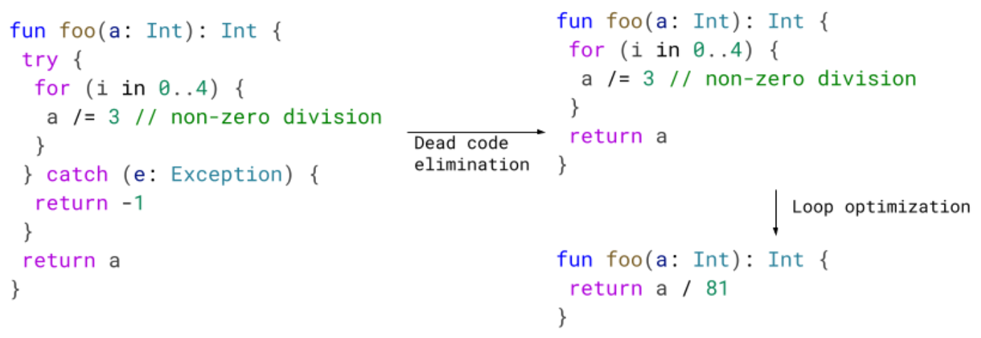
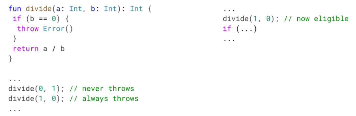
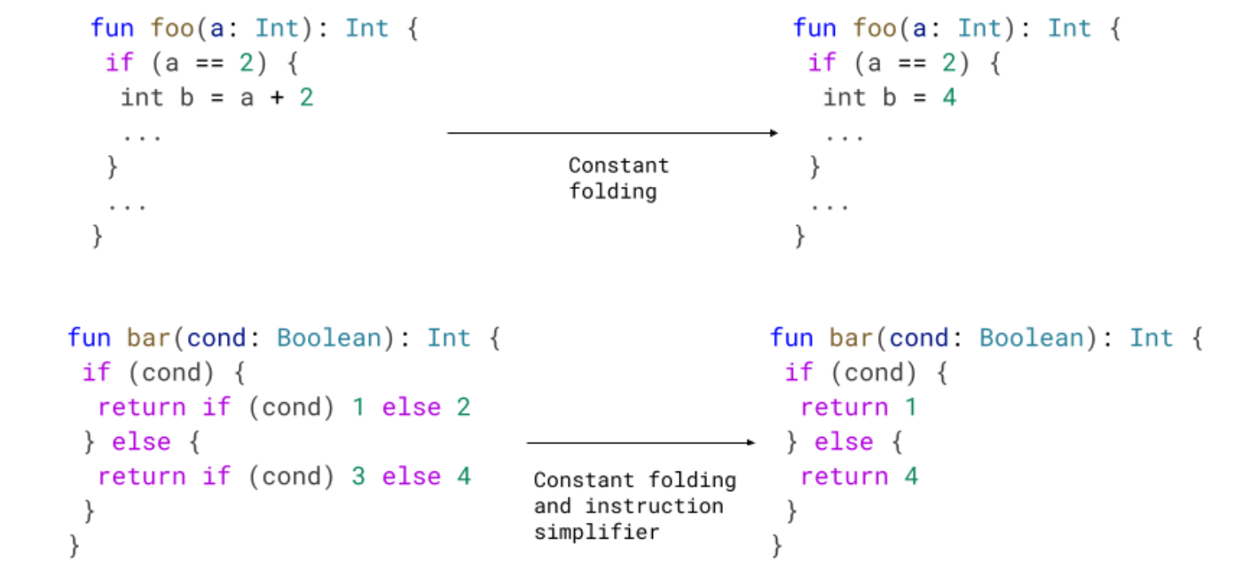
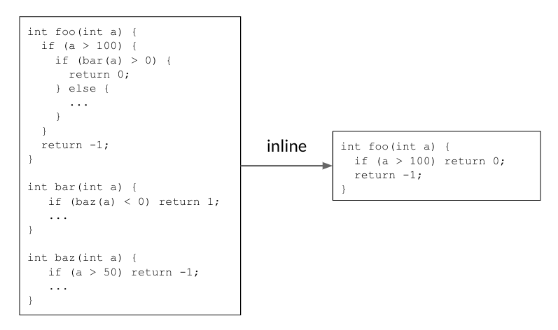
Enabling Android’s R8 optimization compiler in full mode was another area Reddit engineers worked on. The team had already used R8 in compatibility mode, but some of Reddit’s legacy code would’ve made implementing R8’s more aggressive features difficult. The team worked through the app’s existing technical debt first, making it easier to integrate R8's full mode capabilities and maximize Android app optimization.

Improvements with Baseline Profiles and R8 full mode
Reddit's Baseline Profiles and R8 full mode optimization led to multiple performance improvements across the app, with early benchmarks of the first Baseline Profile for feeds showing a 51% median startup time improvement. While responses from Redditors initially confirmed large startup improvements, Baseline Profile optimizations for less frequent journeys, like logging in, saw fewer user reports.
Baseline Profiles for the home feed had a 36% reduction in frozen frames' 95th percentile. Baseline Profiles for the community feed also delivered strong screen load and scroll performance improvements. At the 90th percentile, screen Time To Interactive improved by 12% and time to first draw decreased by 22%. Reddit’s scrolling performance also saw a 12% reduction in P90 slow frames.
The upgrade to R8 full mode led to an increase in Google Play average ratings. The proportion of global positive ratings (fours and fives) increased by four percent, with a notable decrease in negative reports. R8 full mode also reduced total application-not-responding errors by almost 30%.
Overall, the app saw cold start improvements of 20%, scroll performance improvements of 15%, and widespread enhancements in lower-end devices and emerging markets. Google Play vitals saw improvements in slow cold starts, a 10% reduction in excessive frozen frames, and a 30% reduction in excessive slow frames. Nearly 75% of screens, refactored using Jetpack Compose, experienced performance gains.

Further optimizations using Jetpack Compose
Reddit adopted Jetpack Compose years ago and has since rebuilt much of its UI with the toolkit, benefitting both the app and its design system. According to the Reddit team, Google’s ongoing support for Compose’s stability and performance made it a strong fit as Reddit scaled its app, allowing for more efficient feature development and better performance.
One major example is Reddit’s feed rewrite using Compose, which resulted in more maintainable code and an improved developer experience. Compose enabled teams to focus on future work instead of being bogged down by legacy code, allowing them to fix bugs quickly and improve overall app stability.
“The R8 and Compose upgrades were important to deploy in relative isolation and stabilize,” said Drew Heavner, a staff engineer at Reddit. “We feel like we got great outcomes from this work for all teams adopting our modern tech stack and Compose.”
After upgrading to the September 2024 release of Compose, the latest iteration, Reddit saw significant performance gains across the board. Cold start times improved by 13%, excessive slow frames decreased by 25%, and frozen frames dropped by 10%. Low- and mid-tier devices saw even greater improvements where app start times improved by up to 40%, especially in markets with lower-performing devices.
Screens using Reddit’s modern Compose-powered design stack showed substantial improvements in both slow and frozen frame rates. For example, the home feed saw a 23% reduction in frozen frames, and scrolling performance visibly improved according to internal reviews. These updates were well received among users and reflected a 17% increase in the app’s Google Play average rating.

Up-leveling UX through optimization
Adding value to an app isn’t just about introducing new features—it's about refining and optimizing the ones users already love. Investing in performance improvements made Reddit’s key features faster and more reliable, enhancing the overall user experience. These optimizations not only improved app startup and runtime performance but also simplified development workflows, increasing both developer satisfaction and app stability.
The focus on high-traffic features, such as feeds, has demonstrated the power of performance tuning, with substantial gains in user engagement and satisfaction. As the app has become more efficient, both users and developers have benefitted from a cleaner codebase and faster performance.
Looking ahead, Reddit plans to extend the usage of Baseline Profiles to other critical user journeys, including Reddit’s post and comment experiences, ensuring even more users benefit from these ongoing performance improvements.
Reddit’s platform engineers also want to continue collaborating with feature teams to integrate performance improvements across the app. These efforts will ensure that as the app evolves, it remains a smooth, fast, and engaging experience for all Redditors.
“Adding new features isn’t the only way to add value to an experience for users,” said Lauren Darcey, a senior engineering manager at Reddit. “When you find a feature that users love and engage with, taking the time to refine and optimize it can be the difference between a good and a great experience for your users.”
Get started
Improve your app performance using Baseline Profiles, R8 full mode, and Jetpack Compose.


 Posted by Santiago Aboy Solanes - Software Engineer

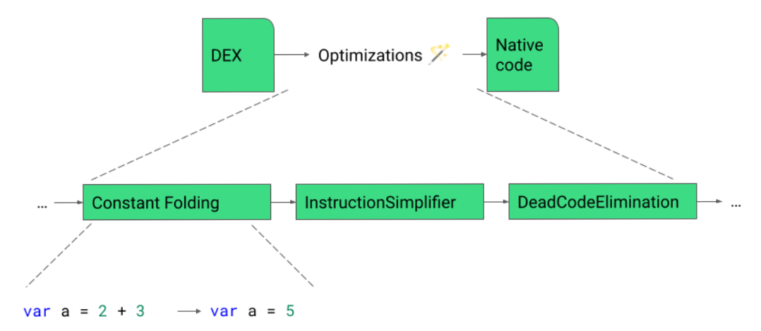
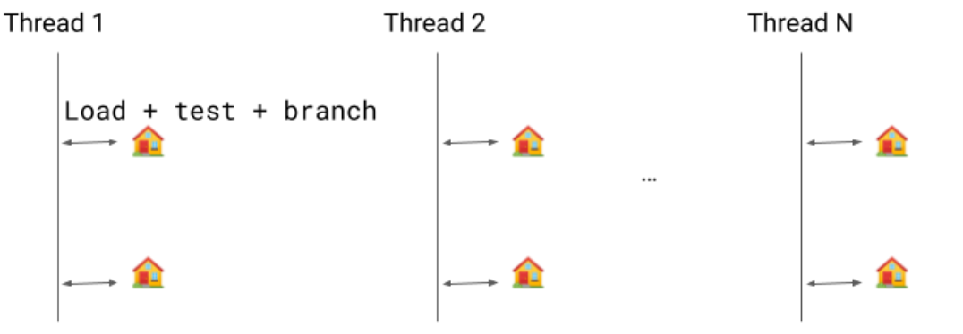
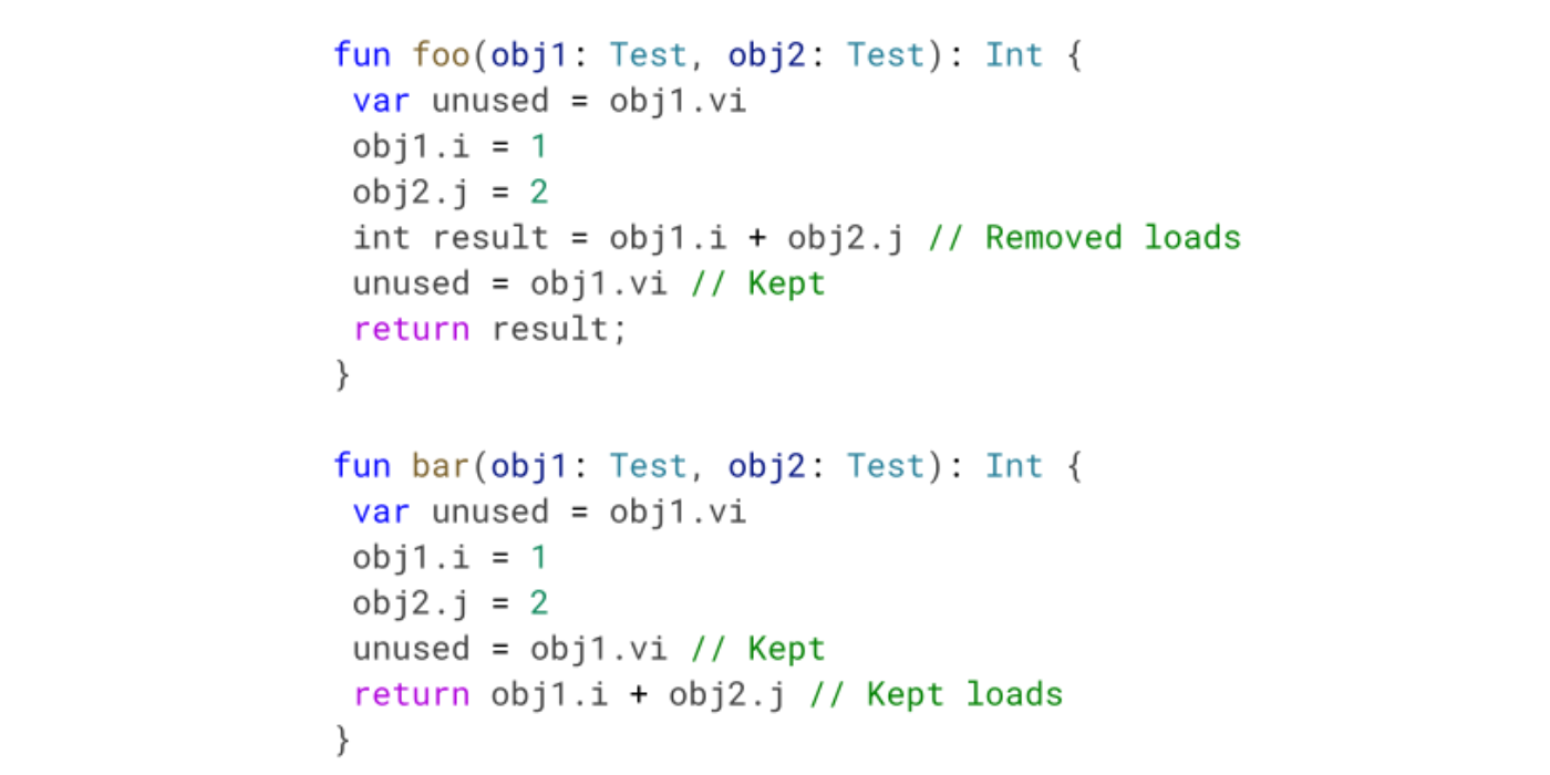
 Previously, we would emit a write barrier for each object modification but we only need a single write barrier because: 1) the mark will be set in
  Implementing this new pass contributes to 0.8% code size reduction.