Tag Archives: Google Brain

Introducing FLAN: More generalizable Language Models with Instruction Fine-Tuning

For a machine learning model to generate meaningful text, it must have a large amount of knowledge about the world as well as the ability to abstract. While language models that are trained to do this are increasingly able to automatically acquire this knowledge as they scale, how to best unlock this knowledge and apply it to specific real-world tasks is not clear.

One well-established technique for doing this is called fine-tuning, which is training a pretrained model such as BERT and T5 on a labeled dataset to adapt it to a downstream task. However, fine-tuning requires a large number of training examples, along with stored model weights for each downstream task, which is not always practical, particularly for large models.

In “Fine-tuned Language Models Are Zero-Shot Learners”, we explore a simple technique called instruction fine-tuning, or instruction tuning for short. This involves fine-tuning a model not to solve a specific task, but to make it more amenable to solving NLP tasks in general. We use instruction tuning to train a model, which we call Fine-tuned LAnguage Net (FLAN). Because the instruction tuning phase of FLAN only takes a small number of updates compared to the large amount of computation involved in pre-training the model, it's the metaphorical dessert to the main course of pretraining. This enables FLAN to perform various unseen tasks.

An illustration of how FLAN works: The model is fine-tuned on disparate sets of instructions and generalizes to unseen instructions. As more types of tasks are added to the fine-tuning data model performance improves.

Background
One recent popular technique for using language models to solve tasks is called zero-shot or few-shot prompting. This technique formulates a task based on text that a language model might have seen during training, where then the language model generates the answer by completing the text. For instance, to classify the sentiment of a movie review, a language model might be given the sentence, “The movie review ‘best RomCom since Pretty Woman’ is _” and be asked to complete the sentence with either the word “positive” or “negative”.

Although this technique demonstrates good performance for some tasks, it requires careful prompt engineering to design tasks to look like data that the model has seen during training — an approach that performs well on some but not all tasks and also can be an unintuitive way for practitioners to interact with the model. For example, the creators of GPT-3 (one of the largest language models in use today) found that such prompting techniques did not result in good performance on natural language inference (NLI) tasks

Instruction Tuning
FLAN instead fine-tunes the model on a large set of varied instructions that use a simple and intuitive description of the task, such as “Classify this movie review as positive or negative,” or “Translate this sentence to Danish.”

Creating a dataset of instructions from scratch to fine-tune the model would take a considerable amount of resources. Therefore, we instead make use of templates to transform existing datasets into an instructional format.

Example templates for a natural language inference dataset.

We show that by training a model on these instructions it not only becomes good at solving the kinds of instructions it has seen during training but becomes good at following instructions in general.

Evaluating the Model
To compare FLAN against other techniques in a meaningful way, we used established benchmark datasets to compare the performance of our model with existing models. Also, we evaluated how FLAN performs without having seen any examples from that dataset during training.

However, if we trained on datasets that were too similar to an evaluation dataset, that might still skew the performance results. For example, training on one question-answering dataset might help the model do better on another question-answering dataset. Because of this, we group all datasets into clusters by type of task and hold out not just the training data for the dataset, but the entire task cluster to which the dataset belongs.

We grouped our datasets into the clusters below.

Results
We evaluated FLAN on 25 tasks and found that it improves over zero-shot prompting on all but four of them. We found that our results are better than zero-shot GPT-3 on 20 of 25 tasks, and better than even few-shot GPT-3 on some tasks.

For various models, we show the average accuracy over all datasets in a task cluster. Natural language inference datasets: ANLI R1–R3, CB, and RTE. Reading comprehension datasets: BoolQ, MultiRC, OpenbookQA. Closed-book QA datasets: ARC, NQ, TriviaQA.

We also find that model scale is very important for the ability of the model to benefit from instruction tuning. At smaller scales, the FLAN technique actually degrades performance, and only at larger scales does the model become able to generalize from instructions in the training data to unseen tasks. This might be because models that are too small do not have enough parameters to perform a large number of tasks.

Instruction tuning only improves performance on unseen tasks for models of certain size.

Conclusion
The FLAN model is not the first to train on a set of instructions, but to our knowledge we are the first to apply this technique at scale and show that it can improve the generalization ability of the model. We hope that the method we presented will help inspire more research into models that can perform unseen tasks and learn from very little data.

We also released the code to perform the transformations so that other researchers can reproduce our results and build on them.

Acknowledgements
We thank our collaborators Vincent Y. Zhao, Kelvin Guu, Adams Wei Yu, Brian Lester, Nan Du, Andrew M. Dai, and Quoc V. Le at Google Research.

Source: Google AI Blog


Learning an Accurate Physics Simulator via Adversarial Reinforcement Learning

Simulation empowers various engineering disciplines to quickly prototype with minimal human effort. In robotics, physics simulations provide a safe and inexpensive virtual playground for robots to acquire physical skills with techniques such as deep reinforcement learning (DRL). However, as the hand-derived physics in simulations does not match the real world exactly, control policies trained entirely within simulation can fail when tested on real hardware — a challenge known as the sim-to-real gap or the domain adaptation problem. The sim-to-real gap for perception-based tasks (such as grasping) has been tackled using RL-CycleGAN and RetinaGAN, but there is still a gap caused by the dynamics of robotic systems. This prompts us to ask, can we learn a more accurate physics simulator from a handful of real robot trajectories? If so, such an improved simulator could be used to refine the robot controller using standard DRL training, so that it succeeds in the real world.

In our ICRA 2021 publication “SimGAN: Hybrid Simulator Identification for Domain Adaptation via Adversarial Reinforcement Learning”, we propose to treat the physics simulator as a learnable component that is trained by DRL with a special reward function that penalizes discrepancies between the trajectories (i.e., the movement of the robots over time) generated in simulation and a small number of trajectories that are collected on real robots. We use generative adversarial networks (GANs) to provide such a reward, and formulate a hybrid simulator that combines learnable neural networks and analytical physics equations, to balance model expressiveness and physical correctness. On robotic locomotion tasks, our method outperforms multiple strong baselines, including domain randomization.

A Learnable Hybrid Simulator
A traditional physics simulator is a program that solves differential equations to simulate the movement or interactions of objects in a virtual world. For this work, it is necessary to build different physical models to represent different environments – if a robot walks on a mattress, the deformation of the mattress needs to be taken into account (e.g., with the finite element method). However, due to the diversity of the scenarios that robots could encounter in the real world, it would be tedious (or even impossible) for such environment-specific modeling techniques, which is why it is useful to instead take an approach based on machine learning. Although simulators can be learned entirely from data, if the training data does not include a wide enough variety of situations, the learned simulator might violate the laws of physics (i.e., deviate from the real-world dynamics) if it needs to simulate situations for which it was not trained. As a result, the robot that is trained in such a limited simulator is more likely to fail in the real world.

To overcome this complication, we construct a hybrid simulator that combines both learnable neural networks and physics equations. Specifically, we replace what are often manually-defined simulator parameters — contact parameters (e.g., friction and restitution coefficients) and motor parameters (e.g., motor gains) — with a learnable simulation parameter function because the unmodeled details of contact and motor dynamics are major causes of the sim-to-real gap. Unlike conventional simulators in which these parameters are treated as constants, in the hybrid simulator they are state-dependent — they can change according to the state of the robot. For example, motors can become weaker at higher speed. These typically unmodeled physical phenomena can be captured using the state-dependent simulation parameter functions. Moreover, while contact and motor parameters are usually difficult to identify and subject to change due to wear-and-tear, our hybrid simulator can learn them automatically from data. For example, rather than having to manually specify the parameters of a robot’s foot against every possible surface it might contact, the simulation learns these parameters from training data.

Comparison between a conventional simulator and our hybrid simulator.

The other part of the hybrid simulator is made up of physics equations that ensure the simulation obeys fundamental laws of physics, such as conservation of energy, making it a closer approximation to the real world and thus reducing the sim-to-real gap.

In our earlier mattress example, the learnable hybrid simulator is able to mimic the contact forces from the mattress. Because the learned contact parameters are state-dependent, the simulator can modulate contact forces based on the distance and velocity of the robot’s feet relative to the mattress, mimicking the effect of the stiffness and damping of a deformable surface. As a result, we do not need to analytically devise a model specifically for deformable surfaces.

Using GANs for Simulator Learning
Successfully learning the simulation parameter functions discussed above would result in a hybrid simulator that can generate similar trajectories to the ones collected on the real robot. The key that enables this learning is defining a metric for the similarity between trajectories. GANs, initially designed to generate synthetic images that share the same distribution, or “style,” with a small number of real images, can be used to generate synthetic trajectories that are indistinguishable from real ones. GANs have two main parts, a generator that learns to generate new instances, and a discriminator that evaluates how similar the new instances are to the training data. In this case, the learnable hybrid simulator serves as the GAN generator, while the GAN discriminator provides the similarity scores.

The GAN discriminator provides the similarity metric that compares the movements of the simulated and the real robot.

Fitting parameters of simulation models to data collected in the real world, a process called system identification (SysID), has been a common practice in many engineering fields. For example, the stiffness parameter of a deformable surface can be identified by measuring the displacements of the surface under different pressures. This process is typically manual and tedious, but using GANs can be much more efficient. For example, SysID often requires a hand-crafted metric for the discrepancy between simulated and real trajectories. With GANs, such a metric is automatically learned by the discriminator. Furthermore, to calculate the discrepancy metric, conventional SysID requires pairing each simulated trajectory to a corresponding real-world one that is generated using the same control policy. Since the GAN discriminator takes only one trajectory as the input and calculates the likelihood that it is collected in the real world, this one-to-one pairing is not needed.

Using Reinforcement Learning (RL) to Learn the Simulator and Refine the Policy
Putting everything together, we formulate simulation learning as an RL problem. A neural network learns the state-dependent contact and motor parameters from a small number of real-world trajectories. The neural network is optimized to minimize the error between the simulated and the real trajectories. Note that it is important to minimize this error over an extended period of time — a simulation that accurately predicts a more distant future will lead to a better control policy. RL is well suited to this because it optimizes the accumulated reward over time, rather than just optimizing a single-step reward.

After the hybrid simulator is learned and becomes more accurate, we use RL again to refine the robot’s control policy within the simulation (e.g., walking across a surface, shown below).

Following the arrows clockwise: (upper left) recording a small number of robot's failed attempts in the target domain (e.g., a real-world proxy in which the leg in red is modified to be much heavier than the source domain); (upper right) learning the hybrid simulator to match trajectories collected in the target domain; (lower right) refining control policies in this learned simulator; (lower left) testing the refined controller directly in the target domain.

Evaluation
Due to limited access to real robots during 2020, we created a second and different simulation (target domain) as a proxy of the real-world. The change of dynamics between the source and the target domains are large enough to approximate different sim-to-real gaps (e.g., making one leg heavier, walking on deformable surfaces instead of hard floor). We assessed whether our hybrid simulator, with no knowledge of these changes, could learn to match the dynamics in the target domain, and if the refined policy in this learned simulator could be successfully deployed in the target domain.

Qualitative results below show that simulation learning with less than 10 minutes of data collected in the target domain (where the floor is deformable) is able to generate a refined policy that performs much better for two robots with different morphologies and dynamics.

Comparison of performance between the initial and refined policy in the target domain (deformable floor) for the hopper and the quadruped robot.

Quantitative results below show that SimGAN outperforms multiple state-of-the-art baselines, including domain randomization (DR) and direct finetuning in target domains (FT).

Comparison of policy performance using different sim-to-real transfer methods in three different target domains for the Quadruped robot: locomotion on deformable surface, with weakened motors, and with heavier bodies.

Conclusion
The sim-to-real gap is one of the key bottlenecks that prevents robots from tapping into the power of reinforcement learning. We tackle this challenge by learning a simulator that can more faithfully model real-world dynamics, while using only a small amount of real-world data. The control policy that is refined in this simulator can be successfully deployed. To achieve this, we augment a classical physics simulator with learnable components, and train this hybrid simulator using adversarial reinforcement learning. To date we have tested its application to locomotion tasks, we hope to build on this general framework by applying it to other robot learning tasks, such as navigation and manipulation.

Source: Google AI Blog


The Importance of A/B Testing in Robotics

Disciplines in the natural sciences, social sciences, and medicine all have to grapple with how to evaluate and compare results within the context of the continually changing real world. In contrast, a significant body of machine learning (ML) research uses a different method that relies on the assumption of a fixed world: measure the performance of a baseline model on fixed data sets, then build a new model aimed at improving on the baseline, and evaluate its performance (on the same fixed data) by comparing its performance to the baseline.

Research into robotics systems and their applications to the real world requires a rethinking of this experiment design. Even in controlled robotic lab environments, it is possible that real-world changes cause the baseline model to perform inconsistently over time, making it unclear whether new models’ performance is an improvement compared to the baseline, or just the result of unintentional, random changes in the experiment setup. As robotics research advances into more complex and challenging real-world scenarios, there is a growing need for both understanding the impact of the ever-changing world on baselines and developing systematic methods to generate informative and clear results.

In this post, we demonstrate how robotics research, even in the relatively controlled environment of a lab, is meaningfully affected by changes in the environment, and discuss how to address this fundamental challenge using random assignment and A/B testing. Although these are classical research methods, they are not generally employed by default in robotics research — yet, they are critical to producing meaningful and measurable scientific results for robotics in real-world scenarios. Additionally, we cover the costs, benefits, and other considerations of using these methods.

The Ever-Changing Real World in Robotics
Even in a robotics lab environment, which is designed to minimize all changes that are not experimental conditions, it is notoriously difficult to set up a perfectly reproducible experiment. Robots get bumped and are subject to wear and tear, lighting changes affect perception, battery charge influences the torque applied to motors — all things that can affect results in ways large and small.

To illustrate this on real robot data, we collected success rate data on one of our simplest setups — moving identical foam dice from one bin to another. For this task, we ran about 33k task trials on two robots over more than five months with the same software and ML model, and took the overall success rate of the last two weeks as baseline. We then measured the historic performance over time in this “very well controlled” environment.

Video of a real robot completing the task: moving identical foam dice from one bin to another.

Given that we did not purposefully change anything during data collection, one would expect the success rate to be statistically similar over time. And yet, this is not what was observed.

The y-axis represents the 95% confidence interval of % change in success rate relative to baseline. If the confidence intervals contain zero, that indicates the success rate is statistically similar to the success rate of baseline. Confidence intervals were computed using Jackknife, with Cochran-Mantel-Haenszel correction to remove operator bias.

Using the sequential data from the plot above, one might conclude that the model ran during weeks 13-14 performed best and that ran during weeks 9-10 performed the worst. One might also expect most, if not all, of the confidence intervals above to contain 0, but only one did. Because no changes were made at any time during these trials, this example effectively demonstrates the impact of unintentional, random real-world changes on even very simple setups. It’s also worth noting that having more trials per experiment wouldn’t remove these differences, instead they will more likely produce a narrower confidence interval making the impact more obvious.

However, what happens when one uses random assignment to compare results, grouping the data randomly rather than sequentially? To answer this, we randomly assigned the above data to the same number of groups for comparison with the baseline. This is equivalent to performing A/B testing where all groups receive the same treatment.

Looking at the chart, we observe that the confidence intervals include zero, indicating success similar to the baseline, as expected.

We performed similar studies with a few other robotics tasks, comparing between sequential and random assignments. They all yielded similar results.

We see that even with no intentional changes, there are statistically significant differences observed for sequential assignment, while random assignment shows the expected result of no statistically significant differences.

Considerations for A/B testing in robotics
While it’s clear based on the above that A/B testing with random assignment is an effective way to control for the unexplainable variance of the real world in robotics, there are some considerations when adopting this approach. Here are several, along with their accompanying pros, cons, and solutions:

  • Absolute vs relative performance: Each experiment needs to be measured against a baseline that is run concurrently. The relative performance metric between baseline and experiment is published with a confidence interval. The absolute performance metric (in baseline or experiment) is less informative, because it depends to an unknown degree on the state of the world when the measurement was taken. However, the statistical differences we’ve measured between the experiment and baseline are sound and robust to reproduction.
  • Data efficiency: With this approach, the baseline always needs to run in parallel with the experimental conditions so they can be compared against each other. Although this may seem wasteful, it is worth the cost when compared against the drawbacks of making an invalid inference against a stale baseline. Furthermore, as the number of random assignment experiments scale up, we can use a single baseline arm with multiple simultaneous experiment arms across independent factors leveraging Google’s overlapping experiment infrastructure. Data efficiency improves with scale.
  • Environmental biases: If there’s any external factor affecting performance overall (lighting, slicker surfaces, etc.), both the baseline and all experiment arms will encounter this factor with similar probability, so its effect will cancel if there’s no relative impact. If there is a correlation between environmental factors and experiment arms, this will show up as differences over time (each environmental factor accumulates in the episodes collected). This can substantially reduce or eliminate the need for effortful environmental resets, and lets us run lifelong experiments and still measure improvements across experimental arms.
  • Human biases: One advantage of random assignment is a reduction in biases introduced by humans. Since human operators cannot know which data sample gets routed to which arm of the experiment, it is harder to have biased experimenters influence any particular outcome.

The Path Forward
The A/B testing experiment framework has been successfully used for a long time in many scientific disciplines to measure performance against changing, unpredictable real-world environments. In this blog post, we show that robotics research can benefit from using this same methodology: it improves the quality and confidence of research results, and avoids the impossible task of perfectly controlling all elements of a fundamentally changing environment. Doing this well requires infrastructure to continuously operate robots, collect data, and tools to make the statistical framework easily accessible to researchers.

Acknowledgements
Arnab Bose, Tuna Toksoz, Yuheng Kuang, Anthony Brohan, Razvan Sudulescu developed the experiment infrastructure and conducted the research. Matthieu Devin suggested the A/A analysis to showcase the differences using existing data. Special thanks to Bill Heavlin, Chris Harris, Vincent Vanhoucke who provided invaluable feedback and support to the work.

Source: Google AI Blog


A New Lens on Understanding Generalization in Deep Learning

Understanding generalization is one of the fundamental unsolved problems in deep learning. Why does optimizing a model on a finite set of training data lead to good performance on a held-out test set? This problem has been studied extensively in machine learning, with a rich history going back more than 50 years. There are now many mathematical tools that help researchers understand generalization in certain models. Unfortunately, most of these existing theories fail when applied to modern deep networks — they are both vacuous and non-predictive in realistic settings. This gap between theory and practice is largest for overparameterized models, which in theory have the capacity to overfit their train sets, but often do not in practice.

In “The Deep Bootstrap Framework: Good Online Learners are Good Offline Generalizers”, accepted at ICLR 2021, we present a new framework for approaching this problem by connecting generalization to the field of online optimization. In a typical setting, a model trains on a finite set of samples, which are reused for multiple epochs. But in online optimization, the model has access to an infinite stream of samples, and can be iteratively updated while processing this stream. In this work, we find that models that train quickly on infinite data are the same models that generalize well if they are instead trained on finite data. This connection brings new perspectives on design choices in practice, and lays a roadmap for understanding generalization from a theoretical perspective.

The Deep Bootstrap Framework
The main idea of the Deep Bootstrap framework is to compare the real world, where there is finite training data, to an "ideal world", where there is infinite data. We define these as:

  • Real World (N, T): Train a model on N train samples from a distribution, for T minibatch stochastic gradient descent (SGD) steps, re-using the same N samples in multiple epochs, as usual. This corresponds to running SGD on the empirical loss (loss on training data), and is the standard training procedure in supervised learning.
  • Ideal World (T): Train the same model for T steps, but use fresh samples from the distribution in each SGD step. That is, we run the exact same training code (same optimizer, learning-rates, batch-size, etc.), but sample a fresh train set in each epoch instead of reusing samples. In this ideal world setting, with an effectively infinite "train set", there is no difference between train error and test error.
Test soft-error for ideal world and real world during SGD iterations for ResNet-18 architecture. We see that the two errors are similar.

A priori, one might expect the real and ideal worlds may have nothing to do with each other, since in the real world the model sees a finite number of examples from the distribution while in the ideal world the model sees the whole distribution. But in practice, we found that the real and ideal models actually have similar test error.

In order to quantify this observation, we simulated an ideal world setting by creating a new dataset, which we call CIFAR-5m. We trained a generative model on CIFAR-10, which we then used to generate ~6 million images. The scale of the dataset was chosen to ensure that it is “virtually infinite” from the model’s perspective, so that the model never resamples the same data. That is, in the ideal world, the model sees an entirely fresh set of samples.

Samples from CIFAR-5m

The figure below presents the test error of several models, comparing their performance when trained on CIFAR-5m data in the real world setting (i.e., re-used data) and the ideal world (“fresh” data). The solid blue line shows a ResNet model in the real world, trained on 50K samples for 100 epochs with standard CIFAR-10 hyperparameters. The dashed blue line shows the corresponding model in the ideal world, trained on 5 million samples in a single pass. Surprisingly, these worlds have very similar test error — the model in some sense "doesn't care" whether it sees re-used samples or fresh ones.

The real world model is trained on 50K samples for 100 epochs, and the ideal world model is trained on 5M samples for a single epoch. The lines show the test error vs. the number of SGD steps.

This also holds for other architectures, e.g., a Multi-Layer-Perceptron (red), a Vision Transformer (green), and across many other settings of architecture, optimizer, data distribution, and sample size. These experiments suggest a new perspective on generalization: models that optimize quickly (on infinite data), generalize well (on finite data). For example, the ResNet model generalizes better than the MLP model on finite data, but this is "because" it optimizes faster even on infinite data.

Understanding Generalization from Optimization Behavior
The key observation is that real world and ideal world models remain close, in test error, for all timesteps, until the real world converges (< 1% train error). Thus, one can study models in the real world by studying their corresponding behavior in the ideal world.

This means that the generalization of the model can be understood in terms of its optimization performance under two frameworks:

  1. Online Optimization: How fast the ideal world test error decreases
  2. Offline Optimization: How fast the real world train error converges

Thus, to study generalization, we can equivalently study the two terms above, which can be conceptually simpler, since they only involve optimization concerns. Based on this observation, good models and training procedures are those that (1) optimize quickly in the ideal world and (2) do not optimize too quickly in the real world.

All design choices in deep learning can be viewed through their effect on these two terms. For example, some advances like convolutions, skip-connections, and pre-training help primarily by accelerating ideal world optimization, while other advances like regularization and data-augmentation help primarily by decelerating real world optimization.

Applying the Deep Bootstrap Framework
Researchers can use the Deep Bootstrap framework to study and guide design choices in deep learning. The principle is: whenever one makes a change that affects generalization in the real world (the architecture, learning-rate, etc.), one should consider its effect on (1) the ideal world optimization of test error (faster is better) and (2) the real world optimization of train error (slower is better).

For example, pre-training is often used in practice to help generalization of models in small-data regimes. However, the reason that pre-training helps remains poorly understood. One can study this using the Deep Bootstrap framework by looking at the effect of pre-training on terms (1) and (2) above. We find that the primary effect of pre-training is to improve the ideal world optimization (1) — pre-training turns the network into a "fast learner" for online optimization. The improved generalization of pretrained models is thus almost exactly captured by their improved optimization in the ideal world. The figure below shows this for Vision-Transformers (ViT) trained on CIFAR-10, comparing training from scratch vs. pre-training on ImageNet.

Effect of pre-training — pre-trained ViTs optimize faster in the ideal world.

One can also study data-augmentation using this framework. Data-augmentation in the ideal world corresponds to augmenting each fresh sample once, as opposed to augmenting the same sample multiple times. This framework implies that good data-augmentations are those that (1) do not significantly harm ideal world optimization (i.e., augmented samples don't look too "out of distribution") or (2) inhibit real world optimization speed (so the real world takes longer to fit its train set).

The main benefit of data-augmentation is through the second term, prolonging the real world optimization time. As for the first term, some aggressive data augmentations (mixup/cutout) can actually harm the ideal world, but this effect is dwarfed by the second term.

Concluding Thoughts
The Deep Bootstrap framework provides a new lens on generalization and empirical phenomena in deep learning. We are excited to see it applied to understand other aspects of deep learning in the future. It is especially interesting that generalization can be characterized via purely optimization considerations, which is in contrast to many prevailing approaches in theory. Crucially, we consider both online and offline optimization, which are individually insufficient, but that together determine generalization.

The Deep Bootstrap framework can also shed light on why deep learning is fairly robust to many design choices: many kinds of architectures, loss functions, optimizers, normalizations, and activation functions can generalize well. This framework suggests a unifying principle: that essentially any choice that works well in the online optimization setting will also generalize well in the offline setting.

Finally, modern neural networks can be either overparameterized (e.g., large networks trained on small data tasks) or underparmeterized (e.g., OpenAI's GPT-3, Google's T5, or Facebook's ResNeXt WSL). The Deep Bootstrap framework implies that online optimization is a crucial factor to success in both regimes.

Acknowledgements
We are thankful to our co-author, Behnam Neyshabur, for his great contributions to the paper and valuable feedback on the blog. We thank Boaz Barak, Chenyang Yuan, and Chiyuan Zhang for helpful comments on the blog and paper.

Source: Google AI Blog


Advancing Semi-supervised Learning with Unsupervised Data Augmentation


Success in deep learning has largely been enabled by key factors such as algorithmic advancements, parallel processing hardware (GPU / TPU), and the availability of large-scale labeled datasets, like ImageNet. However, when labeled data is scarce, it can be difficult to train neural networks to perform well. In this case, one can apply data augmentation methods, e.g., paraphrasing a sentence or rotating an image, to effectively increase the amount of labeled training data. Recently, there has been significant progress in the design of data augmentation approaches for a variety of areas such as natural language processing (NLP), vision, and speech. Unfortunately, data augmentation is often limited to supervised learning only, in which labels are required to transfer from original examples to augmented ones.
Example augmentation operations for text-based (top) or image-based (bottom) training data.
In our recent work, “Unsupervised Data Augmentation (UDA) for Consistency Training”, we demonstrate that one can also perform data augmentation on unlabeled data to significantly improve semi-supervised learning (SSL). Our results support the recent revival of semi-supervised learning, showing that: (1) SSL can match and even outperform purely supervised learning that uses orders of magnitude more labeled data, (2) SSL works well across domains in both text and vision and (3) SSL combines well with transfer learning, e.g., when fine-tuning from BERT. We have also open-sourced our code (github) for the community to replicate and build upon.

Unsupervised Data Augmentation Explained
Unsupervised Data Augmentation (UDA) makes use of both labeled data and unlabeled data. To use labeled data, it computes the loss function using standard methods for supervised learning to train the model, as shown in the left part of the graph below. For unlabeled data, consistency training is applied to enforce the predictions to be similar for an unlabeled example and the augmented unlabeled example, as shown in the right part of the graph. Here, the same model is applied to both the unlabeled example and its augmented counterpart to produce two model predictions, from which a consistency loss is computed (i.e., the distance between the two prediction distributions). UDA then computes the final loss by jointly optimizing both the supervised loss from the labeled data and the unsupervised consistency loss from the unlabeled data.

An overview of Unsupervised Data Augmentation (UDA). Left: Standard supervised loss is computed when labeled data is available. Right: With unlabeled data, a consistency loss is computed between an example and its augmented version.
By minimizing the consistency loss, UDA allows for label information to propagate smoothly from labeled examples to unlabeled ones. Intuitively, one can think of UDA as an implicit iterative process. First, the model relies on a small amount of labeled examples to make correct predictions for some unlabeled examples, from which the label information is propagated to augmented counterparts through the consistency loss. Over time, more and more unlabeled examples will be predicted correctly which reflects the improved generalization of the model. Various other types of noise have been tested for consistency training (e.g., Gaussian noise, adversarial noise, and others), yet we found that data augmentation outperforms all of them, leading to state-of-the-art performance on a wide variety of tasks from language to vision. UDA applies different existing augmentation methods depending on the task at hand, including back translation, AutoAugment, and TF-IDF word replacement.

Benchmarks in NLP and Computer Vision
UDA is surprisingly effective in the low-data regime. With only 20 labeled examples, UDA achieves an error rate of 4.20 on the IMDb sentiment analysis task by leveraging 50,000 unlabeled examples. This result outperforms the previous state-of-the-art model trained on 25,000 labeled examples with an error rate of 4.32. In the large-data regime, with the full training set, UDA also provides robust gains.
Benchmark on IMDb, a sentiment analysis task. UDA surpasses state-of-the-art results in supervised learning across different training sizes.
On the CIFAR-10 semi-supervised learning benchmark, UDA outperforms all existing SSL methods, such as VAT, ICT, and MixMatch by significant margins. With 4k examples, UDA achieves an error rate of 5.27, matching the performance of the fully supervised model that uses 50k examples. Furthermore, with a more advanced architecture, PyramidNet+ShakeDrop, UDA achieves a new state-of-the-art error rate of 2.7, a more than 45% reduction in error rate compared to the previous best semi-supervised result. On SVHN, UDA achieves an error rate of 2.85 with only 250 labeled examples, matching the performance of the fully supervised model trained with ~70k labeled examples.
SSL benchmark on CIFAR-10, an image classification task. UDA surpases all existing semi-supervised learning methods, all of which use the Wide-ResNet-28-2 architecture. At 4000 examples, UDA matches the performance of the fully supervised setting with 50,000 examples.
On ImageNet with 10% labeled examples, UDA improves the top-1 accuracy from 55.1% to 68.7%. In the high-data regime with the fully labeled set and 1.3M extra unlabeled examples, UDA continues to provide gains from 78.3% to 79.0% for top-1 accuracy.

Release
We have released the codebase of UDA, together with all data augmentation methods, e.g., back-translation with pre-trained translation models, to replicate our results. We hope that this release will further advance the progress in semi-supervised learning.

Acknowledgements
Special thanks to the co-authors of the paper Zihang Dai, Eduard Hovy, and Quoc V. Le. We’d also like to thank Hieu Pham, Adams Wei Yu, Zhilin Yang, Colin Raffel, Olga Wichrowska, Ekin Dogus Cubuk, Guokun Lai, Jiateng Xie, Yulun Du, Trieu Trinh, Ran Zhao, Ola Spyra, Brandon Yang, Daiyi Peng, Andrew Dai, Samy Bengio and Jeff Dean for their help with this project. A preprint is available online.

Source: Google AI Blog


Reducing the Need for Labeled Data in Generative Adversarial Networks


Generative adversarial networks (GANs) are a powerful class of deep generative models.The main idea behind GANs is to train two neural networks: the generator, which learns how to synthesise data (such as an image), and the discriminator, which learns how to distinguish real data from the ones synthesised by the generator. This approach has been successfully used for high-fidelity natural image synthesis, improving learned image compression, data augmentation, and more.
Evolution of the generated samples as training progresses on ImageNet. The generator network is conditioned on the class (e.g., "great gray owl" or "golden retriever").
For natural image synthesis, state-of-the-art results are achieved by conditional GANs that, unlike unconditional GANs, use labels (e.g. car, dog, etc.) during training. While this makes the task easier and leads to significant improvements, this approach requires a large amount of labeled data that is rarely available in practice.

In "High-Fidelity Image Generation With Fewer Labels", we propose a new approach to reduce the amount of labeled data required to train state-of-the-art conditional GANs. When combined with recent advancements on large-scale GANs, we match the state-of-the-art in high-fidelity natural image synthesis using 10x fewer labels. Based on this research, we are also releasing a major update to the Compare GAN library, which contains all the components necessary to train and evaluate modern GANs.

Improvements via Semi-supervision and Self-supervision
In conditional GANs, both the generator and discriminator are typically conditioned on class labels. In this work, we propose to replace the hand-annotated ground truth labels with inferred ones. To infer high-quality labels for a large dataset of mostly unlabeled data, we take a two-step approach: First, we learn a feature representation using only the unlabeled portion of the dataset. To learn the feature representations we make use of self-supervision in the form of a recently introduced approach, in which the unlabeled images are randomly rotated and a deep convolutional neural network is tasked with predicting the rotation angle. The idea is that the models need to be able to recognize the main objects and their shapes in order to be successful on this task.
An unlabeled image is randomly rotated and the network is tasked with predicting the rotation angle. Successful models need to capture semantically meaningful image features which can then be used for other vision tasks.
We then consider the activation pattern of one of the intermediate layers of the trained network as the new feature representation of the input, and train a classifier to recognize the label of that input using the labeled portion of the original data set. As the network was pre-trained to extract semantically meaningful features from the data (on the rotation prediction task), training this classifier is more sample-efficient than training the entire network from scratch. Finally, we use this classifier to label the unlabeled data.

To further improve the model quality and training stability we encourage the discriminator network to learn meaningful feature representations which are not forgotten during training by means of an auxiliary loss we introduced previously. These two advancements, combined with large-scale training lead to state-of-the-art conditional GANs for the task of ImageNet synthesis as measured by the Fréchet Inception Distance.
Given a latent vector the generator network produces an image. In each row, linear interpolation between the latent codes of the leftmost and the rightmost image results in a semantic interpolation in the image space.
Compare GAN: A Library for Training and Evaluating GANs
Cutting-edge research on GANs is heavily dependent on a well-engineered and well-tested codebase, since even replicating prior results and techniques requires a significant effort. In order to foster open science and allow the research community benefit from recent advancements, we are releasing a major update of the Compare GAN library. The library includes loss functions, regularization and normalization schemes, neural architectures, and quantitative metrics commonly used in modern GANs, and now supports:
Conclusions and Future Work
Given the growing gap between labeled and unlabeled data sources, it is becoming increasingly important to be able to learn from only partially labeled data. We have shown that a simple yet powerful combination of self-supervision and semi-supervision can help to close this gap for GANs. We believe that self-supervision is a powerful idea that should be investigated for other generative modeling tasks.

Acknowledgments
Work conducted in collaboration with colleagues on the Google Brain team in Zürich, ETH Zürich and UCLA. We would like to thank our paper co-authors Michael Tschannen, Xiaohua Zhai, Olivier Bachem and Sylvain Gelly for their input and feedback. We would like to thank Alexander Kolesnikov, Lucas Beyer and Avital Oliver for helpful discussion on self-supervised learning and semi-supervised learning. We would like to thank Karol Kurach and Marcin Michalski for their major contributions to the Compare GAN library. We would also like to thank Andy Brock, Jeff Donahue and Karen Simonyan for their insights into training GANs on TPUs. The work described in this post also builds upon our work on “Self-Supervised Generative Adversarial Networks” with Ting Chen and Neil Houlsby.

Source: Google AI Blog


Introducing GPipe, an Open Source Library for Efficiently Training Large-scale Neural Network Models


Deep neural networks (DNNs) have advanced many machine learning tasks, including speech recognition, visual recognition, and language processing. Recent advances by BigGan, Bert, and GPT2.0 have shown that ever-larger DNN models lead to better task performance and past progress in visual recognition tasks has also shown a strong correlation between the model size and classification accuracy. For example, the winner of the 2014 ImageNet visual recognition challenge was GoogleNet, which achieved 74.8% top-1 accuracy with 4 million parameters, while just three years later, the winner of the 2017 ImageNet challenge went to Squeeze-and-Excitation Networks, which achieved 82.7% top-1 accuracy with 145.8 million (36x more) parameters. However, in the same period, GPU memory has only increased by a factor of ~3, and the current state-of-the-art image models have already reached the available memory found on Cloud TPUv2s. Hence, there is a strong and pressing need for an efficient, scalable infrastructure that enables large-scale deep learning and overcomes the memory limitation on current accelerators.

Strong correlation between ImageNet accuracy and model size for recently developed representative image classification models
In "GPipe: Efficient Training of Giant Neural Networks using Pipeline Parallelism", we demonstrate the use of pipeline parallelism to scale up DNN training to overcome this limitation. GPipe is a distributed machine learning library that uses synchronous stochastic gradient descent and pipeline parallelism for training, applicable to any DNN that consists of multiple sequential layers. Importantly, GPipe allows researchers to easily deploy more accelerators to train larger models and to scale the performance without tuning hyperparameters. To demonstrate the effectiveness of GPipe, we trained an AmoebaNet-B with 557 million model parameters and input image size of 480 x 480 on Google Cloud TPUv2s. This model performed well on multiple popular datasets, including pushing the single-crop ImageNet accuracy to 84.3%, the CIFAR-10 accuracy to 99%, and the CIFAR-100 accuracy to 91.3%. The core GPipe library has been open sourced under the Lingvo framework.

From Mini- to Micro-Batches
There are two standard ways to speed up moderate-size DNN models. The data parallelism approach employs more machines and splits the input data across them. Another way is to move the model to accelerators, such as GPUs or TPUs, which have special hardware to accelerate model training. However, accelerators have limited memory and limited communication bandwidth with the host machine. Thus, model parallelism is needed for training a bigger DNN model on accelerators by dividing the model into partitions and assigning different partitions to different accelerators. But due to the sequential nature of DNNs, this naive strategy may result in only one accelerator being active during computation, significantly underutilizing accelerator compute capacity. On the other hand, a standard data parallelism approach allows concurrent training of the same model with different input data on multiple accelerators, but cannot increase the maximum model size an accelerator can support.

To enable efficient training across multiple accelerators, GPipe partitions a model across different accelerators and automatically splits a mini-batch of training examples into smaller micro-batches. By pipelining the execution across micro-batches, accelerators can operate in parallel. In addition, gradients are consistently accumulated across micro-batches, so that the number of partitions does not affect the model quality.


Top: The naive model parallelism strategy leads to severe underutilization due to the sequential nature of the network. Only one accelerator is active at a time. Bottom: GPipe divides the input mini-batch into smaller micro-batches, enabling different accelerators to work on separate micro-batches at the same time.
Maximizing Memory and Efficiency
GPipe maximizes memory allocation for model parameters. We ran the experiments on Cloud TPUv2s, each of which has 8 accelerator cores and 64 GB memory (8 GB per accelerator). Without GPipe, a single accelerator can train up to 82 million model parameters due to memory limits. Thanks to recomputation in backpropagation and batch splitting, GPipe reduced intermediate activation memory from 6.26 GB to 3.46GB, enabling 318 million parameters on a single accelerator. We also saw that with pipeline parallelism the maximum model size was proportional to the number of partitions, as expected. With GPipe, AmoebaNet was able to incorporate 1.8 billion parameters on the 8 accelerators of a Cloud TPUv2, 25x times more than is possible without GPipe.

To test efficiency, we measured the effects of GPipe on the model throughput of AmoebaNet-D. Since training required at least two accelerators to fit the model size, we measured the speedup with respect to the naive case with two partitions but no pipeline parallelization. We observed an almost linear speedup in training. Compared to the naive approach with two partitions, distributing the model across four times the accelerators achieved a speedup of 3.5x. While all experiments in our paper used Cloud TPUv2, we see even better performance with the currently available Cloud TPUv3s, each of which has 16 accelerator cores and 256 GB (16 GB per accelerator). GPipe enabled 8 billion parameter Transformer language models on 1024-token sentences with a speedup of 11x when distributing the model across all sixteen accelerators.


Speedup of AmoebaNet-D using GPipe. This model could not fit into one accelerator. The baseline naive-2 is the performance of the native partition approach when the model is split into two partitions. Pipeline-k refers to the performance of GPipe that splits the model into k partitions with k accelerators.
GPipe can also scale training by employing even more accelerators without changes in the hyperparameters. Therefore, it can be combined with data parallelism to scale neural network training using even more accelerators in a complementary way.

Testing Accuracy
We used GPipe to verify the hypothesis that scaling up existing neural networks can achieve even better model quality. We trained an AmoebaNet-B with 557 million model parameters and input image size of 480 x 480 on the ImageNet ILSVRC-2012 dataset. The network was divided into 4 partitions and applied parallel training processes to both model and data. This giant model reached the state-of-the-art 84.3% top-1 / 97% top-5 single-crop validation accuracy without any external data. Large neural networks are not only applicable to datasets like ImageNet, but also relevant for other datasets through transfer learning. It has been shown that better ImageNet models transfer better. We ran transfer learning experiments on the CIFAR10 and CIFAR100 datasets. Our giant models increased the best published CIFAR-10 accuracy to 99% and CIFAR-100 accuracy to 91.3%.

Conclusion
The ongoing development and success of many practical machine learning applications, such as autonomous driving and medical imaging, depend on achieving the highest accuracy possible. As this often requires building larger and even more complex models, we are happy to provide GPipe to the broader research community, and hope it is a useful infrastructure for efficient training of large-scale DNNs.

Acknowledgments
Special thanks to the co-authors of the paper: Youlong Cheng, Dehao Che, HyoukJoong Lee, Jiquan Ngiam, Quoc V. Le, and Zhifeng Chen. We wish to thank Esteban Real, Alok Aggarwal, Xiaodan Song, Naveen Kumar, Mark Heffernan, Rajat Monga, Megan Kacholia, Samy Bengio, and Jeff Dean for their support and valuable input; Noam Shazeer, Patrick Nguyen, Xiaoqiang Zheng, Yonghui Wu, Barret Zoph, Ekin Cubuk, Jonathan Shen, Tianqi Chen, and Vijay Vasudevan for helpful discussions and inspirations; and the larger Google Brain team.

Source: Google AI Blog


Introducing PlaNet: A Deep Planning Network for Reinforcement Learning


Research into how artificial agents can improve their decisions over time is progressing rapidly via reinforcement learning (RL). For this technique, an agent observes a stream of sensory inputs (e.g. camera images) while choosing actions (e.g. motor commands), and sometimes receives a reward for achieving a specified goal. Model-free approaches to RL aim to directly predict good actions from the sensory observations, enabling DeepMind's DQN to play Atari and other agents to control robots. However, this blackbox approach often requires several weeks of simulated interaction to learn through trial and error, limiting its usefulness in practice.

Model-based RL, in contrast, attempts to have agents learn how the world behaves in general. Instead of directly mapping observations to actions, this allows an agent to explicitly plan ahead, to more carefully select actions by "imagining" their long-term outcomes. Model-based approaches have achieved substantial successes, including AlphaGo, which imagines taking sequences of moves on a fictitious board with the known rules of the game. However, to leverage planning in unknown environments (such as controlling a robot given only pixels as input), the agent must learn the rules or dynamics from experience. Because such dynamics models in principle allow for higher efficiency and natural multi-task learning, creating models that are accurate enough for successful planning is a long-standing goal of RL.

To spur progress on this research challenge and in collaboration with DeepMind, we present the Deep Planning Network (PlaNet) agent, which learns a world model from image inputs only and successfully leverages it for planning. PlaNet solves a variety of image-based control tasks, competing with advanced model-free agents in terms of final performance while being 5000% more data efficient on average. We are additionally releasing the source code for the research community to build upon.
The PlaNet agent learning to solve a variety of continuous control tasks from images in 2000 attempts. Previous agents that do not learn a model of the environment often require 50 times as many attempts to reach comparable performance.
How PlaNet Works
In short, PlaNet learns a dynamics model given image inputs and efficiently plans with it to gather new experience. In contrast to previous methods that plan over images, we rely on a compact sequence of hidden or latent states. This is called a latent dynamics model: instead of directly predicting from one image to the next image, we predict the latent state forward. The image and reward at each step is then generated from the corresponding latent state. By compressing the images in this way, the agent can automatically learn more abstract representations, such as positions and velocities of objects, making it easier to predict forward without having to generate images along the way.
Learned Latent Dynamics Model: In a latent dynamics model, the information of the input images is integrated into the hidden states (green) using the encoder network (grey trapezoids). The hidden state is then projected forward in time to predict future images (blue trapezoids) and rewards (blue rectangle).
To learn an accurate latent dynamics model, we introduce:
  • A Recurrent State Space Model: A latent dynamics model with both deterministic and stochastic components, allowing to predict a variety of possible futures as needed for robust planning, while remembering information over many time steps. Our experiments indicate both components to be crucial for high planning performance.
  • A Latent Overshooting Objective: We generalize the standard training objective for latent dynamics models to train multi-step predictions, by enforcing consistency between one-step and multi-step predictions in latent space. This yields a fast and effective objective that improves long-term predictions and is compatible with any latent sequence model.
While predicting future images allows us teach the model, encoding and decoding images (trapezoids in the figure above) requires significant computation, which would slow down planning. However, planning in the compact latent state space is fast since we only need to predict future rewards, and not images, to evaluate an action sequence. For example, the agent can imagine how the position of a ball and its distance to the goal will change for certain actions, without having to visualize the scenario. This allows us to compare 10,000 imagined action sequences with a large batch size every time the agent chooses an action. We then execute the first action of the best sequence found and replan at the next step.
Planning in Latent Space: For planning, we encode past images (gray trapezoid) into the current hidden state (green). From there, we efficiently predict future rewards for multiple action sequences. Note how the expensive image decoder (blue trapezoid) from the previous figure is gone. We then execute the first action of the best sequence found (red box).
Compared to our preceding work on world models, PlaNet works without a policy network -- it chooses actions purely by planning, so it benefits from model improvements on the spot. For the technical details, check out our online research paper or the PDF version.

PlaNet vs. Model-Free Methods
We evaluate PlaNet on continuous control tasks. The agent is only given image observations and rewards. We consider tasks that pose a variety of different challenges:
  • A cartpole swing-up task, with a fixed camera, so the cart can move out of sight. The agent thus must absorb and remember information over multiple frames.
  • A finger spin task that requires predicting two separate objects, as well as the interactions between them.
  • A cheetah running task that includes contacts with the ground that are difficult to predict precisely, calling for a model that can predict multiple possible futures.
  • A cup task, which only provides a sparse reward signal once a ball is caught. This demands accurate predictions far into the future to plan a precise sequence of actions.
  • A walker task, in which a simulated robot starts off by lying on the ground, and must first learn to stand up and then walk.
PlaNet agents trained on a variety of image-based control tasks. The animation shows the input images as the agent is solving the tasks. The tasks pose different challenges: partial observability, contacts with the ground, sparse rewards for catching a ball, and controlling a challenging bipedal robot.
Our work constitutes one of the first examples where planning with a learned model outperforms model-free methods on image-based tasks. The table below compares PlaNet to the well-known A3C agent and the D4PG agent, that combines recent advances in model-free RL. The numbers for these baselines are taken from the DeepMind Control Suite. PlaNet clearly outperforms A3C on all tasks and reaches final performance close to D4PG while, using 5000% less interaction with the environment on average.
One Agent for All Tasks
Additionally, we train a single PlaNet agent to solve all six tasks. The agent is randomly placed into different environments without knowing the task, so it needs to infer the task from its image observations. Without changes to the hyper parameters, the multi-task agent achieves the same mean performance as individual agents. While learning slower on the cartpole tasks, it learns substantially faster and reaches a higher final performance on the challenging walker task that requires exploration.
Video predictions of the PlaNet agent trained on multiple tasks. Holdout episodes collected with the trained agent are shown above and open-loop agent hallucinations below. The agent observes the first 5 frames as context to infer the task and state and accurately predicts ahead for 50 steps given a sequence of actions.
Conclusion
Our results showcase the promise of learning dynamics models for building autonomous RL agents. We advocate for further research that focuses on learning accurate dynamics models on tasks of even higher difficulty, such as 3D environments and real-world robotics tasks. A possible ingredient for scaling up is the processing power of TPUs. We are excited about the possibilities that model-based reinforcement learning opens up, including multi-task learning, hierarchical planning and active exploration using uncertainty estimates.

Acknowledgements
This project is a collaboration with Timothy Lillicrap, Ian Fischer, Ruben Villegas, Honglak Lee, David Ha and James Davidson. We further thank everybody who commented on our paper draft and provided feedback at any point throughout the project.


Source: Google AI Blog


Transformer-XL: Unleashing the Potential of Attention Models


To correctly understand an article, sometimes one will need to refer to a word or a sentence that occurs a few thousand words back. This is an example of long-range dependence — a common phenomenon found in sequential data — that must be understood in order to handle many real-world tasks. While people do this naturally, modeling long-term dependency with neural networks remains a challenge. Gating-based RNNs and the gradient clipping technique improve the ability of modeling long-term dependency, but are still not sufficient to fully address this issue.

One way to approach this challenge is to use Transformers, which allows direct connections between data units, offering the promise of better capturing long-term dependency. However, in language modeling, Transformers are currently implemented with a fixed-length context, i.e. a long text sequence is truncated into fixed-length segments of a few hundred characters, and each segment is processed separately.
Vanilla Transformer with a fixed-length context at training time.
This introduces two critical limitations:
  1. The algorithm is not able to model dependencies that are longer than a fixed length.
  2. The segments usually do not respect the sentence boundaries, resulting in context fragmentation which leads to inefficient optimization. This is particularly troublesome even for short sequences, where long range dependency isn't an issue.
To address these limitations, we propose Transformer-XL a novel architecture that enables natural language understanding beyond a fixed-length context. Transformer-XL consists of two techniques: a segment-level recurrence mechanism and a relative positional encoding scheme.

Segment-level Recurrence
During training, the representations computed for the previous segment are fixed and cached to be reused as an extended context when the model processes the next new segment. This additional connection increases the largest possible dependency length by N times, where N is the depth of the network, because contextual information is now able to flow across segment boundaries. Moreover, this recurrence mechanism also resolves the context fragmentation issue, providing necessary context for tokens in the front of a new segment.
Transformer-XL with segment-level recurrence at training time.
Relative Positional Encodings
Naively applying segment-level recurrence does not work, however, because the positional encodings are not coherent when we reuse the previous segments. For example, consider an old segment with contextual positions [0, 1, 2, 3]. When a new segment is processed, we have positions [0, 1, 2, 3, 0, 1, 2, 3] for the two segments combined, where the semantics of each position id is incoherent through out the sequence. To this end, we propose a novel relative positional encoding scheme to make the recurrence mechanism possible. Moreover, different from other relative positional encoding schemes, our formulation uses fixed embeddings with learnable transformations instead of learnable embeddings, and thus is more generalizable to longer sequences at test time. When both of these approaches are combined, Transformer-XL has a much longer effective context than a vanilla Transformer model at evaluation time.
Vanilla Transformer with a fixed-length context at evaluation time.

Transformer-XL with segment-level recurrence at evaluation time./td>
Furthermore, Transformer-XL is able to process the elements in a new segment all together without recomputation, leading to a significant speed increase (discussed below).

Results
Transformer-XL obtains new state-of-the-art (SoTA) results on a variety of major language modeling (LM) benchmarks, including character-level and word-level tasks on both long and short sequences. Empirically, Transformer-XL enjoys three benefits:
  1. Transformer-XL learns dependency that is about 80% longer than RNNs and 450% longer than vanilla Transformers, which generally have better performance than RNNs, but are not the best for long-range dependency modeling due to fixed-length contexts (please see our paper for details).
  2. Transformer-XL is up to 1,800+ times faster than a vanilla Transformer during evaluation on language modeling tasks, because no re-computation is needed (see figures above).
  3. Transformer-XL has better performance in perplexity (more accurate at predicting a sample) on long sequences because of long-term dependency modeling, and also on short sequences by resolving the context fragmentation problem.
Transformer-XL improves the SoTA bpc/perplexity from 1.06 to 0.99 on enwiki8, from 1.13 to 1.08 on text8, from 20.5 to 18.3 on WikiText-103, from 23.7 to 21.8 on One Billion Word, and from 55.3 to 54.5 on Penn Treebank (without fine tuning). We are the first to break through the 1.0 barrier on char-level LM benchmarks.

We envision many exciting potential applications of Transformer-XL, including but not limited to improving language model pretraining methods such as BERT, generating realistic, long articles, and applications in the image and speech domains, which are also important areas in the world of long-term dependency. For more detail, please see our paper.

The code, pretrained models, and hyperparameters used in our paper are also available in both Tensorflow and PyTorch on GitHub.

Source: Google AI Blog


Curiosity and Procrastination in Reinforcement Learning


Reinforcement learning (RL) is one of the most actively pursued research techniques of machine learning, in which an artificial agent receives a positive reward when it does something right, and negative reward otherwise. This carrot-and-stick approach is simple and universal, and allowed DeepMind to teach the DQN algorithm to play vintage Atari games and AlphaGoZero to play the ancient game of Go. This is also how OpenAI taught its OpenAI-Five algorithm to play the modern video game Dota, and how Google taught robotic arms to grasp new objects. However, despite the successes of RL, there are many challenges to making it an effective technique.

Standard RL algorithms struggle with environments where feedback to the agent is sparse — crucially, such environments are common in the real world. As an example, imagine trying to learn how to find your favorite cheese in a large maze-like supermarket. You search and search but the cheese section is nowhere to be found. If at every step you receive no “carrot” and no “stick”, there’s no way to tell if you are headed in the right direction or not. In the absence of rewards, what is to stop you from wandering around in circles? Nothing, except perhaps your curiosity, which motivates you go into a product section that looks unfamiliar to you in pursuit of your sought-after cheese.

In “Episodic Curiosity through Reachability” — the result of a collaboration between the Google Brain team, DeepMind and ETH Zürich — we propose a novel episodic memory-based model of granting RL rewards, akin to curiosity, which leads to exploring the environment. Since we want the agent not only to explore the environment but also to solve the original task, we add a reward bonus provided by our model to the original sparse task reward. The combined reward is not sparse anymore which allows standard RL algorithms to learn from it. Thus, our curiosity method expands the set of tasks which are solvable with RL.
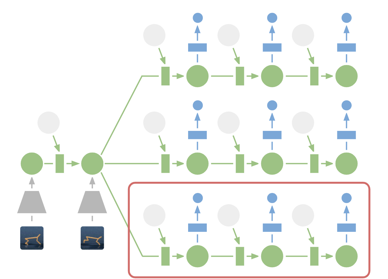
Episodic Curiosity through Reachability: Observations are added to memory, reward is computed based on how far the current observation is from the most similar observation in memory. The agent receives more reward for seeing observations which are not yet represented in memory.
The key idea of our method is to store the agent's observations of the environment in an episodic memory, while also rewarding the agent for reaching observations not yet represented in memory. Being “not in memory” is the definition of novelty in our method — seeking such observations means seeking the unfamiliar. Such a drive to seek the unfamiliar will lead the artificial agent to new locations, thus keeping it from wandering in circles and ultimately help it stumble on the goal. As we will discuss later, our formulation can save the agent from undesired behaviours which some other formulations are prone to. Much to our surprise, those behaviours bear some similarity to what a layperson would call “procrastination”.

Previous Curiosity Formulations
While there have been many attempts to formulate curiosity in the past[1][2][3][4], in this post we  focus on one natural and very popular approach: curiosity through prediction-based surprise, explored in the recent paper “Curiosity-driven Exploration by Self-supervised Prediction” (commonly referred to as the ICM method). To illustrate how surprise leads to curiosity, again consider our analogy of looking for cheese in a supermarket.
Illustration © Indira Pasko, used under CC BY-NC-ND 4.0 license.
As you wander throughout the market, you try to predict the future (“Now I’m in the meat section, so I think the section around the corner is the fish section — those are usually adjacent in this supermarket chain”). If your prediction is wrong, you are surprised (“No, it’s actually the vegetables section. I didn’t expect that!”) and thus rewarded. This makes you more motivated to look around the corner in the future, exploring new locations just to see if your expectations about them meet the reality (and, hopefully, stumble upon the cheese).

Similarly, the ICM method builds a predictive model of the dynamics of the world and gives the agent rewards when the model fails to make good predictions — a marker of surprise or novelty. Note that exploring unvisited locations is not directly a part of the ICM curiosity formulation. For the ICM method, visiting them is only a way to obtain more “surprise” and thus maximize overall rewards. As it turns out, in some environments there could be other ways to inflict self-surprise, leading to unforeseen results.
Agent imbued with surprise-based curiosity gets stuck when it encounters TV. GIF adopted from a video by © Deepak Pathak, used under CC BY 2.0 license.
The Dangers of “Procrastination”
In "Large-Scale Study of Curiosity-Driven Learning", the authors of the ICM method along with researchers from OpenAI show a hidden danger of surprise maximization: agents can learn to indulge procrastination-like behaviour instead of doing something useful for the task at hand. To see why, consider a common thought experiment the authors call the “noisy TV problem”, in which an agent is put into a maze and tasked with finding a highly rewarding item (akin to “cheese” in our previous supermarket example). The environment also contains a TV for which the agent has the remote control. There is a limited number of channels (each with a distinct show) and every press on the remote control switches to a random channel. How would an agent perform in such an environment?

For the surprise-based curiosity formulation, changing channels would result in a large reward, as each change is unpredictable and surprising. Crucially, even after cycling through all the available channels, the random channel selection ensures every new change will still be surprising — the agent is making predictions about what will be on the TV after a channel change, and will very likely be wrong, leading to surprise. Importantly, even if the agent has already seen every show on every channel, the change is still unpredictable. Because of this, the agent imbued with surprise-based curiosity would eventually stay in front of the TV forever instead of searching for a highly rewarding item — akin to procrastination. So, what would be a definition of curiosity which does not lead to such behaviour?

Episodic Curiosity
In “Episodic Curiosity through Reachability”, we explore an episodic memory-based curiosity model that turns out to be less prone to “self-indulging” instant gratification. Why so? Using our example above, after changing channels for a while, all of the shows will end up in memory. Thus, the TV won’t be so attractive anymore: even if the order of shows appearing on the screen is random and unpredictable, all those shows are already in memory! This is the main difference to the surprise-based methods: our method doesn’t even try to make bets about the future which could be hard (or even impossible) to predict. Instead, the agent examines the past to know if it has seen observations similar to the current one. Thus our agent won’t be drawn that much to the instant gratification provided by the noisy TV. It will have to go and explore the world outside of the TV to get more reward.

But how do we decide whether the agent is seeing the same thing as an existing memory? Checking for an exact match could be meaningless: in a realistic environment, the agent rarely sees exactly the same thing twice. For example, even if the agent returned to exactly the same room, it would still see this room under a different angle compared to its memories.

Instead of checking for an exact match in memory, we use a deep neural network that is trained to measure how similar two experiences are. To train this network, we have it guess whether two observations were experienced close together in time, or far apart in time. Temporal proximity is a good proxy for whether two experiences should be judged to be part of the same experience. This training leads to a general concept of novelty via reachability which is illustrated below.
Graph of reachabilities would determine novelty. In practice, this graph is not available — so we train a neural network approximator to estimate a number of steps between observations.
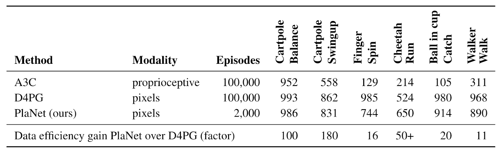
Experimental Results
To compare the performance of different approaches to curiosity, we tested them in two visually rich 3D environments: ViZDoom and DMLab. In those environments, the agent was tasked with various problems like searching for a goal in a maze or collecting good and avoiding bad objects. The DMLab environment happens to provide the agent with a laser-like science fiction gadget. The standard setting in the previous work on DMLab was to equip the agent with this gadget for all tasks, and if the agent does not need a gadget for a particular task, it is free not to use it. Interestingly, similar to the noisy TV experiment described above, the surprise-based ICM method actually uses this gadget a lot even when it is useless for the task at hand! When tasked with searching for a high-rewarding item in the maze, it instead prefers to spend time tagging walls because this yields a lot of “surprise” reward. Theoretically, predicting the result of tagging should be possible, but in practice is too hard as it apparently requires a deeper knowledge of physics than is available to a standard agent.
Surprise-based ICM method is persistently tagging the wall instead of exploring the maze.
Our method instead learns reasonable exploration behaviour under the same conditions. This is because it does not try to predict the result of its actions, but rather seeks observations which are “harder” to achieve from those already in the episodic memory. In other words, the agent implicitly pursues goals which require more effort to reach from memory than just a single tagging action.
Our method shows reasonable exploration.
It is interesting to see that our approach to granting reward penalizes an agent running in circles. This is because after completing the first circle the agent does not encounter new observations other than those in memory, and thus receives no reward:
Our reward visualization: red means negative reward, green means positive reward. Left to right: map with rewards, map with locations currently in memory, first-person view.
At the same time, our method favors good exploration behavior:
Our reward visualization: red means negative reward, green means positive reward. Left to right: map with rewards, map with locations currently in memory, first-person view.
We hope that our work will help lead to a new wave of exploration methods, going beyond surprise and learning more intelligent exploration behaviours. For an in-depth analysis of our method, please take a look at the preprint of our research paper.

Acknowledgements:
This project is a result of a collaboration between the Google Brain team, DeepMind and ETH Zürich. The core team includes Nikolay Savinov, Anton Raichuk, Raphaël Marinier, Damien Vincent, Marc Pollefeys, Timothy Lillicrap and Sylvain Gelly. We would like to thank Olivier Pietquin, Carlos Riquelme, Charles Blundell and Sergey Levine for the discussions about the paper. We are grateful to Indira Pasko for the help with illustrations.

References:
[1] "Count-Based Exploration with Neural Density Models", Georg Ostrovski, Marc G. Bellemare, Aaron van den Oord, Remi Munos
[2] "#Exploration: A Study of Count-Based Exploration for Deep Reinforcement Learning", Haoran Tang, Rein Houthooft, Davis Foote, Adam Stooke, Xi Chen, Yan Duan, John Schulman, Filip De Turck, Pieter Abbeel
[3] "Unsupervised Learning of Goal Spaces for Intrinsically Motivated Goal Exploration", Alexandre Péré, Sébastien Forestier, Olivier Sigaud, Pierre-Yves Oudeyer
[4] "VIME: Variational Information Maximizing Exploration", Rein Houthooft, Xi Chen, Yan Duan, John Schulman, Filip De Turck, Pieter Abbeel

Source: Google AI Blog