Author Archives: Google AI Blog

Using Deep Learning to Improve Usability on Mobile Devices


Tapping is the most commonly used gesture on mobile interfaces, and is used to trigger all kinds of actions ranging from launching an app to entering text. While the style of clickable elements (e.g., buttons) in traditional desktop graphical user interfaces is often conventionally defined, on mobile interfaces it can still be difficult for people to distinguish tappable versus non-tappable elements due to the diversity of styles. This confusion can lead to false affordances (e.g., a feature that could be mistaken for a button) and a lack of discoverability that can lead to user frustration, uncertainty, and errors. To avoid this, interface designers can conduct a study or a visual affordance test to help clarify the tappability of items in their interfaces. However, such studies are time-consuming and their findings are often limited to a specific app or interface design.

In our CHI'19 paper, "Modeling Mobile Interface Tappability Using Crowdsourcing and Deep Learning", we introduced an approach for modeling the usability of mobile interfaces at scale. We crowdsourced a task to study UI elements across a range of mobile apps to measure the perceived tappability by a user. Our model predictions were consistent with the user group at the ~90% level, demonstrating that a machine learning model can be effectively used to estimate the perceived tappability of interface elements in their design without the need for expensive and time consuming user testing.
Predicting Tappability with Deep Learning
Designers often use visual properties such as the color or depth of an element to signify its availability for interaction on interfaces, e.g., the blue color and underline of a link. While these common signifiers are useful, it is not always clear when to apply them in each specific design setting. Furthermore, with design trends evolving, traditional signifiers are constantly being altered and challenged, potentially causing user uncertainty and mistakes.

To understand how users perceive this changing landscape, we analyzed the potential signifiers affecting tappability in real mobile apps—element type (e.g., check boxes, text boxes, etc.), location, size, color, and words. We started by crowdsourcing volunteers to label the perceived clickability of ~20,000 unique interface elements from ~3,500 apps. With the exception of text boxes, type signifiers yielded low uncertainty in user perceived tappability. The location signifier refers to the position of a feature on the screen and is informed by the common layout design in mobile apps, as demonstrated in the figure below.
Heatmaps displaying the accuracy of tappable and non-tappable elements by location, where warmer colors represent areas of higher accuracy. Users labeled non-tappable elements more accurately towards the upper center of the interface, and tappable elements towards the bottom center of the interface.
The impact of element size was relatively weak, but did indicate confusion in the case of large non-tappable elements. Users showed a tendency to bright colors and short word counts for tappable elements, though word semantics also played a significant role.

We used these labels to train a simple deep neural network that predicts the likelihood that a user will perceive an interface element as tappable versus non-tappable. For a given element of the interface, the model uses a range of features, including the spatial context of the element on the screen (location), the semantics and functionality of the element (words and type), and the visual appearance (size as well as raw pixels). The neural network model applies a convolutional neural network (CNN) to extract features from raw pixels, and uses learned semantic embeddings to represent text content and element properties. The concatenation of all these features are then fed to a fully-connected network layer, the output of which produces a binary classification of an element's tappability.

Evaluation of the Model
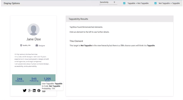
The model allowed us to automatically diagnose mismatches between the tappability of each interface element as perceived by a user—predicted by our model—and the intended or actual tappable state of the element specified by the developer or designer. In the example below, our model predicts that there is a 73% chance that a user would think the labels such as "Followers" or "Following" are tappable, while these interface elements are in fact not programmed to be tappable.
To understand how our model behaves compared to human users, particularly when there is ambiguity in human perception, we generated a second, independent dataset by crowdsourcing an effort among 290 volunteers to label each of 2,000 unique interface elements with respect to their perceived tappability. Each element was labeled independently by five different users. We found that more than 40% of the elements in our sample were labeled inconsistently by volunteers. Our model matches this uncertainty in human perception quite well, as demonstrated in the figure below.
The scatterplot of the tappability probability predicted by the model (the Y axis) versus the consistency in the human user labels (the X axis) for each element in the consistency dataset.
When users agree an element's tappability, our model tends to give a more definite answer—a probability close to 1 for tappable and close to 0 for not tappable. When workers are less consistent on an element (towards the middle of the X axis), our model is also less certain about the decision. Overall, our model achieved reasonable accuracy of matching human perception in identifying tappable UI elements with a mean precision of 90.2% and recall of 87.0%.

Predicting tappability is merely one example of what we can do with machine learning to solve usability issues in user interfaces. There are many other challenges in interaction design and user experience research where deep learning models can offer a vehicle to distill large, diverse user experience datasets and advance scientific understandings about interaction behaviors.

Acknowledgements
This research was a joint work of Amanda Swangson, summer intern at Google, and Yang Li, a Research Scientist in Deep Learning and Human Computer Interaction.

Source: Google AI Blog


Unifying Physics and Deep Learning with TossingBot


Though considerable progress has been made in enabling robots to grasp objects efficiently, visually self adapt or even learn from real-world experiences, robotic operations still require careful consideration in how they pick up, handle, and place various objects -- especially in unstructured settings. Consider for example, this picking robot which took 1st place in the stowing task of the Amazon Robotics Challenge:
It's an impressive system, built with many design features that kinematically prevent it from dropping objects due to unforeseen dynamics: from its steady and deliberate movements, to its gripper fingers that mechanically constrain the momentum of the object so that it doesn't slip.

This robot, like many others, is designed to tolerate the dynamics of the unstructured world. But instead of just tolerating dynamics, can robots learn to use them advantageously, developing an "intuition" of physics that would allow them to complete tasks more efficiently? Perhaps in doing so, robots can improve their capabilities and acquire complex athletic skills like tossing, sliding, spinning, swinging, or catching, potentially leading to many useful applications, such as more efficient debris clearing robots in disaster response scenarios -- where time is of the essence.

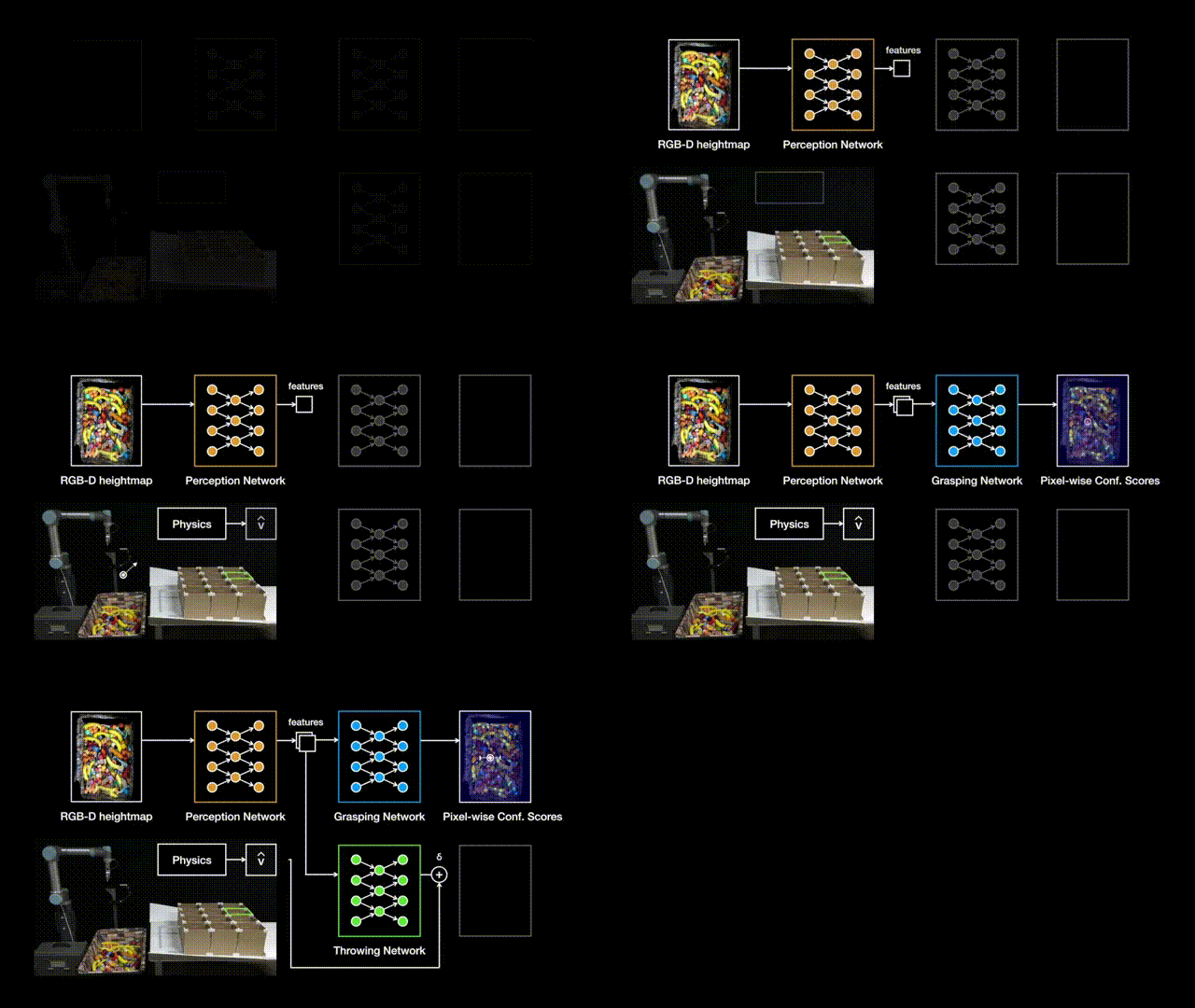
To explore this concept, we worked with researchers at Princeton, Columbia, and MIT to develop TossingBot: a picking robot for our real, random world that learns to grasp and throw objects into selected boxes outside its natural range. We find that by learning to throw, TossingBot is capable of achieving picking speeds that are twice as fast as previous systems, with twice the effective placing range. TossingBot jointly learns grasping and throwing policies using an end-to-end neural network that maps from visual observations (RGB-D images) to control parameters for motion primitives. Using overhead cameras to track where objects land, TossingBot improves itself over time through self-supervision. More technical details are available in an early preprint on arXiv.
The Challenges
Throwing is a particularly difficult task as it depends on many factors: from how the object is picked up (i.e., "pre-throw conditions"), to the object's physical properties like mass, friction, aerodynamics, etc. For example, if you grasp a screwdriver by the handle near the center of mass and throw it, it would land much closer than if you had grasped it from the metal tip, which would swing forward and land much farther away. Regardless of how you grasped it though, tossing a screwdriver is incredibly different from tossing a ping pong ball, which would land closer due to air resistance. Manually designing a solution that explicitly handles these factors for every random object is nearly impossible.
Throwing depends on many factors: from how you picked it up, to object properties and dynamics.
Through deep learning, however, our robots can learn from experience rather than rely on manual case-by-case engineering. Previously we've shown that our robots can learn to push and grasp a large variety of objects, but accurately throwing objects requires a larger understanding of projectile physics. Acquiring this knowledge from scratch with only trial-and-error is not only time consuming and expensive, but also generally doesn't work outside of very specific, and carefully set up training scenarios.

Unifying Physics and Deep Learning
A fundamental component of TossingBot is that it learns to throw by integrating simple physics and deep learning, which enables it to train quickly and generalize to new scenarios. Physics provides prior models of how the world works, and we can leverage these models to develop initial controllers for our robots. In the case of throwing, for example, we can use projectile ballistics to provide an estimate for the throwing velocity that is needed to get an object to land at a target location. We can then use neural networks to predict adjustments on top of that estimate from physics, in order to compensate for unknown dynamics as well as the noise and variability of the real world. We call this hybrid formulation Residual Physics, and it enables TossingBot to achieve throwing accuracies of 85%.
At the start of training with randomly initialized weights, TossingBot repeatedly attempts bad grasps. Over time, however, TossingBot learns better ways to grasp objects and simultaneously improves its ability to throw. Occasionally the robot randomly explores what happens if it throws an object at a velocity that it hasn't tried before. When the bin is emptied, TossingBot lifts the boxes to allow objects to slide back into the bin. This way, human intervention is kept at a minimum during training. By 10,000 grasp and throw attempts (or 14 hours of training time), it is capable of achieving throwing accuracies of 85%, with a grasping reliability of 87% in clutter.
TossingBot starts out performing poorly (left), but progressively learns to grasp and toss overnight (right).
Generalizing to New Scenarios
By integrating physics and deep learning, TossingBot is capable of rapidly adapting to never-before-seen throwing locations and objects. For example, after training on objects with simple shapes like wooden blocks, balls, and markers, it can perform reasonably well on new objects such as fake fruit, decorative items, and office objects. On new objects, TossingBot starts out with lower performance, but quickly adapts within a few hundred training steps (i.e., an hour or two) to achieve similar performance as with training objects. We've found that combining physics and deep learning with Residual Physics yields better performance than baseline alternatives (e.g. deep learning without physics). We even tried this task ourselves, and we were pleasantly surprised to learn that TossingBot is more accurate than any of us engineers! Though take that with a grain of salt, as we've yet to test TossingBot against anyone with any actual athletic talent.
TossingBot can generalize to new objects, and is more accurate at throwing than the average Googler.
We also test our policies on their ability to generalize to new target locations previously unseen in training. To this end, we train on a set of boxes, then later test on a different set of boxes with entirely different landing areas. In this setting, we find that Residual Physics for throwing helps significantly, since the initial estimates of throwing velocities from projectile ballistics easily generalize to new target locations, while the residuals help make adjustments on top of those estimates to compensate for varying object properties in the real world. This is in contrast to the baseline alternative of using deep learning without physics, which can only handle target locations seen during training.
TossingBot uses Residual Physics to throw objects to unforeseen locations.
Emerging Semantics from Interaction
To explore what TossingBot learns, we place several objects in the bin, capture images, and feed them into TossingBot's trained neural network to extract intermediate pixel-wise deep features. By clustering these features based on similarity and visualizing nearest neighbors as a heatmap (hotter regions indicate more similarity in feature space), we can localize all ping pong balls in the scene. Even though the orange block shares a similar color with the ping pong balls, its features are different enough for TossingBot to make a distinction. Likewise, we can also use the extracted features to localize all marker pens, which share similar shape and mass, but do not share color. These observations suggest that TossingBot likely learns to rely more on geometric cues (e.g. shape) to learn grasping and throwing. It is also possible that the learned features reflect second-order attributes such as physical properties, which can influence how the objects should be thrown.
TossingBot learns deep features that distinguish object categories without explicit supervision.
These emerging features were learned implicitly from scratch without any explicit supervision beyond task-level grasping and throwing. Yet, they seem to be sufficient for enabling the system to distinguish between object categories (i.e., ping pong balls and marker pens). As such, this experiment speaks out to a broader concept related to machine vision: how should robots learn the semantics of the visual world? From the perspective of classic computer vision, semantics are often pre-defined using human-fabricated image datasets and manually constructed class categories. However, our experiment suggests that it is possible to implicitly learn such object-level semantics from physical interactions alone, as long as they matter for the task at hand. The more complex these interactions, the higher the resolution of the semantics. Towards more generally intelligent robots -- perhaps it is sufficient for them to develop their own notion of semantics through interaction, without requiring any human intervention.

Limitations and Future Work
Although TossingBot's results are promising, it does have its limitations. For example, it assumes that objects are robust enough to withstand landing collisions after being thrown -- further work is required to learn throws that account for fragile objects, or possibly train other robots to catch objects in ways that cushion the landing. Furthermore, TossingBot infers control parameters only from visual data -- exploring additional senses (e.g. force-torque or tactile) may enable the system to better react to new objects.

The combination of physics and deep learning that made TossingBot possible naturally leads to an interesting question: what else could benefit from Residual Physics? Investigating how the idea generalizes to other types of tasks and interactions is a promising direction for future research.

You can learn more about this work in the summary video below.
Acknowledgements
This research was done by Andy Zeng, Shuran Song (faculty at Columbia University), Johnny Lee, Alberto Rodriguez (faculty at MIT), and Thomas Funkhouser (faculty at Princeton University), with special thanks to Ryan Hickman for valuable managerial support, Ivan Krasin and Stefan Welker for fruitful technical discussions, Brandon Hurd and Julian Salazar and Sean Snyder for hardware support, Chad Richards and Jason Freidenfelds for helpful feedback on writing, Erwin Coumans for advice on PyBullet, Laura Graesser for video narration, and Regina Hickman for photography. An early preprint is available on arXiv.

Source: Google AI Blog


Simulated Policy Learning in Video Models


Deep reinforcement learning (RL) techniques can be used to learn policies for complex tasks from visual inputs, and have been applied with great success to classic Atari 2600 games. Recent work in this field has shown that it is possible to get super-human performance in many of them, even in challenging exploration regimes such as that exhibited by Montezuma's Revenge. However, one of the limitations of many state-of-the-art approaches is that they require a very large number of interactions with the game environment, often much larger than what people would need to learn to play well. One plausible hypothesis explaining why people learn these tasks so much more efficiently is that they are able to predict the effect of their own actions, and thus implicitly learn a model of which action sequences will lead to desirable outcomes. This general idea—building a so-called model of the game and using it to learn a good policy for selecting actions—is the main premise of model-based reinforcement learning (MBRL).

In "Model-Based Reinforcement Learning for Atari", we introduce the Simulated Policy Learning (SimPLe) algorithm, an MBRL framework to train agents for Atari gameplay that is significantly more efficient than current state-of-the-art techniques, and shows competitive results using only ~100K interactions with the game environment (equivalent to roughly two hours of real-time play by a person). In addition, we have open sourced our code as part of the tensor2tensor open source library. The release contains a pretrained world model that can be run with a simple command line and that can be played using an Atari-like interface.

Learning a SimPLe World Model
At a high-level, the idea behind SimPLe is to alternate between learning a world model of how the game behaves and using that model to optimize a policy (with model-free reinforcement learning) within the simulated game environment. The basic principles behind this algorithm are well established and have been employed in numerous recent model-based reinforcement learning methods.
Main loop of SimPLe. 1) The agent starts interacting with the real environment. 2) The collected observations are used to update the current world model. 3) The agent updates the policy by learning inside the world model.
To train an Atari game playing model we first need to generate plausible versions of the future in pixel space. In other words, we seek to predict what the next frame will look like, by taking as input a sequence of already observed frames and the commands given to the game, such as "left", "right", etc. One of the important reasons for training a world model in observation space is that it is, in effect, a form of self-supervision, where the observations—pixels, in our case—form a dense and rich supervision signal.

If successful in training such a model (e.g. a video predictor), one essentially has a learned simulator of the game environment that can be used to generate trajectories for training a good policy for a gaming agent, i.e. choosing a sequence of actions such that long-term reward of the agent is maximized. In other words, instead of having the policy be trained on sequences from the real game, which is prohibitively intensive in both time and computation, we train the policy on sequences coming from the world model / learned simulator.

Our world model is a feedforward convolutional network that takes in four frames and predicts the next frame as well as the reward (see figure above). However, in the case of Atari, the future is non-deterministic given only a horizon of the previous four frames. For example, a pause in the game longer than four frames, such as when the ball falls out of the frame in Pong, can lead to a failure of the model to predict subsequent frames successfully. We handle stochasticity problems such as these with a new video model architecture that does much better in this setting, inspired by previous work.
One example of an issue arising from stochasticity is seen when the SimPle model is applied to Kung Fu Master. In the animation, the left is the output of the model, the middle is the groundtruth, and the right panel is the pixel-wise difference between the two. Here the model's predictions deviate from the real game by spawning a different number of opponents.
At each iteration, after the world model is trained, we use this learned simulator to generate rollouts (i.e. sample sequences of actions, observations and outcomes) that are used to improve the game playing policy using the Proximal Policy Optimization (PPO) algorithm. One important detail for making SimPLe work is that the sampling of rollouts starts from the real dataset frames. Because prediction errors typically compound over time and make long-term predictions very difficult, SimPLe only uses medium-length rollouts. Luckily, the PPO algorithm can learn long-term effects between actions and rewards from its internal value function too, so rollouts of limited length are sufficient even for games with sparse rewards like Freeway.

SimPLe Efficiency
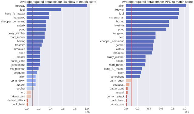
One measure of success is to demonstrate that the model is highly efficient. For this, we evaluated the output of our policies after 100K interactions with the environment, which corresponds to roughly two hours of real-time game play by a person. We compare our SimPLe method with two state of the art model-free RL methods, Rainbow and PPO, applied to 26 different games. In most cases, the SimPLe approach has a sample efficiency more than 2x better than the other methods.
The number of interactions needed by the respective model-free algorithms (left - Rainbow; right - PPO) to match the score achieved using our SimPLe training method. The red line indicates the number of interactions used by our method.
SimPLe Success
An exciting result of the SimPLe approach is that for two of the games, Pong and Freeway, an agent trained in the simulated environment is able to achieve the maximum score. Here is a video of our agent playing the game using the game model that we learned for Pong:
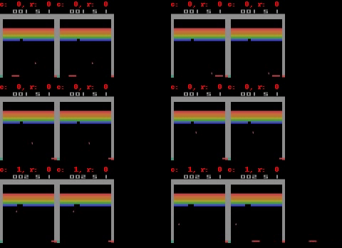
For Freeway, Pong and Breakout, SimPLe can generate nearly pixel-perfect predictions up to 50 steps into the future, as shown below.
Nearly pixel perfect predictions can be made by SimPLe, on Breakout (top) and Freeway (bottom). In each animation, the left is the output of the model, the middle is the groundtruth, and the right pane is the pixel-wise difference between the two.
SimPLe Surprises
SimPLe does not always make correct predictions, however. The most common failure is due to the world model not accurately capturing or predicting small but highly relevant objects. Some examples are: (1) in Atlantis and Battlezone bullets are so small that they tend to disappear, and (2) Private Eye, in which the agent traverses different scenes, teleporting from one to the other. We found that our model generally struggled to capture such large global changes.
In Battlezone, we find the model struggles with predicting small, relevant parts, such as the bullet.
Conclusion
The main promise of model-based reinforcement learning methods is in environments where interactions are either costly, slow or require human labeling, such as many robotics tasks. In such environments, a learned simulator would enable a better understanding of the agent's environment and could lead to new, better and faster ways for doing multi-task reinforcement learning. While SimPLe does not yet match the performance of standard model-free RL methods, it is substantially more efficient, and we expect future work to further improve the performance of model-based techniques.

If you'd like to develop your own models and experiments, head to our repository and colab where you'll find instructions on how to reproduce our work along with pre-trained world models.

Acknowledgements
This work was done in collaboration with the University of Illinois at Urbana-Champaign, the University of Warsaw and deepsense.ai. We would like to give special recognition to paper co-authors Mohammad Babaeizadeh, Piotr Miłos, Błażej Osiński, Roy H Campbell, Konrad Czechowski, Chelsea Finn, Piotr Kozakowski, Sergey Levine, Ryan Sepassi, George Tucker and Henryk Michalewski.

Source: Google AI Blog


Reducing the Need for Labeled Data in Generative Adversarial Networks


Generative adversarial networks (GANs) are a powerful class of deep generative models.The main idea behind GANs is to train two neural networks: the generator, which learns how to synthesise data (such as an image), and the discriminator, which learns how to distinguish real data from the ones synthesised by the generator. This approach has been successfully used for high-fidelity natural image synthesis, improving learned image compression, data augmentation, and more.
Evolution of the generated samples as training progresses on ImageNet. The generator network is conditioned on the class (e.g., "great gray owl" or "golden retriever").
For natural image synthesis, state-of-the-art results are achieved by conditional GANs that, unlike unconditional GANs, use labels (e.g. car, dog, etc.) during training. While this makes the task easier and leads to significant improvements, this approach requires a large amount of labeled data that is rarely available in practice.

In "High-Fidelity Image Generation With Fewer Labels", we propose a new approach to reduce the amount of labeled data required to train state-of-the-art conditional GANs. When combined with recent advancements on large-scale GANs, we match the state-of-the-art in high-fidelity natural image synthesis using 10x fewer labels. Based on this research, we are also releasing a major update to the Compare GAN library, which contains all the components necessary to train and evaluate modern GANs.

Improvements via Semi-supervision and Self-supervision
In conditional GANs, both the generator and discriminator are typically conditioned on class labels. In this work, we propose to replace the hand-annotated ground truth labels with inferred ones. To infer high-quality labels for a large dataset of mostly unlabeled data, we take a two-step approach: First, we learn a feature representation using only the unlabeled portion of the dataset. To learn the feature representations we make use of self-supervision in the form of a recently introduced approach, in which the unlabeled images are randomly rotated and a deep convolutional neural network is tasked with predicting the rotation angle. The idea is that the models need to be able to recognize the main objects and their shapes in order to be successful on this task.
An unlabeled image is randomly rotated and the network is tasked with predicting the rotation angle. Successful models need to capture semantically meaningful image features which can then be used for other vision tasks.
We then consider the activation pattern of one of the intermediate layers of the trained network as the new feature representation of the input, and train a classifier to recognize the label of that input using the labeled portion of the original data set. As the network was pre-trained to extract semantically meaningful features from the data (on the rotation prediction task), training this classifier is more sample-efficient than training the entire network from scratch. Finally, we use this classifier to label the unlabeled data.

To further improve the model quality and training stability we encourage the discriminator network to learn meaningful feature representations which are not forgotten during training by means of an auxiliary loss we introduced previously. These two advancements, combined with large-scale training lead to state-of-the-art conditional GANs for the task of ImageNet synthesis as measured by the Fréchet Inception Distance.
Given a latent vector the generator network produces an image. In each row, linear interpolation between the latent codes of the leftmost and the rightmost image results in a semantic interpolation in the image space.
Compare GAN: A Library for Training and Evaluating GANs
Cutting-edge research on GANs is heavily dependent on a well-engineered and well-tested codebase, since even replicating prior results and techniques requires a significant effort. In order to foster open science and allow the research community benefit from recent advancements, we are releasing a major update of the Compare GAN library. The library includes loss functions, regularization and normalization schemes, neural architectures, and quantitative metrics commonly used in modern GANs, and now supports:
Conclusions and Future Work
Given the growing gap between labeled and unlabeled data sources, it is becoming increasingly important to be able to learn from only partially labeled data. We have shown that a simple yet powerful combination of self-supervision and semi-supervision can help to close this gap for GANs. We believe that self-supervision is a powerful idea that should be investigated for other generative modeling tasks.

Acknowledgments
Work conducted in collaboration with colleagues on the Google Brain team in Zürich, ETH Zürich and UCLA. We would like to thank our paper co-authors Michael Tschannen, Xiaohua Zhai, Olivier Bachem and Sylvain Gelly for their input and feedback. We would like to thank Alexander Kolesnikov, Lucas Beyer and Avital Oliver for helpful discussion on self-supervised learning and semi-supervised learning. We would like to thank Karol Kurach and Marcin Michalski for their major contributions to the Compare GAN library. We would also like to thank Andy Brock, Jeff Donahue and Karen Simonyan for their insights into training GANs on TPUs. The work described in this post also builds upon our work on “Self-Supervised Generative Adversarial Networks” with Ting Chen and Neil Houlsby.

Source: Google AI Blog


Measuring the Limits of Data Parallel Training for Neural Networks


Over the past decade, neural networks have achieved state-of-the-art results in a wide variety of prediction tasks, including image classification, machine translation, and speech recognition. These successes have been driven, at least in part, by hardware and software improvements that have significantly accelerated neural network training. Faster training has directly resulted in dramatic improvements to model quality, both by allowing more training data to be processed and by allowing researchers to try new ideas and configurations more rapidly. Today, hardware developments like Cloud TPU Pods are rapidly increasing the amount of computation available for neural network training, which raises the possibility of harnessing additional computation to make neural networks train even faster and facilitate even greater improvements to model quality. But how exactly should we harness this unprecedented amount of computation, and should we always expect more computation to facilitate faster training?

The most common way to utilize massive compute power is to distribute computations between different processors and perform those computations simultaneously. When training neural networks, the primary ways to achieve this are model parallelism, which involves distributing the neural network across different processors, and data parallelism, which involves distributing training examples across different processors and computing updates to the neural network in parallel. While model parallelism makes it possible to train neural networks that are larger than a single processor can support, it usually requires tailoring the model architecture to the available hardware. In contrast, data parallelism is model agnostic and applicable to any neural network architecture – it is the simplest and most widely used technique for parallelizing neural network training. For the most common neural network training algorithms (synchronous stochastic gradient descent and its variants), the scale of data parallelism corresponds to the batch size, the number of training examples used to compute each update to the neural network. But what are the limits of this type of parallelization, and when should we expect to see large speedups?

In "Measuring the Effects of Data Parallelism in Neural Network Training", we investigate the relationship between batch size and training time by running experiments on six different types of neural networks across seven different datasets using three different optimization algorithms ("optimizers"). In total, we trained over 100K individual models across ~450 workloads, and observed a seemingly universal relationship between batch size and training time across all workloads we tested. We also study how this relationship varies with the dataset, neural network architecture, and optimizer, and found extremely large variation between workloads. Additionally, we are excited to share our raw data for further analysis by the research community. The data includes over 71M model evaluations to make up the training curves of all 100K+ individual models we trained, and can be used to reproduce all 24 plots in our paper.

Universal Relationship Between Batch Size and Training Time
In an idealized data parallel system that spends negligible time synchronizing between processors, training time can be measured in the number of training steps (updates to the neural network's parameters). Under this assumption, we observed three distinct scaling regimes in the relationship between batch size and training time: a "perfect scaling" regime where doubling the batch size halves the number of training steps required to reach a target out-of-sample error, followed by a regime of "diminishing returns", and finally a "maximal data parallelism" regime where further increasing the batch size does not reduce training time, even assuming idealized hardware.

For all workloads we tested, we observed a universal relationship between batch size and training speed with three distinct regimes: perfect scaling (following the dashed line), diminishing returns (diverging from the dashed line), and maximal data parallelism (where the trend plateaus). The transition points between the regimes vary dramatically between different workloads.
Although the basic relationship between batch size and training time appears to be universal, we found that the transition points between the different scaling regimes vary dramatically across neural network architectures and datasets. This means that while simple data parallelism can provide large speedups for some workloads at the limits of today's hardware (e.g. Cloud TPU Pods), and perhaps beyond, some workloads require moving beyond simple data parallelism in order to benefit from the largest scale hardware that exists today, let alone hardware that has yet to be built. For example, in the plot above, ResNet-8 on CIFAR-10 cannot benefit from batch sizes larger than 1,024, whereas ResNet-50 on ImageNet continues to benefit from increasing the batch size up to at least 65,536.

Optimizing Workloads
If one could predict which workloads benefit most from data parallel training, then one could tailor their workloads to make maximal use of the available hardware. However, our results suggest that this will often not be straightforward, because the maximum useful batch size depends, at least somewhat, on every aspect of the workload: the neural network architecture, the dataset, and the optimizer. For example, some neural network architectures can benefit from much larger batch sizes than others, even when trained on the same dataset with the same optimizer. Although this effect sometimes depends on the width and depth of the network, it is inconsistent between different types of network and some networks do not even have obvious notions of "width" and "depth". And while we found that some datasets can benefit from much larger batch sizes than others, these differences are not always explained by the size of the dataset—sometimes smaller datasets benefit more from larger batch sizes than larger datasets.

Left: A transformer neural network scales to much larger batch sizes than an LSTM neural network on the LM1B dataset. Right: The Common Crawl dataset does not benefit from larger batch sizes than the LM1B dataset, even though it is 1,000 times the size.
Perhaps our most promising finding is that even small changes to the optimization algorithm, such as allowing momentum in stochastic gradient descent, can dramatically improve how well training scales with increasing batch size. This raises the possibility of designing new optimizers, or testing the scaling properties of optimizers that we did not consider, to find optimizers that can make maximal use of increased data parallelism.

Future Work
Utilizing additional data parallelism by increasing the batch size is a simple way to produce valuable speedups across a range of workloads, but, for all the workloads we tried, the benefits diminished within the limits of state-of-the-art hardware. However, our results suggest that some optimization algorithms may be able to consistently extend the perfect scaling regime across many models and data sets. Future work could perform the same measurements with other optimizers, beyond the few closely-related ones we tried, to see if any existing optimizer extends perfect scaling across many problems.

Acknowledgements
The authors of this study were Chris Shallue, Jaehoon Lee, Joe Antognini, Jascha Sohl-Dickstein, Roy Frostig and George Dahl (Chris and Jaehoon contributed equally). Many researchers have done work in this area that we have built on, so please see our paper for a full discussion of related work.

Source: Google AI Blog


A Summary of the Google Flood Forecasting Meets Machine Learning Workshop


Recently, we hosted the Google Flood Forecasting Meets Machine Learning workshop in our Tel Aviv office, which brought hydrology and machine learning experts from Google and the broader research community to discuss existing efforts in this space, build a common vocabulary between these groups, and catalyze promising collaborations. In line with our belief that machine learning has the potential to significantly improve flood forecasting efforts and help the hundreds of millions of people affected by floods every year, this workshop discussed improving flood forecasting by aggregating and sharing large data sets, automating calibration and modeling processes, and applying modern statistical and machine learning tools to the problem.

Panel on challenges and opportunities in flood forecasting, featuring (from left to right): Prof. Paolo Burlando (ETH Zürich), Dr. Tyler Erickson (Google Earth Engine), Dr. Peter Salamon (Joint Research Centre) and Prof. Dawei Han (University of Bristol).
The event was kicked off by Google's Yossi Matias, who discussed recent machine learning work and its potential relevance for flood forecasting, crisis response and AI for Social Good, followed by two introductory sessions aimed at bridging some of the knowledge gap between the two fields - introduction to hydrology for computer scientists by Prof. Peter Molnar of ETH Zürich, and introduction to machine learning for hydrologists by Prof. Yishay Mansour of Tel Aviv University and Google

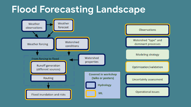
Included in the 2-day event was a wide range of fascinating talks and posters across the flood forecasting landscape, from both hydrologic and machine learning points of view.

An overview of research areas in flood forecasting addressed in the workshop.
Presentations from the research community included:
Alongside these talks, we presented the various efforts across Google to try and improve flood forecasting and foster collaborations in the field, including:
Additionally, at this workshop we piloted an experimental "ML Consultation" panel, where Googlers Gal Elidan, Sasha Goldshtein and Doron Kukliansky gave advice on how to best use machine learning in several hydrology-related tasks. Finally, we concluded the workshop with a moderated panel on the greatest challenges and opportunities in flood forecasting, with hydrology experts Prof. Paolo Burlando of ETH Zürich, Prof. Dawei Han of the University of Bristol, Dr. Peter Salamon of the Joint Research Centre and Dr. Tyler Erickson of Google Earth Engine.
Flood forecasting is an incredibly important and challenging task that is one part of our larger AI for Social Good efforts. We believe that effective global-scale solutions can be achieved by combining modern techniques with the domain expertise already existing in the field. The workshop was a great first step towards creating much-needed understanding, communication and collaboration between the flood forecasting community and the machine learning community, and we look forward to our continued engagement with the broad research community to tackle this challenge.

Acknowledgements
We would like to thank Avinatan Hassidim, Carla Bromberg, Doron Kukliansky, Efrat Morin, Gal Elidan, Guy Shalev, Jennifer Ye, Nadav Rabani and Sasha Goldshtein for their contributions to making this workshop happen.

Source: Google AI Blog


Google Faculty Research Awards 2018


We just completed another round of the Google Faculty Research Awards, our annual open call for proposals on computer science and related topics, such as quantum computing, machine learning, algorithms and theory, natural language processing and more. Our grants cover tuition for a graduate student and provide both faculty and students the opportunity to work directly with Google researchers and engineers.

This round we received 910 proposals covering 40 countries and over 320 universities. After expert reviews and committee discussions, we decided to fund 158 projects. The subject areas that received the most support this year were human computer interaction, machine learning, machine perception, and systems.

Congratulations to the well-deserving recipients of this round's awards. More information on how to apply for the next round will be available at the end of the summer on our website. You can find award recipients from previous years here.

Source: Google AI Blog


Harnessing Organizational Knowledge for Machine Learning


One of the biggest bottlenecks in developing machine learning (ML) applications is the need for the large, labeled datasets used to train modern ML models. Creating these datasets involves the investment of significant time and expense, requiring annotators with the right expertise. Moreover, due to the evolution of real-world applications, labeled datasets often need to be thrown out or re-labeled.

In collaboration with Stanford and Brown University, we present "Snorkel Drybell: A Case Study in Deploying Weak Supervision at Industrial Scale," which explores how existing knowledge in an organization can be used as noisier, higher-level supervision—or, as it is often termed, weak supervision—to quickly label large training datasets. In this study, we use an experimental internal system, Snorkel Drybell, which adapts the open-source Snorkel framework to use diverse organizational knowledge resources—like internal models, ontologies, legacy rules, knowledge graphs and more—in order to generate training data for machine learning models at web scale. We find that this approach can match the efficacy of hand-labeling tens of thousands of data points, and reveals some core lessons about how training datasets for modern machine learning models can be created in practice.

Rather than labeling training data by hand, Snorkel DryBell enables writing labeling functions that label training data programmatically. In this work, we explored how these labeling functions can capture engineers' knowledge about how to use existing resources as heuristics for weak supervision. As an example, suppose our goal is to identify content related to celebrities. One can leverage an existing named-entity recognition (NER) model for this task by labeling any content that does not contain a person as not related to celebrities. This illustrates how existing knowledge resources (in this case, a trained model) can be combined with simple programmatic logic to label training data for a new model. Note also, importantly, that this labeling function returns None---i.e. abstains---in many cases, and thus only labels some small part of the data; our overall goal is to use these labels to train a modern machine learning model that can generalize to new data.

In our example of a labeling function, rather than hand-labeling a data point (1), one utilizes an existing knowledge resource—in this case, a NER model (2)—together with some simple logic expressed in code (3) to heuristically label data.
This programmatic interface for labeling training data is much faster and more flexible than hand-labeling individual data points, but the resulting labels are obviously of much lower quality than manually-specified labels. The labels generated by these labeling functions will often overlap and disagree, as the labeling functions may not only have arbitrary unknown accuracies, but may also be correlated in arbitrary ways (for example, from sharing a common data source or heuristic).

To solve the problem of noisy and correlated labels, Snorkel DryBell uses a generative modeling technique to automatically estimate the accuracies and correlations of the labeling functions in a provably consistent way—without any ground truth training labels—then uses this to re-weight and combine their outputs into a single probabilistic label per data point. At a high level, we rely on the observed agreements and disagreements between the labeling functions (the covariance matrix), and learn the labeling function accuracy and correlation parameters that best explain this observed output using a new matrix completion-style approach. The resulting labels can then be used to train an arbitrary model (e.g. in TensorFlow), as shown in the system diagram below.

Using Diverse Knowledge Sources as Weak Supervision
To study the efficacy of Snorkel Drybell, we used three production tasks and corresponding datasets, aimed at classifying topics in web content, identifying mentions of certain products, and detecting certain real-time events. Using Snorkel DryBell, we were able to make use of various existing or quickly specified sources of information such as:
  • Heuristics and rules: e.g. existing human-authored rules about the target domain.
  • Topic models, taggers, and classifiers: e.g. machine learning models about the target domain or a related domain.
  • Aggregate statistics: e.g. tracked metrics about the target domain.
  • Knowledge or entity graphs: e.g. databases of facts about the target domain.
In Snorkel DryBell, the goal is to train a machine learning model (C), for example to do content or event classification over web data. Rather than hand-labeling training data to do this, in Snorkel DryBell users write labeling functions that express various organizational knowledge resources (A), which are then automatically reweighted and combined (B).
We used these organizational knowledge resources to write labeling functions in a MapReduce template-based pipeline. Each labeling function takes in a data point and either abstains, or outputs a label. The result is a large set of programmatically-generated training labels. However, many of these labels were very noisy (e.g. from the heuristics), conflicted with each other, or were far too coarse-grained (e.g. the topic models) for our task, leading to the next stage of Snorkel DryBell, aimed at automatically cleaning and integrating the labels into a final training set.

Modeling the Accuracies to Combine & Repurpose Existing Sources
To handle these noisy labels, the next stage of Snorkel DryBell combines the outputs from the labeling functions into a single, confidence-weighted training label for each data point. The challenging technical aspect is that this must be done without any ground-truth labels. We use a generative modeling technique that learns the accuracy of each labeling function using only unlabeled data. This technique learns by observing the matrix of agreements and disagreements between the labeling functions' outputs, taking into account known (or statistically estimated) correlation structures between them. In Snorkel DryBell, we also implement a new faster, sampling-free version of this modeling approach, implemented in TensorFlow, in order to handle web-scale data.

By combining and modeling the output of the labeling functions using this procedure in Snorkel DryBell, we were able to generate high-quality training labels. In fact, on the two applications where hand-labeled training data was available for comparison, we achieved the same predictive accuracy training a model with Snorkel DryBell's labels as we did when training that same model with 12,000 and 80,000 hand-labeled training data points.

Transferring Non-Servable Knowledge to Servable Models
In many settings, there is also an important distinction between servable features—which can be used in production—and non-servable features, that are too slow or expensive to be used in production. These non-servable features may have very rich signal, but a general question is how to use them to train or otherwise help servable models that can be deployed in production?


In many settings, users write labeling functions that leverage organizational knowledge resources that are not servable in production (a)—e.g. aggregate statistics, internal models, or knowledge graphs that are too slow or expensive to use in production—in order to train models that are only defined over production-servable features (b), e.g. cheap, real-time web signals.
In Snorkel DryBell, we found that users could write the labeling functions—i.e. express their organizational knowledge—over one feature set that was not servable, and then use the resulting training labels output by Snorkel DryBell to train a model defined over a different, servable feature set. This cross-feature transfer boosted our performance by an average 52% on the benchmark datasets we created. More broadly, it represents a simple but powerful way to use resources that are too slow (e.g. expensive models or aggregate statistics), private (e.g. entity or knowledge graphs), or otherwise unsuitable for deployment, to train servable models over cheap, real-time features. This approach can be viewed as a new type of transfer learning, where instead of transferring a model between different datasets, we're transferring domain knowledge between different feature sets- an approach which has potential use cases not just in industry, but in medical settings and beyond.

Next Steps
Moving forward, we're excited to see what other types of organizational knowledge can be used as weak supervision, and how the approach used by Snorkel DryBell can enable new modes of information reuse and sharing across organizations. For more details, check out our paper, and for further technical details, blog posts, and tutorials, check out the open-source Snorkel implementation at snorkel.stanford.edu.

Acknowledgments
This research was done in collaboration between Google, Stanford, and Brown. We would like to thank all the people who were involved, including Stephen Bach (Brown), Daniel Rodriguez, Yintao Liu, Chong Luo, Haidong Shao, Souvik Sen, Braden Hancock (Stanford), Houman Alborzi, Rahul Kuchhal, Christopher Ré (Stanford), Rob Malkin.

Source: Google AI Blog


An All-Neural On-Device Speech Recognizer


In 2012, speech recognition research showed significant accuracy improvements with deep learning, leading to early adoption in products such as Google's Voice Search. It was the beginning of a revolution in the field: each year, new architectures were developed that further increased quality, from deep neural networks (DNNs) to recurrent neural networks (RNNs), long short-term memory networks (LSTMs), convolutional networks (CNNs), and more. During this time, latency remained a prime focus — an automated assistant feels a lot more helpful when it responds quickly to requests.

Today, we're happy to announce the rollout of an end-to-end, all-neural, on-device speech recognizer to power speech input in Gboard. In our recent paper, "Streaming End-to-End Speech Recognition for Mobile Devices", we present a model trained using RNN transducer (RNN-T) technology that is compact enough to reside on a phone. This means no more network latency or spottiness — the new recognizer is always available, even when you are offline. The model works at the character level, so that as you speak, it outputs words character-by-character, just as if someone was typing out what you say in real-time, and exactly as you'd expect from a keyboard dictation system.
This video compares the production, server-side speech recognizer (left panel) to the new on-device recognizer (right panel) when recognizing the same spoken sentence. Video credit: Akshay Kannan and Elnaz Sarbar
A Bit of History
Traditionally, speech recognition systems consisted of several components - an acoustic model that maps segments of audio (typically 10 millisecond frames) to phonemes, a pronunciation model that connects phonemes together to form words, and a language model that expresses the likelihood of given phrases. In early systems, these components remained independently-optimized.

Around 2014, researchers began to focus on training a single neural network to directly map an input audio waveform to an output sentence. This sequence-to-sequence approach to learning a model by generating a sequence of words or graphemes given a sequence of audio features led to the development of "attention-based" and "listen-attend-spell" models. While these models showed great promise in terms of accuracy, they typically work by reviewing the entire input sequence, and do not allow streaming outputs as the input comes in, a necessary feature for real-time voice transcription.

Meanwhile, an independent technique called connectionist temporal classification (CTC) had helped halve the latency of the production recognizer at that time. This proved to be an important step in creating the RNN-T architecture adopted in this latest release, which can be seen as a generalization of CTC.

Recurrent Neural Network Transducers
RNN-Ts are a form of sequence-to-sequence models that do not employ attention mechanisms. Unlike most sequence-to-sequence models, which typically need to process the entire input sequence (the waveform in our case) to produce an output (the sentence), the RNN-T continuously processes input samples and streams output symbols, a property that is welcome for speech dictation. In our implementation, the output symbols are the characters of the alphabet. The RNN-T recognizer outputs characters one-by-one, as you speak, with white spaces where appropriate. It does this with a feedback loop that feeds symbols predicted by the model back into it to predict the next symbols, as described in the figure below.
Representation of an RNN-T, with the input audio samples, x, and the predicted symbols y. The predicted symbols (outputs of the Softmax layer) are fed back into the model through the Prediction network, as yu-1, ensuring that the predictions are conditioned both on the audio samples so far and on past outputs. The Prediction and Encoder Networks are LSTM RNNs, the Joint model is a feedforward network (paper). The Prediction Network comprises 2 layers of 2048 units, with a 640-dimensional projection layer. The Encoder Network comprises 8 such layers. Image credit: Chris Thornton
Training such models efficiently was already difficult, but with our development of a new training technique that further reduced the word error rate by 5%, it became even more computationally intensive. To deal with this, we developed a parallel implementation so the RNN-T loss function could run efficiently in large batches on Google's high-performance Cloud TPU v2 hardware. This yielded an approximate 3x speedup in training.

Offline Recognition
In a traditional speech recognition engine, the acoustic, pronunciation, and language models we described above are "composed" together into a large search graph whose edges are labeled with the speech units and their probabilities. When a speech waveform is presented to the recognizer, a "decoder" searches this graph for the path of highest likelihood, given the input signal, and reads out the word sequence that path takes. Typically, the decoder assumes a Finite State Transducer (FST) representation of the underlying models. Yet, despite sophisticated decoding techniques, the search graph remains quite large, almost 2GB for our production models. Since this is not something that could be hosted easily on a mobile phone, this method requires online connectivity to work properly.

To improve the usefulness of speech recognition, we sought to avoid the latency and inherent unreliability of communication networks by hosting the new models directly on device. As such, our end-to-end approach does not need a search over a large decoder graph. Instead, decoding consists of a beam search through a single neural network. The RNN-T we trained offers the same accuracy as the traditional server-based models but is only 450MB, essentially making a smarter use of parameters and packing information more densely. However, even on today's smartphones, 450MB is a lot, and propagating signals through such a large network can be slow.

We further reduced the model size by using the parameter quantization and hybrid kernel techniques we developed in 2016 and made publicly available through the model optimization toolkit in the TensorFlow Lite library. Model quantization delivered a 4x compression with respect to the trained floating point models and a 4x speedup at run-time, enabling our RNN-T to run faster than real time speech on a single core. After compression, the final model is 80MB.

Our new all-neural, on-device Gboard speech recognizer is initially being launched to all Pixel phones in American English only. Given the trends in the industry, with the convergence of specialized hardware and algorithmic improvements, we are hopeful that the techniques presented here can soon be adopted in more languages and across broader domains of application.

Acknowledgements:
Raziel Alvarez, Michiel Bacchiani, Tom Bagby, Françoise Beaufays, Deepti Bhatia, Shuo-yiin Chang, Yanzhang He, Alex Gruenstein, Anjuli Kannan, Bo Li, Qiao Liang, Ian McGraw, Ruoming Pang, Rohit Prabhavalkar, Golan Pundak, Kanishka Rao, David Rybach, Tara Sainath, Haşim Sak, June Yuan Shangguan, Matt Shannon, Mohammadinamul Sheik, Khe Chai Sim, Gabor Simko, Trevor Strohman, Mirkó Visontai, Yonghui Wu, Ding Zhao, Dan Zivkovic.

Source: Google AI Blog


Real-Time AR Self-Expression with Machine Learning


Augmented reality (AR) helps you do more with what you see by overlaying digital content and information on top of the physical world. For example, AR features coming to Google Maps will let you find your way with directions overlaid on top of your real world. With Playground - a creative mode in the Pixel camera -- you can use AR to see the world differently. And with the latest release of YouTube Stories and ARCore's new Augmented Faces API you can add objects like animated masks, glasses, 3D hats and more to your own selfies!

One of the key challenges in making these AR features possible is proper anchoring of the virtual content to the real world; a process that requires a unique set of perceptive technologies able to track the highly dynamic surface geometry across every smile, frown or smirk.
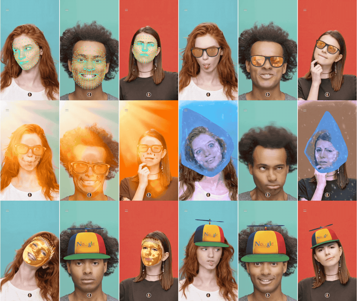
Our 3D mesh and some of the effects it enables
To make all this possible, we employ machine learning (ML) to infer approximate 3D surface geometry to enable visual effects, requiring only a single camera input without the need for a dedicated depth sensor. This approach provides the use of AR effects at realtime speeds, using TensorFlow Lite for mobile CPU inference or its new mobile GPU functionality where available. This technology is the same as what powers YouTube Stories' new creator effects, and is also available to the broader developer community via the latest ARCore SDK release and the ML Kit Face Contour Detection API.

An ML Pipeline for Selfie AR
Our ML pipeline consists of two real-time deep neural network models that work together: A detector that operates on the full image and computes face locations, and a generic 3D mesh model that operates on those locations and predicts the approximate surface geometry via regression. Having the face accurately cropped drastically reduces the need for common data augmentations like affine transformations consisting of rotations, translation and scale changes. Instead it allows the network to dedicate most of its capacity towards coordinate prediction accuracy, which is critical to achieve proper anchoring of the virtual content.

Once the location of interest is cropped, the mesh network is only applied to a single frame at a time, using a windowed smoothing in order to reduce noise when the face is static while avoiding lagging during significant movement.
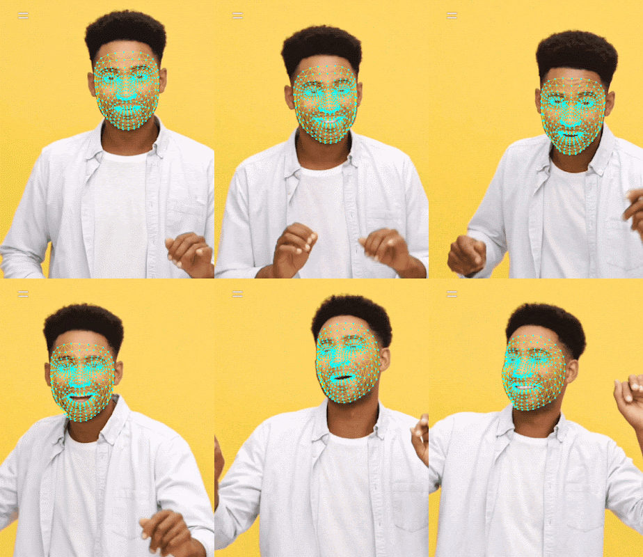
Our 3D mesh in action
For our 3D mesh we employed transfer learning and trained a network with several objectives: the network simultaneously predicts 3D mesh coordinates on synthetic, rendered data and 2D semantic contours on annotated, real world data similar to those MLKit provides. The resulting network provided us with reasonable 3D mesh predictions not just on synthetic but also on real world data. All models are trained on data sourced from a geographically diverse dataset and subsequently tested on a balanced, diverse testset for qualitative and quantitative performance.

The 3D mesh network receives as input a cropped video frame. It doesn't rely on additional depth input, so it can also be applied to pre-recorded videos. The model outputs the positions of the 3D points, as well as the probability of a face being present and reasonably aligned in the input. A common alternative approach is to predict a 2D heatmap for each landmark, but it is not amenable to depth prediction and has high computational costs for so many points.

We further improve the accuracy and robustness of our model by iteratively bootstrapping and refining predictions. That way we can grow our dataset to increasingly challenging cases, such as grimaces, oblique angle and occlusions. Dataset augmentation techniques also expanded the available ground truth data, developing model resilience to artifacts like camera imperfections or extreme lighting conditions.
Dataset expansion and improvement pipeline
Hardware-tailored Inference
We use TensorFlow Lite for on-device neural network inference. The newly introduced GPU back-end acceleration boosts performance where available, and significantly lowers the power consumption. Furthermore, to cover a wide range of consumer hardware, we designed a variety of model architectures with different performance and efficiency characteristics. The most important differences of the lighter networks are the residual block layout and the accepted input resolution (128x128 pixels in the lightest model vs. 256x256 in the most complex). We also vary the number of layers and the subsampling rate (how fast the input resolution decreases with network depth).
Inference time per frame: CPU vs. GPU
The result of these optimizations is a substantial speedup from using lighter models, with minimal degradation in AR effect quality.
Comparison of the most complex (left) and the lightest models (right). Temporal consistency as well as lip and eye tracking is slightly degraded on light models.
The end result of these efforts empowers a user experience with convincing, realistic selfie AR effects in YouTube, ARCore, and other clients by:
  • Simulating light reflections via environmental mapping for realistic rendering of glasses
  • Natural lighting by casting virtual object shadows onto the face mesh
  • Modelling face occlusions to hide virtual object parts behind a face, e.g. virtual glasses, as shown below.
YouTube Stories includes Creator Effects like realistic virtual glasses, based on our 3D mesh
In addition, we achieve highly realistic makeup effects by:
  • Modelling Specular reflections applied on lips and
  • Face painting by using luminance-aware material 
Case study comparing real make-up against our AR make-up on 5 subjects under different lighting conditions.
We are excited to share this new technology with creators, users and developers alike, who can use this new technology immediately by downloading the latest ARCore SDK. In the future we plan to broaden this technology to more Google products.

Acknowledgements
We would like to thank Yury Kartynnik, Valentin Bazarevsky, Andrey Vakunov, Siargey Pisarchyk, Andrei Tkachenka, and Matthias Grundmann for collaboration on developing the current mesh technology; Nick Dufour, Avneesh Sud and Chris Bregler for an earlier version of the technology based on parametric models; Kanstantsin Sokal, Matsvei Zhdanovich, Gregory Karpiak, Alexander Kanaukou, Suril Shah, Buck Bourdon, Camillo Lugaresi, Siarhei Kazakou and Igor Kibalchich for building the ML pipeline to drive impressive effects; Aleksandra Volf and the annotation team for their diligence and dedication to perfection; Andrei Kulik, Juhyun Lee, Raman Sarokin, Ekaterina Ignasheva, Nikolay Chirkov, and Yury Pisarchyk for careful benchmarking and insights on mobile GPU-centric network architecture optimizations.

Source: Google AI Blog