Tag Archives: machine learning

Introduction to Fairness in Machine Learning

Posted by Andrew Zaldivar, Developer Advocate, Google AI

A few months ago, we announced our AI Principles, a set of commitments we are upholding to guide our work in artificial intelligence (AI) going forward. Along with our AI Principles, we shared a set of recommended practices to help the larger community design and build responsible AI systems.

In particular, one of our AI Principles speaks to the importance of recognizing that AI algorithms and datasets are the product of the environment—and, as such, we need to be conscious of any potential unfair outcomes generated by an AI system and the risk it poses across cultures and societies. A recommended practice here for practitioners is to understand the limitations of their algorithm and datasets—but this is a problem that is far from solved.

To help practitioners take on the challenge of building fairer and more inclusive AI systems, we developed a short, self-study training module on fairness in machine learning. This new module is part of our Machine Learning Crash Course, which we highly recommend taking first—unless you know machine learning really well, in which case you can jump right into the Fairness module.

The Fairness module features a hands-on technical exercise. This exercise demonstrates how you can use tools and techniques that may already exist in your development stack (such as Facets Dive, Seaborn, pandas, scikit-learn and TensorFlow Estimators to name a few) to explore and discover ways to make your machine learning system fairer and more inclusive. We created our exercise in a Colaboratory notebook, which you are more than welcome to use, modify and distribute for your own purposes.

From exploring datasets to analyzing model performance, it's really easy to forget to make time for responsible reflection when building an AI system. So rather than having you run every code cell in sequential order without pause, we added what we call FairAware tasks throughout the exercise. FairAware tasks help you zoom in and out of the problem space. That way, you can remind yourself of the big picture: finding the undesirable biases that could disproportionately affect model performance across groups. We hope a process like FairAware will become part of your workflow, helping you find opportunities for inclusion.

FairAware task guiding practitioner to compare performances across gender.

The Fairness module was created to provide you with enough of an understanding to get started in addressing fairness and inclusion in AI. Keep an eye on this space for future work as this is only the beginning.

If you wish to learn more from our other examples, check out the Fairness section of our Responsible AI Practices guide. There, you will find a full set of Google recommendations and resources. From our latest research proposal on reporting model performance with fairness and inclusion considerations, to our recently launched diagnostic tool that lets anyone investigate trained models for fairness, our resource guide highlights many areas of research and development in fairness.

Let us know what your thoughts are on our Fairness module. If you have any specific comments on the notebook exercise itself, then feel free to leave a comment on our GitHub repo.


On behalf of many contributors and supporters,

Andrew Zaldivar – Developer Advocate, Google AI

Combating Potentially Harmful Applications with Machine Learning at Google: Datasets and Models

Posted by Mo Yu, Android Security & Privacy Team

In a previous blog post, we talked about using machine learning to combat Potentially Harmful Applications (PHAs). This blog post covers how Google uses machine learning techniques to detect and classify PHAs. We'll discuss the challenges in the PHA detection space, including the scale of data, the correct identification of PHA behaviors, and the evolution of PHA families. Next, we will introduce two of the datasets that make the training and implementation of machine learning models possible, such as app analysis data and Google Play data. Finally, we will present some of the approaches we use, including logistic regression and deep neural networks.

Using machine learning to scale

Detecting PHAs is challenging and requires a lot of resources. Our security experts need to understand how apps interact with the system and the user, analyze complex signals to find PHA behavior, and evolve their tactics to stay ahead of PHA authors. Every day, Google Play Protect (GPP) analyzes over half a million apps, which makes a lot of new data for our security experts to process.

Leveraging machine learning helps us detect PHAs faster and at a larger scale. We can detect more PHAs just by adding additional computing resources. In many cases, machine learning can find PHA signals in the training data without human intervention. Sometimes, those signals are different than signals found by security experts. Machine learning can take better advantage of this data, and discover hidden relationships between signals more effectively.

There are two major parts of Google Play Protect's machine learning protections: the data and the machine learning models.

Data sources

The quality and quantity of the data used to create a model are crucial to the success of the system. For the purpose of PHA detection and classification, our system mainly uses two anonymous data sources: data from analyzing apps and data from how users experience apps.

App data

Google Play Protect analyzes every app that it can find on the internet. We created a dataset by decomposing each app's APK and extracting PHA signals with deep analysis. We execute various processes on each app to find particular features and behaviors that are relevant to the PHA categories in scope (for example, SMS fraud, phishing, privilege escalation). Static analysis examines the different resources inside an APK file while dynamic analysis checks the behavior of the app when it's actually running. These two approaches complement each other. For example, dynamic analysis requires the execution of the app regardless of how obfuscated its code is (obfuscation hinders static analysis), and static analysis can help detect cloaking attempts in the code that may in practice bypass dynamic analysis-based detection. In the end, this analysis produces information about the app's characteristics, which serve as a fundamental data source for machine learning algorithms.

Google Play data

In addition to analyzing each app, we also try to understand how users perceive that app. User feedback (such as the number of installs, uninstalls, user ratings, and comments) collected from Google Play can help us identify problematic apps. Similarly, information about the developer (such as the certificates they use and their history of published apps) contribute valuable knowledge that can be used to identify PHAs. All these metrics are generated when developers submit a new app (or new version of an app) and by millions of Google Play users every day. This information helps us to understand the quality, behavior, and purpose of an app so that we can identify new PHA behaviors or identify similar apps.

In general, our data sources yield raw signals, which then need to be transformed into machine learning features for use by our algorithms. Some signals, such as the permissions that an app requests, have a clear semantic meaning and can be directly used. In other cases, we need to engineer our data to make new, more powerful features. For example, we can aggregate the ratings of all apps that a particular developer owns, so we can calculate a rating per developer and use it to validate future apps. We also employ several techniques to focus in on interesting data.To create compact representations for sparse data, we use embedding. To help streamline the data to make it more useful to models, we use feature selection. Depending on the target, feature selection helps us keep the most relevant signals and remove irrelevant ones.

By combining our different datasets and investing in feature engineering and feature selection, we improve the quality of the data that can be fed to various types of machine learning models.

Models

Building a good machine learning model is like building a skyscraper: quality materials are important, but a great design is also essential. Like the materials in a skyscraper, good datasets and features are important to machine learning, but a great algorithm is essential to identify PHA behaviors effectively and efficiently.

We train models to identify PHAs that belong to a specific category, such as SMS-fraud or phishing. Such categories are quite broad and contain a large number of samples given the number of PHA families that fit the definition. Alternatively, we also have models focusing on a much smaller scale, such as a family, which is composed of a group of apps that are part of the same PHA campaign and that share similar source code and behaviors. On the one hand, having a single model to tackle an entire PHA category may be attractive in terms of simplicity but precision may be an issue as the model will have to generalize the behaviors of a large number of PHAs believed to have something in common. On the other hand, developing multiple PHA models may require additional engineering efforts, but may result in better precision at the cost of reduced scope.

We use a variety of modeling techniques to modify our machine learning approach, including supervised and unsupervised ones.

One supervised technique we use is logistic regression, which has been widely adopted in the industry. These models have a simple structure and can be trained quickly. Logistic regression models can be analyzed to understand the importance of the different PHA and app features they are built with, allowing us to improve our feature engineering process. After a few cycles of training, evaluation, and improvement, we can launch the best models in production and monitor their performance.

For more complex cases, we employ deep learning. Compared to logistic regression, deep learning is good at capturing complicated interactions between different features and extracting hidden patterns. The millions of apps in Google Play provide a rich dataset, which is advantageous to deep learning.

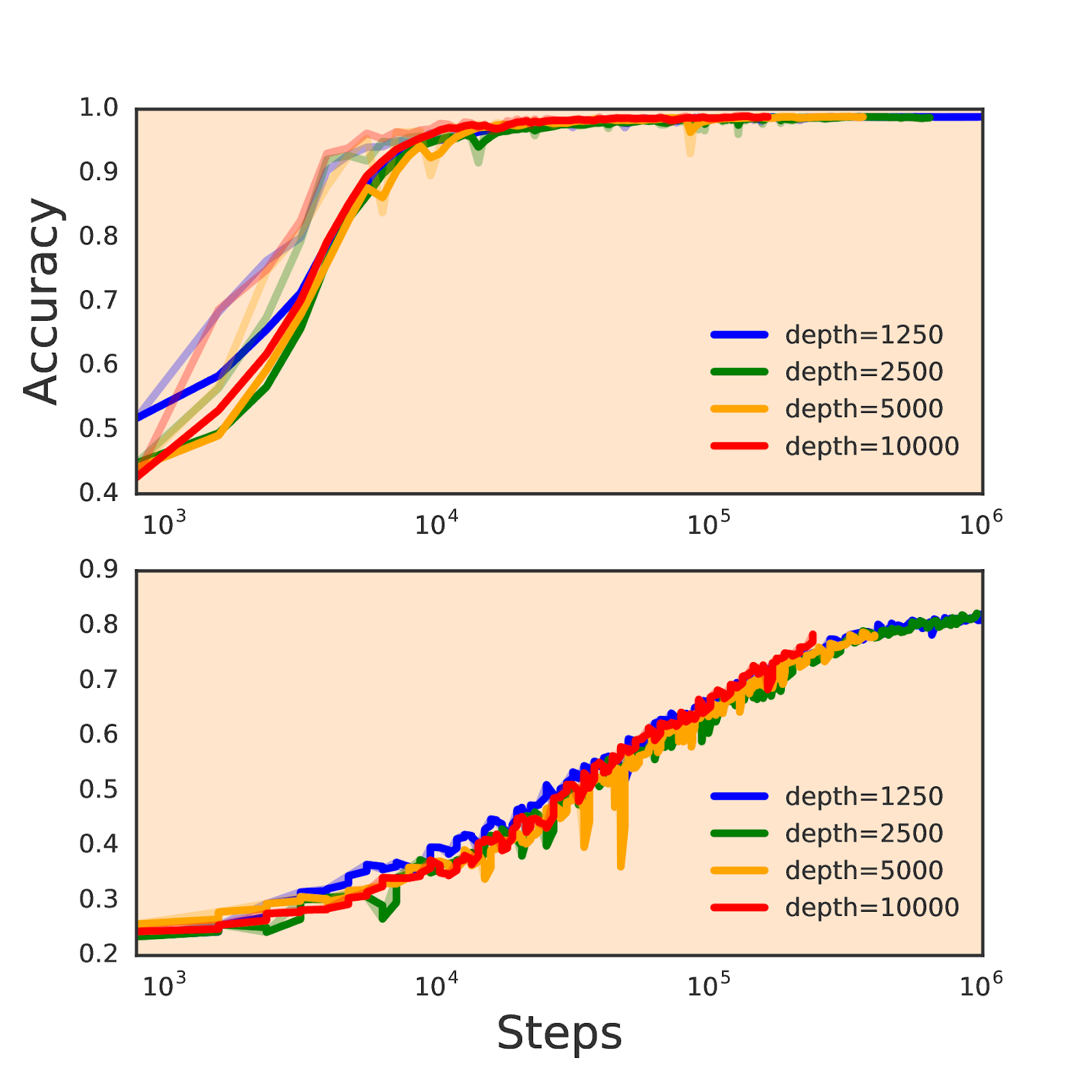
In addition to our targeted feature engineering efforts, we experiment with many aspects of deep neural networks. For example, a deep neural network can have multiple layers and each layer has several neurons to process signals. We can experiment with the number of layers and neurons per layer to change model behaviors.

We also adopt unsupervised machine learning methods. Many PHAs use similar abuse techniques and tricks, so they look almost identical to each other. An unsupervised approach helps define clusters of apps that look or behave similarly, which allows us to mitigate and identify PHAs more effectively. We can automate the process of categorizing that type of app if we are confident in the model or can request help from a human expert to validate what the model found.

PHAs are constantly evolving, so our models need constant updating and monitoring. In production, models are fed with data from recent apps, which help them stay relevant. However, new abuse techniques and behaviors need to be continuously detected and fed into our machine learning models to be able to catch new PHAs and stay on top of recent trends. This is a continuous cycle of model creation and updating that also requires tuning to ensure that the precision and coverage of the system as a whole matches our detection goals.

Looking forward

As part of Google's AI-first strategy, our work leverages many machine learning resources across the company, such as tools and infrastructures developed by Google Brain and Google Research. In 2017, our machine learning models successfully detected 60.3% of PHAs identified by Google Play Protect, covering over 2 billion Android devices. We continue to research and invest in machine learning to scale and simplify the detection of PHAs in the Android ecosystem.

Acknowledgements

This work was developed in joint collaboration with Google Play Protect, Safe Browsing and Play Abuse teams with contributions from Andrew Ahn, Hrishikesh Aradhye, Daniel Bali, Hongji Bao, Yajie Hu, Arthur Kaiser, Elena Kovakina, Salvador Mandujano, Melinda Miller, Rahul Mishra, Damien Octeau, Sebastian Porst, Chuangang Ren, Monirul Sharif, Sri Somanchi, Sai Deep Tetali, Zhikun Wang, and Mo Yu.

Introducing AdaNet: Fast and Flexible AutoML with Learning Guarantees


Ensemble learning, the art of combining different machine learning (ML) model predictions, is widely used with neural networks to achieve state-of-the-art performance, benefitting from a rich history and theoretical guarantees to enable success at challenges such as the Netflix Prize and various Kaggle competitions. However, they aren’t used much in practice due to long training times, and the ML model candidate selection requires its own domain expertise. But as computational power and specialized deep learning hardware such as TPUs become more readily available, machine learning models will grow larger and ensembles will become more prominent. Now, imagine a tool that automatically searches over neural architectures, and learns to combine the best ones into a high-quality model.

Today, we’re excited to share AdaNet, a lightweight TensorFlow-based framework for automatically learning high-quality models with minimal expert intervention. AdaNet builds on our recent reinforcement learning and evolutionary-based AutoML efforts to be fast and flexible while providing learning guarantees. Importantly, AdaNet provides a general framework for not only learning a neural network architecture, but also for learning to ensemble to obtain even better models.

AdaNet is easy to use, and creates high-quality models, saving ML practitioners the time normally spent selecting optimal neural network architectures, implementing an adaptive algorithm for learning a neural architecture as an ensemble of subnetworks. AdaNet is capable of adding subnetworks of different depths and widths to create a diverse ensemble, and trade off performance improvement with the number of parameters.
AdaNet adaptively growing an ensemble of neural networks. At each iteration, it measures the ensemble loss for each candidate, and selects the best one to move onto the next iteration.
Fast and Easy to Use
AdaNet implements the TensorFlow Estimator interface, which greatly simplifies machine learning programming by encapsulating training, evaluation, prediction and export for serving. It integrates with open-source tools like TensorFlow Hub modules, TensorFlow Model Analysis, and Google Cloud’s Hyperparameter Tuner. Distributed training support significantly reduces training time, and scales linearly with available CPUs and accelerators (e.g. GPUs).
AdaNet’s accuracy (y-axis) per train step (x-axis) on CIFAR-100. The blue line is accuracy on the training set, and red line is performance on the test set. A new subnetwork begins training every million steps, and eventually improves the performance of the ensemble. The grey and green lines are the accuracies of the ensemble before adding the new subnetwork.
Because TensorBoard is one of the best TensorFlow features for visualizing model metrics during training, AdaNet integrates seamlessly with it in order to monitor subnetwork training, ensemble composition, and performance. When AdaNet is done training, it exports a SavedModel that can be deployed with TensorFlow Serving.

Learning Guarantees
Building an ensemble of neural networks has several challenges: What are the best subnetwork architectures to consider? Is it best to reuse the same architectures or encourage diversity? While complex subnetworks with more parameters will tend to perform better on the training set, they may not generalize to unseen data due to their greater complexity. These challenges stem from evaluating model performance. We could evaluate performance on a hold-out set split from the training set, but in doing so would reduce the number of examples one can use for training the neural network.

Instead, AdaNet’s approach (presented in “AdaNet: Adaptive Structural Learning of Artificial Neural Networks” at ICML 2017) is to optimize an objective that balances the trade-offs between the ensemble’s performance on the training set and its ability to generalize to unseen data. The intuition is for the ensemble to include a candidate subnetwork only when it improves the ensemble’s training loss more than it affects its ability to generalize. This guarantees that:
  1. The generalization error of the ensemble is bounded by its training error and complexity.
  2. By optimizing this objective, we are directly minimizing this bound.
A practical benefit of optimizing this objective is that it eliminates the need for a hold-out set for choosing which candidate subnetworks to add to the ensemble. This has the added benefit of enabling the use of more training data for training the subnetworks. To learn more, please walk through our tutorial about the AdaNet objective.

Extensible
We believe that the key to making a useful AutoML framework for both research and production use is to not only provide sensible defaults, but to also allow users to try their own subnetwork/model definitions. As a result, machine learning researchers, practitioners, and enthusiasts are invited to define their own AdaNet adanet.subnetwork.Builder using high level TensorFlow APIs like tf.layers.

Users who have already integrated a TensorFlow model in their system can easily convert their TensorFlow code into an AdaNet subnetwork, and use the adanet.Estimator to boost model performance while obtaining learning guarantees. AdaNet will explore their defined search space of candidate subnetworks and learn to ensemble the subnetworks. For instance, we took an open-source implementation of a NASNet-A CIFAR architecture, transformed it into a subnetwork, and improved upon CIFAR-10 state-of-the-art results after eight AdaNet iterations. Furthermore, our model achieves this result with fewer parameters:
Performance of a NASNet-A model as presented in Zoph et al., 2018 versus AdaNet learning to combine small NASNet-A subnetworks on CIFAR-10.
Users are also invited to use their own custom loss functions as part of the AdaNet objective via canned or custom tf.contrib.estimator.Heads in order to train regression, classification, and multi-task learning problems.

Users can also fully define the search space of candidate subnetworks to explore by extending the adanet.subnetwork.Generator class. This allows them to grow or reduce their search space based on their available hardware. The search space of subnetworks can be as simple as duplicating the same subnetwork configuration with different random seeds, to training dozens of subnetworks with different hyperparameter combinations, and letting AdaNet choose the one to include in the final ensemble.

If you’re interested in trying AdaNet for yourself, please check out our Github repo, and walk through the tutorial notebooks. We’ve included a few working examples using dense layers and convolutions to get you started. AdaNet is an ongoing research project, and we welcome contributions. We’re excited to see how AdaNet can help the research community.

Acknowledgements
This project was only possible thanks to the members of the core team including Corinna Cortes, Mehryar Mohri, Xavi Gonzalvo, Charles Weill, Vitaly Kuznetsov, Scott Yak, and Hanna Mazzawi. We also extend a special thanks to our collaborators, residents and interns Gus Kristiansen, Galen Chuang, Ghassen Jerfel, Vladimir Macko, Ben Adlam, Scott Yang and the many others at Google who helped us test it out.

Source: Google AI Blog


Curiosity and Procrastination in Reinforcement Learning


Reinforcement learning (RL) is one of the most actively pursued research techniques of machine learning, in which an artificial agent receives a positive reward when it does something right, and negative reward otherwise. This carrot-and-stick approach is simple and universal, and allowed DeepMind to teach the DQN algorithm to play vintage Atari games and AlphaGoZero to play the ancient game of Go. This is also how OpenAI taught its OpenAI-Five algorithm to play the modern video game Dota, and how Google taught robotic arms to grasp new objects. However, despite the successes of RL, there are many challenges to making it an effective technique.

Standard RL algorithms struggle with environments where feedback to the agent is sparse — crucially, such environments are common in the real world. As an example, imagine trying to learn how to find your favorite cheese in a large maze-like supermarket. You search and search but the cheese section is nowhere to be found. If at every step you receive no “carrot” and no “stick”, there’s no way to tell if you are headed in the right direction or not. In the absence of rewards, what is to stop you from wandering around in circles? Nothing, except perhaps your curiosity, which motivates you go into a product section that looks unfamiliar to you in pursuit of your sought-after cheese.

In “Episodic Curiosity through Reachability” — the result of a collaboration between the Google Brain team, DeepMind and ETH Zürich — we propose a novel episodic memory-based model of granting RL rewards, akin to curiosity, which leads to exploring the environment. Since we want the agent not only to explore the environment but also to solve the original task, we add a reward bonus provided by our model to the original sparse task reward. The combined reward is not sparse anymore which allows standard RL algorithms to learn from it. Thus, our curiosity method expands the set of tasks which are solvable with RL.
Episodic Curiosity through Reachability: Observations are added to memory, reward is computed based on how far the current observation is from the most similar observation in memory. The agent receives more reward for seeing observations which are not yet represented in memory.
The key idea of our method is to store the agent's observations of the environment in an episodic memory, while also rewarding the agent for reaching observations not yet represented in memory. Being “not in memory” is the definition of novelty in our method — seeking such observations means seeking the unfamiliar. Such a drive to seek the unfamiliar will lead the artificial agent to new locations, thus keeping it from wandering in circles and ultimately help it stumble on the goal. As we will discuss later, our formulation can save the agent from undesired behaviours which some other formulations are prone to. Much to our surprise, those behaviours bear some similarity to what a layperson would call “procrastination”.

Previous Curiosity Formulations
While there have been many attempts to formulate curiosity in the past[1][2][3][4], in this post we  focus on one natural and very popular approach: curiosity through prediction-based surprise, explored in the recent paper “Curiosity-driven Exploration by Self-supervised Prediction” (commonly referred to as the ICM method). To illustrate how surprise leads to curiosity, again consider our analogy of looking for cheese in a supermarket.
Illustration © Indira Pasko, used under CC BY-NC-ND 4.0 license.
As you wander throughout the market, you try to predict the future (“Now I’m in the meat section, so I think the section around the corner is the fish section — those are usually adjacent in this supermarket chain”). If your prediction is wrong, you are surprised (“No, it’s actually the vegetables section. I didn’t expect that!”) and thus rewarded. This makes you more motivated to look around the corner in the future, exploring new locations just to see if your expectations about them meet the reality (and, hopefully, stumble upon the cheese).

Similarly, the ICM method builds a predictive model of the dynamics of the world and gives the agent rewards when the model fails to make good predictions — a marker of surprise or novelty. Note that exploring unvisited locations is not directly a part of the ICM curiosity formulation. For the ICM method, visiting them is only a way to obtain more “surprise” and thus maximize overall rewards. As it turns out, in some environments there could be other ways to inflict self-surprise, leading to unforeseen results.
Agent imbued with surprise-based curiosity gets stuck when it encounters TV. GIF adopted from a video by © Deepak Pathak, used under CC BY 2.0 license.
The Dangers of “Procrastination”
In "Large-Scale Study of Curiosity-Driven Learning", the authors of the ICM method along with researchers from OpenAI show a hidden danger of surprise maximization: agents can learn to indulge procrastination-like behaviour instead of doing something useful for the task at hand. To see why, consider a common thought experiment the authors call the “noisy TV problem”, in which an agent is put into a maze and tasked with finding a highly rewarding item (akin to “cheese” in our previous supermarket example). The environment also contains a TV for which the agent has the remote control. There is a limited number of channels (each with a distinct show) and every press on the remote control switches to a random channel. How would an agent perform in such an environment?

For the surprise-based curiosity formulation, changing channels would result in a large reward, as each change is unpredictable and surprising. Crucially, even after cycling through all the available channels, the random channel selection ensures every new change will still be surprising — the agent is making predictions about what will be on the TV after a channel change, and will very likely be wrong, leading to surprise. Importantly, even if the agent has already seen every show on every channel, the change is still unpredictable. Because of this, the agent imbued with surprise-based curiosity would eventually stay in front of the TV forever instead of searching for a highly rewarding item — akin to procrastination. So, what would be a definition of curiosity which does not lead to such behaviour?

Episodic Curiosity
In “Episodic Curiosity through Reachability”, we explore an episodic memory-based curiosity model that turns out to be less prone to “self-indulging” instant gratification. Why so? Using our example above, after changing channels for a while, all of the shows will end up in memory. Thus, the TV won’t be so attractive anymore: even if the order of shows appearing on the screen is random and unpredictable, all those shows are already in memory! This is the main difference to the surprise-based methods: our method doesn’t even try to make bets about the future which could be hard (or even impossible) to predict. Instead, the agent examines the past to know if it has seen observations similar to the current one. Thus our agent won’t be drawn that much to the instant gratification provided by the noisy TV. It will have to go and explore the world outside of the TV to get more reward.

But how do we decide whether the agent is seeing the same thing as an existing memory? Checking for an exact match could be meaningless: in a realistic environment, the agent rarely sees exactly the same thing twice. For example, even if the agent returned to exactly the same room, it would still see this room under a different angle compared to its memories.

Instead of checking for an exact match in memory, we use a deep neural network that is trained to measure how similar two experiences are. To train this network, we have it guess whether two observations were experienced close together in time, or far apart in time. Temporal proximity is a good proxy for whether two experiences should be judged to be part of the same experience. This training leads to a general concept of novelty via reachability which is illustrated below.
Graph of reachabilities would determine novelty. In practice, this graph is not available — so we train a neural network approximator to estimate a number of steps between observations.
Experimental Results
To compare the performance of different approaches to curiosity, we tested them in two visually rich 3D environments: ViZDoom and DMLab. In those environments, the agent was tasked with various problems like searching for a goal in a maze or collecting good and avoiding bad objects. The DMLab environment happens to provide the agent with a laser-like science fiction gadget. The standard setting in the previous work on DMLab was to equip the agent with this gadget for all tasks, and if the agent does not need a gadget for a particular task, it is free not to use it. Interestingly, similar to the noisy TV experiment described above, the surprise-based ICM method actually uses this gadget a lot even when it is useless for the task at hand! When tasked with searching for a high-rewarding item in the maze, it instead prefers to spend time tagging walls because this yields a lot of “surprise” reward. Theoretically, predicting the result of tagging should be possible, but in practice is too hard as it apparently requires a deeper knowledge of physics than is available to a standard agent.
Surprise-based ICM method is persistently tagging the wall instead of exploring the maze.
Our method instead learns reasonable exploration behaviour under the same conditions. This is because it does not try to predict the result of its actions, but rather seeks observations which are “harder” to achieve from those already in the episodic memory. In other words, the agent implicitly pursues goals which require more effort to reach from memory than just a single tagging action.
Our method shows reasonable exploration.
It is interesting to see that our approach to granting reward penalizes an agent running in circles. This is because after completing the first circle the agent does not encounter new observations other than those in memory, and thus receives no reward:
Our reward visualization: red means negative reward, green means positive reward. Left to right: map with rewards, map with locations currently in memory, first-person view.
At the same time, our method favors good exploration behavior:
Our reward visualization: red means negative reward, green means positive reward. Left to right: map with rewards, map with locations currently in memory, first-person view.
We hope that our work will help lead to a new wave of exploration methods, going beyond surprise and learning more intelligent exploration behaviours. For an in-depth analysis of our method, please take a look at the preprint of our research paper.

Acknowledgements:
This project is a result of a collaboration between the Google Brain team, DeepMind and ETH Zürich. The core team includes Nikolay Savinov, Anton Raichuk, Raphaël Marinier, Damien Vincent, Marc Pollefeys, Timothy Lillicrap and Sylvain Gelly. We would like to thank Olivier Pietquin, Carlos Riquelme, Charles Blundell and Sergey Levine for the discussions about the paper. We are grateful to Indira Pasko for the help with illustrations.

References:
[1] "Count-Based Exploration with Neural Density Models", Georg Ostrovski, Marc G. Bellemare, Aaron van den Oord, Remi Munos
[2] "#Exploration: A Study of Count-Based Exploration for Deep Reinforcement Learning", Haoran Tang, Rein Houthooft, Davis Foote, Adam Stooke, Xi Chen, Yan Duan, John Schulman, Filip De Turck, Pieter Abbeel
[3] "Unsupervised Learning of Goal Spaces for Intrinsically Motivated Goal Exploration", Alexandre Péré, Sébastien Forestier, Olivier Sigaud, Pierre-Yves Oudeyer
[4] "VIME: Variational Information Maximizing Exploration", Rein Houthooft, Xi Chen, Yan Duan, John Schulman, Filip De Turck, Pieter Abbeel

Source: Google AI Blog


Fluid Annotation: An Exploratory Machine Learning–Powered Interface for Faster Image Annotation


The performance of modern deep learning–based computer vision models, such as those implemented by the TensorFlow Object Detection API, depends on the availability of increasingly large, labeled training datasets, such as Open Images. However, obtaining high-quality training data is quickly becoming a major bottleneck in computer vision. This is especially the case for pixel-wise prediction tasks such as semantic segmentation, used in applications such as autonomous driving, robotics, and image search. Indeed, traditional manual labeling tools require an annotator to carefully click on the boundaries to outline each object in the image, which is tedious: labeling a single image in the COCO+Stuff dataset takes 19 minutes, while labeling the whole dataset would take over 53k hours!
Example of image in the COCO dataset (left) and its pixel-wise semantic labeling (right). Image credit: Florida Memory, original image.
In “Fluid Annotation: A Human-Machine Collaboration Interface for Full Image Annotation”, to be presented at the Brave New Ideas track of the 2018 ACM Multimedia Conference, we explore a machine learning–powered interface for annotating the class label and outline of every object and background region in an image, accelerating the creation of labeled datasets by a factor of 3x.

Fluid Annotation starts from the output of a strong semantic segmentation model, which a human annotator can modify through machine-assisted edit operations using a natural user interface. Our interface empowers annotators to choose what to correct and in which order, allowing them to effectively focus their efforts on what the machine does not already know.
Visualization of the fluid annotation interface in action on image from COCO dataset. Image credit: gamene, original image.
More precisely, to annotate an image we first run it through a pre-trained semantic segmentation model (Mask-RCNN). This generates around 1000 image segments with their class labels and confidence scores. The segments with the highest confidences are used to initialize the labeling which is presented to the annotator. Afterwards, the annotator can: (1) Change the label of an existing segment choosing from a shortlist generated by the machine. (2) Add a segment to cover a missing object. The machine identifies the most likely pre-generated segments, through which the annotator can scroll and select the best one. (3) Remove an existing segment. (4) Change the depth-order of overlapping segments. To get a better feeling for this interface, try out the demo (desktop only).
Comparison of annotations using traditional manual labeling tools (middle column) and fluid annotation (right) on three COCO images. While object boundaries are often more accurate when using manual labeling tools, the biggest source of annotation differences is because human annotators often disagree on the exact object class. Image Credits: sneaka, original image (top), Dan Hurt, original image (middle), Melodie Mesiano, original image (bottom).
Fluid Annotation is a first exploratory step towards making image annotation faster and easier. In future work we aim to improve the annotation of object boundaries, make the interface faster by including more machine intelligence, and finally extend the interface to handle previous unseen classes for which efficient data collection is needed the most.

Acknowledgements
This work was done in collaboration with Misha Andriluka. Special thanks to Christine Sugrue for creating the fluid annotation demo. We also thank Anna Ukhanova and Damien Henry for their valuable input.

Source: Google AI Blog


Highlights from the Google AI Residency Program


In 2016, we welcomed the inaugural class of the Google Brain Residency, a select group of 27 individuals participating in a 12-month program focused on jump-starting a career in machine learning and deep learning research. Since then, the program has experienced rapid growth, leading to its evolution into the Google AI Residency, which serves to provide residents the opportunity to embed themselves within the broader group of Google AI teams working on machine learning research and its applications.
Some of our 2017 Google AI residents at the 2017 Neural Information Processing Systems Conference, hosted in Long Beach, California.
The accomplishments of the second class of residents are as remarkable as those of the first, publishing multiple works to various top-tier machine learning, robotics and healthcare conferences and journals. Publication topics include:
  • A study on the effect of adversarial examples on human visual perception.
  • An algorithm that enables robots to learn more safely by avoiding states from which they cannot reset.
  • Initialization methods which enable training of neural network with unprecedented depths of 10K+ layers.
  • A method to make training more scalable by using larger mini-batches, which when applied to ResNet-50 on ImageNet reduced training time without compromising test accuracy.
  • And many more...
This experiment demonstrated (for the first time) the susceptibility of human time-limited vision to adversarial examples. For more details, see “Adversarial Examples that Fool both Computer Vision and Time-Limited Humans” accepted at NIPS 2018).
An algorithm for safe reinforcement learning prevents robots from taking actions they cannot undo. For more details, see “Leave no Trace: Learning to Reset for Safe and Autonomous Reinforcement Learning” (accepted at ICLR 2018).
Extremely deep CNNs can be trained without the use of any special tricks simply by using a specially designed (Delta-Orthogonal) initialization. Test (solid) and training (dashed) curves on MNIST (top) and CIFAR10 (bottom). For more details, see “Dynamical Isometry and a Mean Field Theory of CNNs: How to Train 10,000-Layer Vanilla Convolutional Neural Networks” accepted at ICML 2018.
Applying a sequence of simple scaling rules, we increase the SGD batch size and reduce the number of parameter updates required to train our model by an order of magnitude, without sacrificing test set accuracy. This enables us to dramatically reduce model training time. For more details, see “Don’t Decay the Learning Rate, Increase the Batch Size”, accepted at ICLR 2018.
With the 2017 class of Google AI residents graduated and off to pursue the next exciting phase in their careers, their desks were quickly filled in June by the 2018 class. Furthermore, this new class is the first to be embedded in various teams across Google’s global offices, pursuing research in areas such as perception, algorithms and optimization, language, healthcare and much more. We look forward to seeing what they can accomplish and contribute to the broader research community!

If you are interested in joining the fourth class, applications for the 2019 Google AI Residency program are now open! Visit g.co/airesidency/apply for more information on how to apply. Also, check out g.co/airesidency to see more resident profiles, past Resident publications, blog posts and stories. We can’t wait to see where the next year will take us, and hope you’ll collaborate with our research teams across the world!

Source: Google AI Blog


Introducing the Kaggle “Quick, Draw!” Doodle Recognition Challenge


Online handwriting recognition consists of recognizing structured patterns in freeform handwritten input. While Google products like Translate, Keep and Handwriting Input use this technology to recognize handwritten text, it works for any predefined pattern for which enough training data is available. The same technology that lets you digitize handwritten text can also be used to improve your drawing abilities and build virtual worlds, and represents an exciting research direction that explores the potential of handwriting as a human-computer interaction modality. For example the “Quick, Draw!” game generated a dataset of 50M drawings (out of more than 1B that were drawn) which itself inspired many different new projects.

In order to encourage further research in this exciting field, we have launched the Kaggle "Quick, Draw!" Doodle Recognition Challenge, which tasks participants to build a better machine learning classifier for the existing “Quick, Draw!” dataset. Importantly, since the training data comes from the game itself (where drawings can be incomplete or may not match the label), this challenge requires the development of a classifier that can effectively learn from noisy data and perform well on a manually-labeled test set from a different distribution.

The Dataset
In the original “Quick, Draw!” game, the player is prompted to draw an image of a certain category (dog, cow, car, etc). The player then has 20 seconds to complete the drawing - if the computer recognizes the drawing correctly within that time, the player earns a point. Each game consists of 6 randomly chosen categories.
Because of the game mechanics, the labels in the Quick, Draw! dataset fall into the following categories:
  • Correct: the user drew the prompted category and the computer only recognized it correctly after the user was done drawing.
  • Correct, but incomplete: the user drew the prompted category and the computer recognized it correctly before the user had finished. Incompleteness can vary from nearly ready to only a fraction of the category drawn. This is probably fairly common in images that are marked as recognized correctly.
  • Correct, but not recognized correctly: The player drew the correct category but the AI never recognized it. Some players react to this by adding more details. Others scribble out and try again.
  • Incorrect: some players have different concepts in mind when they see a word - e.g. in the category seesaw, we have observed a number of saw drawings.
In addition to the labels described above, each drawing is given as a sequence of strokes, where each stroke is a sequence of touch points. While these can easily be rendered as images, using the order and direction of strokes often helps making handwriting recognizers better.

Get Started
We’ve previously published a tutorial that uses this dataset, and now we're inviting the community to build on this or other approaches to achieve even higher accuracy. You can get started by visiting the challenge website and going through the existing kernels which allow you to analyze the data and visualize it. We’re looking forward to learning about the approaches that the community comes up with for the competition and how much you can improve on our original production model.

Acknowledgements
We'd like to thank everyone who worked with us on this, particularly Jonas Jongejan and Brenda Fogg from the Creative Lab team, Julia Elliott and Walter Reade from the Kaggle team, and the handwriting recognition team.

Source: Google AI Blog


The What-If Tool: Code-Free Probing of Machine Learning Models


Building effective machine learning (ML) systems means asking a lot of questions. It's not enough to train a model and walk away. Instead, good practitioners act as detectives, probing to understand their model better: How would changes to a datapoint affect my model’s prediction? Does it perform differently for various groups–for example, historically marginalized people? How diverse is the dataset I am testing my model on?

Answering these kinds of questions isn’t easy. Probing “what if” scenarios often means writing custom, one-off code to analyze a specific model. Not only is this process inefficient, it makes it hard for non-programmers to participate in the process of shaping and improving ML models. One focus of the Google AI PAIR initiative is making it easier for a broad set of people to examine, evaluate, and debug ML systems.

Today, we are launching the What-If Tool, a new feature of the open-source TensorBoard web application, which let users analyze an ML model without writing code. Given pointers to a TensorFlow model and a dataset, the What-If Tool offers an interactive visual interface for exploring model results.
The What-If Tool, showing a set of 250 face pictures and their results from a model that detects smiles.
The What-If Tool has a large set of features, including visualizing your dataset automatically using Facets, the ability to manually edit examples from your dataset and see the effect of those changes, and automatic generation of partial dependence plots which show how the model’s predictions change as any single feature is changed. Let’s explore two features in more detail.
Exploring what-if scenarios on a datapoint.
Counterfactuals
With a click of a button you can compare a datapoint to the most similar point where your model predicts a different result. We call such points "counterfactuals," and they can shed light on the decision boundaries of your model. Or, you can edit a datapoint by hand and explore how the model’s prediction changes. In the screenshot below, the tool is being used on a binary classification model that predicts whether a person earns more than $50k based on public census data from the UCI census dataset. This is a benchmark prediction task used by ML researchers, especially when analyzing algorithmic fairness — a topic we'll get to soon. In this case, for the selected datapoint, the model predicted with 73% confidence that the person earns more than $50k. The tool has automatically located the most-similar person in the dataset for which the model predicted earnings of less than $50k and compares the two side-by-side. In this case, with just a minor difference in age and an occupation change, the model’s prediction has flipped.
Comparing counterfactuals.
Analysis of Performance and Algorithmic Fairness
You can also explore the effects of different classification thresholds, taking into account constraints such as different numerical fairness criteria. The below screenshot shows the results of a smile detector model, trained on the open-source CelebA dataset which consists of annotated face images of celebrities. Below, the faces in the dataset are divided by whether they have brown hair, and for each of the two groups there is an ROC curve and confusion matrix of the predictions, along with sliders for setting how confident the model must be before determining that a face is smiling. In this case, the confidence thresholds for the two groups were set automatically by the tool to optimize for equal opportunity.
Comparing the performance of two slices of data on a smile detection model, with their classification thresholds set to satisfy the “equal opportunity” constraint.
Demos
To illustrate the capabilities of the What-If Tool, we’ve released a set of demos using pre-trained models:
  • Detecting misclassifications: A multiclass classification model, which predicts plant type from four measurements of a flower from the plant. The tool is helpful in showing the decision boundary of the model and what causes misclassifications. This model is trained with the UCI iris dataset.
  • Assessing fairness in binary classification models: The image classification model for smile detection mentioned above. The tool is helpful in assessing algorithmic fairness across different subgroups. The model was purposefully trained without providing any examples from a specific subset of the population, in order to show how the tool can help uncover such biases in models. Assessing fairness requires careful consideration of the overall context — but this is a useful quantitative starting point.
  • Investigating model performance across different subgroups: A regression model that predicts a subject’s age from census information. The tool is helpful in showing relative performance of the model across subgroups and how the different features individually affect the prediction. This model is trained with the UCI census dataset.
What-If in Practice
We tested the What-If Tool with teams inside Google and saw the immediate value of such a tool. One team quickly found that their model was incorrectly ignoring an entire feature of their dataset, leading them to fix a previously-undiscovered code bug. Another team used it to visually organize their examples from best to worst performance, leading them to discover patterns about the types of examples their model was underperforming on.

We look forward to people inside and outside of Google using this tool to better understand ML models and to begin assessing fairness. And as the code is open-source, we welcome contributions to the tool.

Acknowledgments
The What-If Tool was a collaborative effort, with UX design by Mahima Pushkarna, Facets updates by Jimbo Wilson, and input from many others. We would like to thank the Google teams that piloted the tool and provided valuable feedback and the TensorBoard team for all their help.

Source: Google AI Blog


Introducing the Inclusive Images Competition


The release of large, publicly available image datasets, such as ImageNet, Open Images and Conceptual Captions, has been one of the factors driving the tremendous progress in the field of computer vision. While these datasets are a necessary and critical part of developing useful machine learning (ML) models, some open source data sets have been found to be geographically skewed based on how they were collected. Because the shape of a dataset informs what an ML model learns, such skew may cause the research community to inadvertently develop models that may perform less well on images drawn from geographical regions under-represented in those data sets. For example, the images below show one standard open-source image classifier trained on the Open Images dataset that does not properly apply “wedding” related labels to images of wedding traditions from different parts of the world.
Wedding photographs (donated by Googlers), labeled by a classifier trained on the Open Images dataset. The classifier’s label predictions are recorded below each image.
While Google is focusing on building even more representative datasets, we also want to encourage additional research in the field around ways that machine learning methods can be more robust and inclusive when learning from imperfect data sources. This is an important research challenge, and one that pushes the boundaries of ways that machine learning models are currently created. Good solutions will help ensure that even when some data sources aren’t fully inclusive, the models developed with them can be.

In support of this effort and to spur further progress in developing inclusive ML models, we are happy to announce the Inclusive Images Competition on Kaggle. Developed in partnership with the Conference on Neural Information Processing Systems Competition Track, this competition challenges you to use Open Images, a large, multilabel, publicly-available image classification dataset that is majority-sampled from North America and Europe, to train a model that will be evaluated on images collected from a different set of geographic regions across the globe.
The three geographical distributions of data in this competition. Competitors will train their models on Open Images, a widely used publicly available benchmark dataset for image classification which happens to be drawn mostly from North America and Western Europe. Models are then evaluated first on Challenge Stage 1 and finally on Challenge Stage 2, each with different un-revealed geographical distributions. In this way, models are stress-tested for their ability to operate inclusively beyond their training data.
For model evaluation, we have created two Challenge datasets via our Crowdsource project, where we asked our volunteers from across the globe to participate in contributing photos of their surroundings. We hope that these datasets, built by donations from Google’s global community, will provide a challenging geographically-based stress test for this competition. We also plan to release a larger set of images at the end of the competition to further encourage inclusive development, with more inclusive data.
Examples of labeled images from the challenge dataset. Clockwise from top left, image donation by Peter Tester, Mukesh Kumhar, HeeYoung Moon, Sudipta Pramanik, jaturan amnatbuddee, Tomi Familoni and Anu Subhi
The Inclusive Images Competition officially started September 5th with the available training data & first stage Challenge data set. The deadline for submitting your results will be Monday, November 5th, and the test set will be released on Tuesday, November 6th. For more details and timelines, please visit the Inclusive Images Competition website.

The results of the competition will be presented at the 2018 Conference on Neural Information Processing Systems, and we will provide top-ranking competitors with travel grants to attend the conference (see this page for full details). We look forward to being part of the community's development of more inclusive, global image classification algorithms!

Acknowledgements
We would like to thank the following individuals for making the Inclusive Image Competition and dataset possible: James Atwood, Pallavi Baljekar, Parker Barnes, Anurag Batra, Eric Breck, Peggy Chi, Tulsee Doshi, Julia Elliott, Gursheesh Kaur, Akshay Gaur, Yoni Halpern, Henry Jicha, Matthew Long, Jigyasa Saxena, and D. Sculley.

Source: Google AI Blog


Launchpad Studio announces finance startup cohort, focused on applied-ML

Posted by Rich Hyndman, Global Tech Lead, Google Launchpad

Launchpad Studio is an acceleration program for the world's top startups. Founders work closely with Google and Alphabet product teams and experts to solve specific technical challenges and optimize their businesses for growth with machine learning. Last year we introduced our first applied-ML cohort focused on healthcare.

Today, we are excited to welcome the new cohort of Finance startups selected to participate in Launchpad Studio:

  • Alchemy (USA), bridging blockchain and the real world
  • Axinan (Singapore), providing smart insurance for the digital economy
  • Aye Finance (India), transforming financing in India
  • Celo (USA), increasing financial inclusion through a mobile-first cryptocurrency
  • Frontier Car Group (Germany), investing in the transformation of used-car marketplaces
  • Go-Jek (Indonesia), improving the welfare and livelihoods of informal sectors
  • GuiaBolso (Brazil), improving the financial lives of Brazilians
  • Inclusive (Ghana), verifying identities across Africa
  • m.Paani (India), (em)powering local retailers and the next billion users in India
  • Starling Bank (UK), improving financial health with a 100% mobile-only bank

These Studio startups have been invited from across nine countries and four continents to discuss how machine learning can be utilized for financial inclusion, stable currencies, and identification services. They are defining how ML and blockchain can supercharge efforts to include everyone and ensure greater prosperity for all. Together, data and user behavior are enabling a truly global economy with inclusive and differentiated products for banking, insurance, and credit.

Each startup is paired with a Google product manager to accelerate their product development, working alongside Google's ML research and development teams. Studio provides 1:1 mentoring and access to Google's people, network, thought leadership, and technology.

"Two of the biggest barriers to the large-scale adoption of cryptocurrencies as a means of payment are ease-of-use and purchasing-power volatility. When we heard about Studio and the opportunity to work with Google's AI teams, we were immediately excited as we believe the resulting work can be beneficial not just to Celo but for the industry as a whole." - Rene Reinsberg, Co-Founder and CEO of Celo

"Our technology has accelerated economic growth across Indonesia by raising the standard of living for millions of micro-entrepreneurs including ojek drivers, restaurant owners, small businesses and other professionals. We are very excited to work with Google, and explore more on how artificial intelligence and machine learning can help us strengthen our capabilities to drive even more positive social change not only to Indonesia, but also for the region." - Kevin Aluwi, Co-Founder and CIO of GO-JEK

"At Starling, we believe that data is the key to a healthy financial life. We are excited about the opportunity to work with Google to turn data into insights that will help consumers make better and more-informed financial decisions." - Anne Boden, Founder and CEO of Starling Bank

"At GuiaBolso, we use machine learning in different workstreams, but now we are doubling down on the technology to make our users' experience even more delightful. We see Studio as a way to speed that up." - Marcio Reis, CDO of GuiaBolso

Since launching in 2015, Google Developers Launchpad has become a global network of accelerators and partners with the shared mission of accelerating innovation that solves for the world's biggest challenges. Join us at one of our Regional Accelerators and follow Launchpad's applied ML best practices by subscribing to The Lever.