Tag Archives: deep learning

Training Machine Learning Models More Efficiently with Dataset Distillation

For a machine learning (ML) algorithm to be effective, useful features must be extracted from (often) large amounts of training data. However, this process can be made challenging due to the costs associated with training on such large datasets, both in terms of compute requirements and wall clock time. The idea of distillation plays an important role in these situations by reducing the resources required for the model to be effective. The most widely known form of distillation is model distillation (a.k.a. knowledge distillation), where the predictions of large, complex teacher models are distilled into smaller models.

An alternative option to this model-space approach is dataset distillation [1, 2], in which a large dataset is distilled into a synthetic, smaller dataset. Training a model with such a distilled dataset can reduce the required memory and compute. For example, instead of using all 50,000 images and labels of the CIFAR-10 dataset, one could use a distilled dataset consisting of only 10 synthesized data points (1 image per class) to train an ML model that can still achieve good performance on the unseen test set.

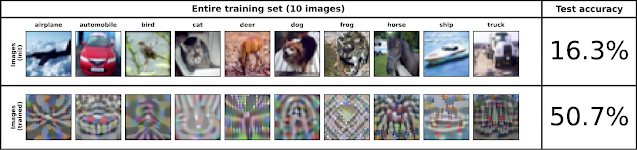
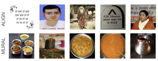
Top: Natural (i.e., unmodified) CIFAR-10 images. Bottom: Distilled dataset (1 image per class) on CIFAR-10 classification task. Using only these 10 synthetic images as training data, a model can achieve test set accuracy of ~51%.

In “Dataset Meta-Learning from Kernel Ridge Regression'', published in ICLR 2021, and “Dataset Distillation with Infinitely Wide Convolutional Networks”, presented at NeurIPS 2021, we introduce two novel dataset distillation algorithms, Kernel Inducing Points (KIP) and Label Solve (LS), which optimize datasets using the loss function arising from kernel regression (a classical machine learning algorithm that fits a linear model to features defined through a kernel). Applying the KIP and LS algorithms, we obtain very efficient distilled datasets for image classification, reducing the datasets to 1, 10, or 50 data points per class while still obtaining state-of-the-art results on a number of benchmark image classification datasets. Additionally, we are also excited to release our distilled datasets to benefit the wider research community.

Methodology
One of the key theoretical insights of deep neural networks (DNN) in recent years has been that increasing the width of DNNs results in more regular behavior that makes them easier to understand. As the width is taken to infinity, DNNs trained by gradient descent converge to the familiar and simpler class of models arising from kernel regression with respect to the neural tangent kernel (NTK), a kernel that measures input similarity by computing dot products of gradients of the neural network. Thanks to the Neural Tangents library, neural kernels for various DNN architectures can be computed in a scalable manner.

We utilized the above infinite-width limit theory of neural networks to tackle dataset distillation. Dataset distillation can be formulated as a two-stage optimization process: an “inner loop” that trains a model on learned data, and an “outer loop” that optimizes the learned data for performance on natural (i.e., unmodified) data. The infinite-width limit replaces the inner loop of training a finite-width neural network with a simple kernel regression. With the addition of a regularizing term, the kernel regression becomes a kernel ridge-regression (KRR) problem. This is a highly valuable outcome because the kernel ridge regressor (i.e., the predictor from the algorithm) has an explicit formula in terms of its training data (unlike a neural network predictor), which means that one can easily optimize the KRR loss function during the outer loop.

The original data labels can be represented by one-hot vectors, i.e., the true label is given a value of 1 and all other labels are given values of 0. Thus, an image of a cat would have the label “cat” assigned a 1 value, while the labels for “dog” and “horse” would be 0. The labels we use involve a subsequent mean-centering step, where we subtract the reciprocal of the number of classes from each component (so 0.1 for 10-way classification) so that the expected value of each label component across the dataset is normalized to zero.

While the labels for natural images appear in this standard form, the labels for our learned distilled datasets are free to be optimized for performance. Having obtained the kernel ridge regressor from the inner loop, the KRR loss function in the outer loop computes the mean-square error between the original labels of natural images and the labels predicted by the kernel ridge regressor. KIP optimizes the support data (images and possibly labels) by minimizing the KRR loss function through gradient-based methods. The Label Solve algorithm directly solves for the set of support labels that minimizes the KRR loss function, generating a unique dense label vector for each (natural) support image.

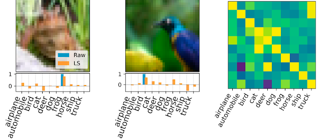
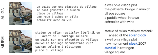
Example of labels obtained by label solving. Left and Middle: Sample images with possible labels listed below. The raw, one-hot label is shown in blue and the final LS generated dense label is shown in orange. Right: The covariance matrix between original labels and learned labels. Here, 500 labels were distilled from the CIFAR-10 dataset. A test accuracy of 69.7% is achieved using these labels for kernel ridge-regression.

Distributed Computation
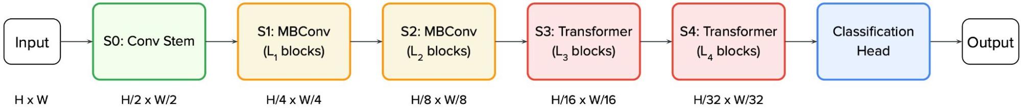
For simplicity, we focus on architectures that consist of convolutional neural networks with pooling layers. Specifically, we focus on the so-called “ConvNet” architecture and its variants because it has been featured in other dataset distillation studies. We used a slightly modified version of ConvNet that has a simple architecture given by three blocks of convolution, ReLu, and 2x2 average pooling and then a final linear readout layer, with an additional 3x3 convolution and ReLu layer prepended (see our GitHub for precise details).

ConvNet architecture used in DC/DSA. Ours has an additional 3x3 Conv and ReLu prepended.

To compute the neural kernels needed in our work, we used the Neural Tangents library.

The first stage of this work, in which we applied KRR, focused on fully-connected networks, whose kernel elements are cheap to compute. But a hurdle facing neural kernels for models with convolutional layers plus pooling is that the computation of each kernel element between two images scales as the square of the number of input pixels (due to the capturing of pixel-pixel correlations by the kernel). So, for the second stage of this work, we needed to distribute the computation of the kernel elements and their gradients across many devices.

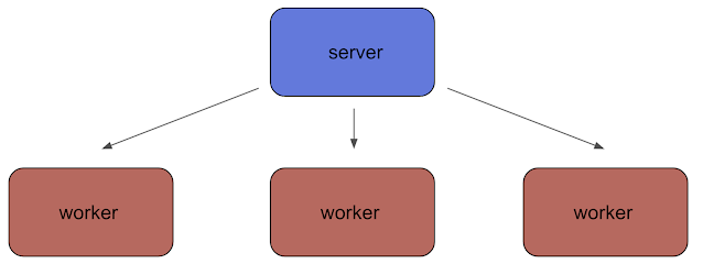
Distributed computation for large scale metalearning.

We invoke a client-server model of distributed computation in which a server distributes independent workloads to a large pool of client workers. A key part of this is to divide the backpropagation step in a way that is computationally efficient (explained in detail in the paper).

We accomplish this using the open-source tools Courier (part of DeepMind’s Launchpad), which allows us to distribute computations across GPUs working in parallel, and JAX, for which novel usage of the jax.vjp function enables computationally efficient gradients. This distributed framework allows us to utilize hundreds of GPUs per distillation of the dataset, for both the KIP and LS algorithms. Given the compute required for such experiments, we are releasing our distilled datasets to benefit the wider research community.

Examples
Our first set of distilled images above used KIP to distill CIFAR-10 down to 1 image per class while keeping the labels fixed. Next, in the below figure, we compare the test accuracy of training on natural MNIST images, KIP distilled images with labels fixed, and KIP distilled images with labels optimized. We highlight that learning the labels provides an effective, albeit mysterious benefit to distilling datasets. Indeed the resulting set of images provides the best test performance (for infinite-width networks) despite being less interpretable.

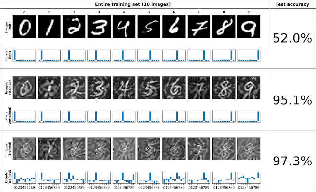
MNIST dataset distillation with trainable and non-trainable labels. Top: Natural MNIST data. Middle: Kernel Inducing Point distilled data with fixed labels. Bottom: Kernel Inducing Point distilled data with learned labels.

Results
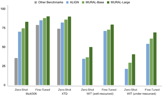
Our distilled datasets achieve state-of-the-art performance on benchmark image classification datasets, improving performance beyond previous state-of-the-art models that used convolutional architectures, Dataset Condensation (DC) and Dataset Condensation with Differentiable Siamese Augmentation (DSA). In particular, for CIFAR-10 classification tasks, a model trained on a dataset consisting of only 10 distilled data entries (1 image / class, 0.02% of the whole dataset) achieves a 64% test set accuracy. Here, learning labels and an additional image preprocessing step leads to a significant increase in performance beyond the 50% test accuracy shown in our first figure (see our paper for details). With 500 images (50 images / class, 1% of the whole dataset), the model reaches 80% test set accuracy. While these numbers are with respect to neural kernels (using the KRR infinite width limit), these distilled datasets can be used to train finite-width neural networks as well. In particular, for 10 data points on CIFAR-10, a finite-width ConvNet neural network achieves 50% test accuracy with 10 images and 68% test accuracy using 500 images, which are still state-of-the-art results. We provide a simple Colab notebook demonstrating this transfer to a finite-width neural network.

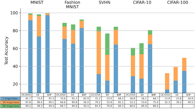
Dataset distillation using Kernel Inducing Points (KIP) with a convolutional architecture outperforms prior state-of-the-art models (DC/DSA) on all benchmark settings on image classification tasks. Label Solve (LS, middle columns) while only distilling information in the labels could often (e.g. CIFAR-10 10, 50 data points per class) outperform prior state-of-the-art models as well.

In some cases, our learned datasets are more effective than a natural dataset one hundred times larger in size.

Conclusion
We believe that our work on dataset distillation opens up many interesting future directions. For instance, our algorithms KIP and LS have demonstrated the effectiveness of using learned labels, an area that remains relatively underexplored. Furthermore, we expect that utilizing efficient kernel approximation methods can help to reduce computational burden and scale up to larger datasets. We hope this work encourages researchers to explore other applications of dataset distillation, including neural architecture search and continual learning, and even potential applications to privacy.

Anyone interested in the KIP and LS learned datasets for further analysis is encouraged to check out our papers [ICLR 2021, NeurIPS 2021] and open-sourced code and datasets available on Github.

Acknowledgement
This project was done in collaboration with Zhourong Chen, Roman Novak and Lechao Xiao. We would like to acknowledge special thanks to Samuel S. Schoenholz, who proposed and helped develop the overall strategy for our distributed KIP learning methodology.


1Now at DeepMind.  

Source: Google AI Blog


Improving Vision Transformer Efficiency and Accuracy by Learning to Tokenize

Transformer models consistently obtain state-of-the-art results in computer vision tasks, including object detection and video classification. In contrast to standard convolutional approaches that process images pixel-by-pixel, the Vision Transformers (ViT) treat an image as a sequence of patch tokens (i.e., a smaller part, or “patch”, of an image made up of multiple pixels). This means that at every layer, a ViT model recombines and processes patch tokens based on relations between each pair of tokens, using multi-head self-attention. In doing so, ViT models have the capability to construct a global representation of the entire image.

At the input-level, the tokens are formed by uniformly splitting the image into multiple segments, e.g., splitting an image that is 512 by 512 pixels into patches that are 16 by 16 pixels. At the intermediate levels, the outputs from the previous layer become the tokens for the next layer. In the case of videos, video ‘tubelets’ such as 16x16x2 video segments (16x16 images over 2 frames) become tokens. The quality and quantity of the visual tokens decide the overall quality of the Vision Transformer.

The main challenge in many Vision Transformer architectures is that they often require too many tokens to obtain reasonable results. Even with 16x16 patch tokenization, for instance, a single 512x512 image corresponds to 1024 tokens. For videos with multiple frames, that results in tens of thousands of tokens needing to be processed at every layer. Considering that the Transformer computation increases quadratically with the number of tokens, this can often make Transformers intractable for larger images and longer videos. This leads to the question: is it really necessary to process that many tokens at every layer?

In “TokenLearner: What Can 8 Learned Tokens Do for Images and Videos?”, an earlier version of which is presented at NeurIPS 2021, we show that adaptively generating a smaller number of tokens, rather than always relying on tokens formed by uniform splitting, enables Vision Transformers to run much faster and perform better. TokenLearner is a learnable module that takes an image-like tensor (i.e., input) and generates a small set of tokens. This module could be placed at various different locations within the model of interest, significantly reducing the number of tokens to be handled in all subsequent layers. The experiments demonstrate that having TokenLearner saves memory and computation by half or more without damaging classification performance, and because of its ability to adapt to inputs, it even increases the accuracy.

The TokenLearner
We implement TokenLearner using a straightforward spatial attention approach. In order to generate each learned token, we compute a spatial attention map highlighting regions-of-importance (using convolutional layers or MLPs). Such a spatial attention map is then applied to the input to weight each region differently (and discard unnecessary regions), and the result is spatially pooled to generate the final learned tokens. This is repeated multiple times in parallel, resulting in a few (~10) tokens out of the original input. This can also be viewed as performing a soft-selection of the pixels based on the weight values, followed by global average pooling. Note that the functions to compute the attention maps are governed by different sets of learnable parameters, and are trained in an end-to-end fashion. This allows the attention functions to be optimized in capturing different spatial information in the input. The figure below illustrates the process.

The TokenLearner module learns to generate a spatial attention map for each output token, and uses it to abstract the input to tokenize. In practice, multiple spatial attention functions are learned, are applied to the input, and generate different token vectors in parallel.

As a result, instead of processing fixed, uniformly tokenized inputs, TokenLearner enables models to process a smaller number of tokens that are relevant to the specific recognition task. That is, (1) we enable adaptive tokenization so that the tokens can be dynamically selected conditioned on the input, and (2) this effectively reduces the total number of tokens, greatly reducing the computation performed by the network. These dynamically and adaptively generated tokens can be used in standard transformer architectures such as ViT for images and ViViT for videos.

Where to Place TokenLearner
After building the TokenLearner module, we had to determine where to place it. We first tried placing it at different locations within the standard ViT architecture with 224x224 images. The number of tokens TokenLearner generated was 8 and 16, much less than 196 or 576 tokens the standard ViTs use. The below figure shows ImageNet few-shot classification accuracies and FLOPS of the models with TokenLearner inserted at various relative locations within ViT B/16, which is the base model with 12 attention layers operating on 16x16 patch tokens.

Top: ImageNet 5-shot transfer accuracy with JFT 300M pre-training, with respect to the relative TokenLearner locations within ViT B/16. Location 0 means TokenLearner is placed before any Transformer layer. Base is the original ViT B/16. Bottom: Computation, measured in terms of billions of floating point operations (GFLOPS), per relative TokenLearner location.

We found that inserting TokenLearner after the initial quarter of the network (at 1/4) achieves almost identical accuracies as the baseline, while reducing the computation to less than a third of the baseline. In addition, placing TokenLearner at the later layer (after 3/4 of the network) achieves even better performance compared to not using TokenLearner while performing faster, thanks to its adaptiveness. Due to the large difference between the number of tokens before and after TokenLearner (e.g., 196 before and 8 after), the relative computation of the transformers after the TokenLearner module becomes almost negligible.

Comparing Against ViTs
We compared the standard ViT models with TokenLearner against those without it while following the same setting on ImageNet few-shot transfer. TokenLearner was placed in the middle of each ViT model at various locations such as at 1/2 and at 3/4. The below figure shows the performance/computation trade-off of the models with and without TokenLearner.

Performance of various versions of ViT models with and without TokenLearner, on ImageNet classification. The models were pre-trained with JFT 300M. The closer a model is to the top-left of each graph the better, meaning that it runs faster and performs better. Observe how TokenLearner models perform better than ViT in terms of both accuracy and computation.

We also inserted TokenLearner within larger ViT models, and compared them against the giant ViT G/14 model. Here, we applied TokenLearner to ViT L/10 and L/8, which are the ViT models with 24 attention layers taking 10x10 (or 8x8) patches as initial tokens. The below figure shows that despite using many fewer parameters and less computation, TokenLearner performs comparably to the giant G/14 model with 48 layers.

Left: Classification accuracy of large-scale TokenLearner models compared to ViT G/14 on ImageNet datasets. Right: Comparison of the number of parameters and FLOPS.

High-Performing Video Models
Video understanding is one of the key challenges in computer vision, so we evaluated TokenLearner on multiple video classification datasets. This was done by adding TokenLearner into Video Vision Transformers (ViViT), which can be thought of as a spatio-temporal version of ViT. TokenLearner learned 8 (or 16) tokens per timestep.

When combined with ViViT, TokenLearner obtains state-of-the-art (SOTA) performance on multiple popular video benchmarks, including Kinetics-400, Kinetics-600, Charades, and AViD, outperforming the previous Transformer models on Kinetics-400 and Kinetics-600 as well as previous CNN models on Charades and AViD.

Models with TokenLearner outperform state-of-the-art on popular video benchmarks (captured from Nov. 2021). Left: popular video classification tasks. Right: comparison to ViViT models.
Visualization of the spatial attention maps in TokenLearner, over time. As the person is moving in the scene, TokenLearner pays attention to different spatial locations to tokenize.

Conclusion
While Vision Transformers serve as powerful models for computer vision, a large number of tokens and their associated computation amount have been a bottleneck for their application to larger images and longer videos. In this project, we illustrate that retaining such a large number of tokens and fully processing them over the entire set of layers is not necessary. Further, we demonstrate that by learning a module that extracts tokens adaptively based on the input image allows attaining even better performance while saving compute. The proposed TokenLearner was particularly effective in video representation learning tasks, which we confirmed with multiple public datasets. A preprint of our work as well as code are publicly available.

Acknowledgement
We thank our co-authors: AJ Piergiovanni, Mostafa Dehghani, and Anelia Angelova. We also thank the Robotics at Google team members for the motivating discussions.

Source: Google AI Blog


MURAL: Multimodal, Multi-task Retrieval Across Languages

For many concepts, there is no direct one-to-one translation from one language to another, and even when there is, such translations often carry different associations and connotations that are easily lost for a non-native speaker. In such cases, however, the meaning may be more obvious when grounded in visual examples. Take, for instance, the word "wedding". In English, one often associates a bride in a white dress and a groom in a tuxedo, but when translated into Hindi (शादी), a more appropriate association may be a bride wearing vibrant colors and a groom wearing a sherwani. What each person associates with the word may vary considerably, but if they are shown an image of the intended concept, the meaning becomes more clear.

The word “wedding” in English and Hindi conveys different mental images. Images are taken from wikipedia, credited to Psoni2402 (left) and David McCandless (right) with CC BY-SA 4.0 license.

With current advances in neural machine translation and image recognition, it is possible to reduce this sort of ambiguity in translation by presenting a text paired with a supporting image. Prior research has made much progress in learning image–text joint representations for high-resource languages, such as English. These representation models strive to encode the image and text into vectors in a shared embedding space, such that the image and the text describing it are close to each other in that space. For example, ALIGN and CLIP have shown that training a dual-encoder model (i.e., one trained with two separate encoders) on image–text pairs using a contrastive learning loss works remarkably well when provided with ample training data.

Unfortunately, such image–text pair data does not exist at the same scale for the majority of languages. In fact, more than 90% of this type of web data belongs to the top-10 highly-resourced languages, such as English and Chinese, with much less data for under-resourced languages. To overcome this issue, one could either try to manually collect image–text pair data for under-resourced languages, which would be prohibitively difficult due to the scale of the undertaking, or one could seek to leverage pre-existing datasets (e.g., translation pairs) that could inform the necessary learned representations for multiple languages.

In “MURAL: Multimodal, Multitask Representations Across Languages”, presented at Findings of EMNLP 2021, we describe a representation model for image–text matching that uses multitask learning applied to image–text pairs in combination with translation pairs covering 100+ languages. This technology could allow users to express words that may not have a direct translation into a target language using images instead. For example, the word “valiha”, refers to a type of tube zither played by the Malagasy people, which lacks a direct translation into most languages, but could be easily described using images. Empirically, MURAL shows consistent improvements over state-of-the-art models, other benchmarks, and competitive baselines across the board. Moreover, MURAL does remarkably well for the majority of the under-resourced languages on which it was tested. Additionally, we discover interesting linguistic correlations learned by MURAL representations.

MURAL Architecture
The MURAL architecture is based on the structure of ALIGN, but employed in a multitask fashion. Whereas ALIGN uses a dual-encoder architecture to draw together representations of images and associated text descriptions, MURAL employs the dual-encoder structure for the same purpose while also extending it across languages by incorporating translation pairs. The dataset of image–text pairs is the same as that used for ALIGN, and the translation pairs are those used for LaBSE.

MURAL solves two contrastive learning tasks: 1) image–text matching and 2) text–text (bitext) matching, with both tasks sharing the text encoder module. The model learns associations between images and text from the image–text data, and learns the representations of hundreds of diverse languages from the translation pairs. The idea is that a shared encoder will transfer the image–text association learned from high-resource languages to under-resourced languages. We find that the best model employs an EfficientNet-B7 image encoder and a BERT-large text encoder, both trained from scratch. The learned representation can be used for downstream visual and vision-language tasks.

The architecture of MURAL depicts dual encoders with a shared text-encoder between the two tasks trained using a contrastive learning loss.

Multilingual Image-to-Text and Text-to-Image Retrieval
To demonstrate MURAL’s capabilities, we choose the task of cross-modal retrieval (i.e., retrieving relevant images given a text and vice versa) and report the scores on various academic image–text datasets covering well-resourced languages, such as MS-COCO (and its Japanese variant, STAIR), Flickr30K (in English) and Multi30K (extended to German, French, Czech), XTD (test-only set with seven well-resourced languages: Italian, Spanish, Russian, Chinese, Polish, Turkish, and Korean). In addition to well-resourced languages, we also evaluate MURAL on the recently published Wikipedia Image–Text (WIT) dataset, which covers 108 languages, with a broad range of both well-resourced (English, French, Chinese, etc.) and under-resourced (Swahili, Hindi, etc.) languages.

MURAL consistently outperforms prior state-of-the-art models, including M3P, UC2, and ALIGN, in both zero-shot and fine-tuned settings evaluated on well-resourced and under-resourced languages. We see remarkable performance gains for under-resourced languages when compared to the state-of-the-art model, ALIGN.

Mean recall on various multilingual image–text retrieval benchmarks. Mean recall is a common metric used to evaluate cross-modal retrieval performance on image–text datasets (higher is better). It measures the Recall@N (i.e., the chance that the ground truth image appears in the first N retrieved images) averaged over six measurements: Image→Text and Text→Image retrieval for N=[1, 5, 10]. Note that XTD scores report Recall@10 for Text→Image retrieval.

Retrieval Analysis
We also analyzed zero-shot retrieved examples on the WIT dataset comparing ALIGN and MURAL for English (en) and Hindi (hi). For under-resourced languages like Hindi, MURAL shows improved retrieval performance compared to ALIGN that reflects a better grasp of the text semantics.

Comparison of the top-5 images retrieved by ALIGN and by MURAL for the Text→Image retrieval task on the WIT dataset for the Hindi text, एक तश्तरी पर बिना मसाले या सब्ज़ी के रखी हुई सादी स्पगॅत्ती”, which translates to the English, “A bowl containing plain noodles without any spices or vegetables”.

Even for Image→Text retrieval in a well-resourced language, like French, MURAL shows better understanding for some words. For example, MURAL returns better results for the query “cadran solaire” (“sundial”, in French) than ALIGN, which doesn’t retrieve any text describing sundials (below).

Comparison of the top-5 text results from ALIGN and from MURAL on the Image→Text retrieval task for the same image of a sundial.

Embeddings Visualization
Previously, researchers have shown that visualizing model embeddings can reveal interesting connections among languages — for instance, representations learned by a neural machine translation (NMT) model have been shown to form clusters based on their membership to a language family. We perform a similar visualization for a subset of languages belonging to the Germanic, Romance, Slavic, Uralic, Finnic, Celtic, and Finno-Ugric language families (widely spoken in Europe and Western Asia). We compare MURAL’s text embeddings with LaBSE’s, which is a text-only encoder.

A plot of LabSE’s embeddings shows distinct clusters of languages influenced by language families. For instance, Romance languages (in purple, below) fall into a different region than Slavic languages (in brown, below). This finding is consistent with prior work that investigates intermediate representations learned by a NMT system.

Visualization of text representations of LaBSE for 35 languages. Languages are color coded based on their genealogical association. Representative languages include: Germanic (red) — German, English, Dutch; Uralic (orange) — Finnish, Estonian; Slavic (brown) — Polish, Russian; Romance (purple) — Italian, Portuguese, Spanish; Gaelic (blue) — Welsh, Irish.

In contrast to LaBSE’s visualization, MURAL’s embeddings, which are learned with a multimodal objective, shows some clusters that are in line with areal linguistics (where elements are shared by languages or dialects in a geographic area) and contact linguistics (where languages or dialects interact and influence each other). Notably, in the MURAL embedding space, Romanian (ro) is closer to the Slavic languages like Bulgarian (bg) and Macedonian (mk), which is in line with the Balkan sprachbund, than it is in LaBSE. Another possible language contact brings Finnic languages, Estonian (et) and Finnish (fi), closer to the Slavic languages cluster. The fact that MURAL pivots on images as well as translations appears to add an additional view on language relatedness as learned in deep representations, beyond the language family clustering observed in a text-only setting.

Visualization of text representations of MURAL for 35 languages. Color coding is the same as the figure above.

Final Remarks
Our findings show that training jointly using translation pairs helps overcome the scarcity of image–text pairs for many under-resourced languages and improves cross-modal performance. Additionally, it is interesting to observe hints of areal linguistics and contact linguistics in the text representations learned by using a multimodal model. This warrants more probing into different connections learned implicitly by multimodal models, such as MURAL. Finally, we hope this work promotes further research in the multimodal, multilingual space where models learn representations of and connections between languages (expressed via images and text), beyond well-resourced languages.

Acknowledgements
This research is in collaboration with Mandy Guo, Krishna Srinivasan, Ting Chen, Sneha Kudugunta, Chao Jia, and Jason Baldridge. We thank Zarana Parekh, Orhan Firat, Yuqing Chen, Apu Shah, Anosh Raj, Daphne Luong, and others who provided feedback for the project. We are also grateful for general support from Google Research teams.

Source: Google AI Blog


Decisiveness in Imitation Learning for Robots

Despite considerable progress in robot learning over the past several years, some policies for robotic agents can still struggle to decisively choose actions when trying to imitate precise or complex behaviors. Consider a task in which a robot tries to slide a block across a table to precisely position it into a slot. There are many possible ways to solve this task, each requiring precise movements and corrections. The robot must commit to just one of these options, but must also be capable of changing plans each time the block ends up sliding farther than expected. Although one might expect such a task to be easy, that is often not the case for modern learning-based robots, which often learn behavior that expert observers describe as indecisive or imprecise.

Example of a baseline explicit behavior cloning model struggling on a task where the robot needs to slide a block across a table and then precisely insert it into a fixture.

To encourage robots to be more decisive, researchers often utilize a discretized action space, which forces the robot to choose option A or option B, without oscillating between options. For example, discretization was a key element of our recent Transporter Networks architecture, and is also inherent in many notable achievements by game-playing agents, such as AlphaGo, AlphaStar, and OpenAI’s Dota bot. But discretization brings its own limitations — for robots that operate in the spatially continuous real world, there are at least two downsides to discretization: (i) it limits precision, and (ii) it triggers the curse of dimensionality, since considering discretizations along many different dimensions can dramatically increase memory and compute requirements. Related to this, in 3D computer vision much recent progress has been powered by continuous, rather than discretized, representations.

With the goal of learning decisive policies without the drawbacks of discretization, today we announce our open source implementation of Implicit Behavioral Cloning (Implicit BC), which is a new, simple approach to imitation learning and was presented last week at CoRL 2021. We found that Implicit BC achieves strong results on both simulated benchmark tasks and on real-world robotic tasks that demand precise and decisive behavior. This includes achieving state-of-the-art (SOTA) results on human-expert tasks from our team’s recent benchmark for offline reinforcement learning, D4RL. On six out of seven of these tasks, Implicit BC outperforms the best previous method for offline RL, Conservative Q Learning. Interestingly, Implicit BC achieves these results without requiring any reward information, i.e., it can use relatively simple supervised learning rather than more-complex reinforcement learning.

Implicit Behavioral Cloning
Our approach is a type of behavior cloning, which is arguably the simplest way for robots to learn new skills from demonstrations. In behavior cloning, an agent learns how to mimic an expert’s behavior using standard supervised learning. Traditionally, behavior cloning involves training an explicit neural network (shown below, left), which takes in observations and outputs expert actions.

The key idea behind Implicit BC is to instead train a neural network to take in both observations and actions, and output a single number that is low for expert actions and high for non-expert actions (below, right), turning behavioral cloning into an energy-based modeling problem. After training, the Implicit BC policy generates actions by finding the action input that has the lowest score for a given observation.

Depiction of the difference between explicit (left) and implicit (right) policies. In the implicit policy, the “argmin” means the action that, when paired with a particular observation, minimizes the value of the energy function.

To train Implicit BC models, we use an InfoNCE loss, which trains the network to output low energy for expert actions in the dataset, and high energy for all others (see below). It is interesting to note that this idea of using models that take in both observations and actions is common in reinforcement learning, but not so in supervised policy learning.

Animation of how implicit models can fit discontinuities — in this case, training an implicit model to fit a step (Heaviside) function. Left: 2D plot fitting the black (X) training points — the colors represent the values of the energies (blue is low, brown is high). Middle: 3D plot of the energy model during training. Right: Training loss curve.

Once trained, we find that implicit models are particularly good at precisely modeling discontinuities (above) on which prior explicit models struggle (as in the first figure of this post), resulting in policies that are newly capable of switching decisively between different behaviors.

But why do conventional explicit models struggle? Modern neural networks almost always use continuous activation functions — for example, Tensorflow, Jax, and PyTorch all only ship with continuous activation functions. In attempting to fit discontinuous data, explicit networks built with these activation functions cannot represent discontinuities, so must draw continuous curves between data points. A key aspect of implicit models is that they gain the ability to represent sharp discontinuities, even though the network itself is composed only of continuous layers.

We also establish theoretical foundations for this aspect, specifically a notion of universal approximation. This proves the class of functions that implicit neural networks can represent, which can help justify and guide future research.

Examples of fitting discontinuous functions, for implicit models (top) compared to explicit models (bottom). The red highlighted insets show that implicit models represent discontinuities (a) and (b) while the explicit models must draw continuous lines (c) and (d) in between the discontinuities.

One challenge faced by our initial attempts at this approach was “high action dimensionality”, which means that a robot must decide how to coordinate many motors all at the same time. To scale to high action dimensionality, we use either autoregressive models or Langevin dynamics.

Highlights
In our experiments, we found Implicit BC does particularly well in the real world, including an order of magnitude (10x) better on the 1mm-precision slide-then-insert task compared to a baseline explicit BC model. On this task the implicit model does several consecutive precise adjustments (below) before sliding the block into place. This task demands multiple elements of decisiveness: there are many different possible solutions due to the symmetry of the block and the arbitrary ordering of push maneuvers, and the robot needs to discontinuously decide when the block has been pushed far “enough” before switching to slide it in a different direction. This is in contrast to the indecisiveness that is often associated with continuous-controlled robots.

Example task of sliding a block across a table and precisely inserting it into a slot. These are autonomous behaviors of our Implicit BC policies, using only images (from the shown camera) as input.
A diverse set of different strategies for accomplishing this task. These are autonomous behaviors from our Implicit BC policies, using only images as input.

In another challenging task, the robot needs to sort blocks by color, which presents a large number of possible solutions due to the arbitrary ordering of sorting. On this task the explicit models are customarily indecisive, while implicit models perform considerably better.

Comparison of implicit (left) and explicit (right) BC models on a challenging continuous multi-item sorting task. (4x speed)

In our testing, implicit BC models can also exhibit robust reactive behavior, even when we try to interfere with the robot, despite the model never seeing human hands.

Robust behavior of the implicit BC model despite interfering with the robot.

Overall, we find that Implicit BC policies can achieve strong results compared to state of the art offline reinforcement learning methods across several different task domains. These results include tasks that, challengingly, have either a low number of demonstrations (as few as 19), high observation dimensionality with image-based observations, and/or high action dimensionality up to 30 — which is a large number of actuators to have on a robot.

Policy learning results of Implicit BC compared to baselines across several domains.

Conclusion
Despite its limitations, behavioral cloning with supervised learning remains one of the simplest ways for robots to learn from examples of human behaviors. As we showed here, replacing explicit policies with implicit policies when doing behavioral cloning allows robots to overcome the "struggle of decisiveness", enabling them to imitate much more complex and precise behaviors. While the focus of our results here was on robot learning, the ability of implicit functions to model sharp discontinuities and multimodal labels may have broader interest in other application domains of machine learning as well.

Acknowledgements
Pete and Corey summarized research performed together with other co-authors: Andy Zeng, Oscar Ramirez, Ayzaan Wahid, Laura Downs, Adrian Wong, Johnny Lee, Igor Mordatch, and Jonathan Tompson. The authors would also like to thank Vikas Sindwhani for project direction advice; Steve Xu, Robert Baruch, Arnab Bose for robot software infrastructure; Jake Varley, Alexa Greenberg for ML infrastructure; and Kamyar Ghasemipour, Jon Barron, Eric Jang, Stephen Tu, Sumeet Singh, Jean-Jacques Slotine, Anirudha Majumdar, Vincent Vanhoucke for helpful feedback and discussions.

Source: Google AI Blog


MetNet-2: Deep Learning for 12-Hour Precipitation Forecasting

Deep learning has successfully been applied to a wide range of important challenges, such as cancer prevention and increasing accessibility. The application of deep learning models to weather forecasts can be relevant to people on a day-to-day basis, from helping people plan their day to managing food production, transportation systems, or the energy grid. Weather forecasts typically rely on traditional physics-based techniques powered by the world’s largest supercomputers. Such methods are constrained by high computational requirements and are sensitive to approximations of the physical laws on which they are based.

Deep learning offers a new approach to computing forecasts. Rather than incorporating explicit physical laws, deep learning models learn to predict weather patterns directly from observed data and are able to compute predictions faster than physics-based techniques. These approaches also have the potential to increase the frequency, scope, and accuracy of the predicted forecasts.

Illustration of the computation through MetNet-2. As the computation progresses, the network processes an ever larger context from the input and makes a probabilistic forecast of the likely future weather conditions.

Within weather forecasting, deep learning techniques have shown particular promise for nowcasting — i.e., predicting weather up to 2-6 hours ahead. Previous work has focused on using direct neural network models for weather data, extending neural forecasts from 0 to 8 hours with the MetNet architecture, generating continuations of radar data for up to 90 minutes ahead, and interpreting the weather information learned by these neural networks. Still, there is an opportunity for deep learning to extend improvements to longer-range forecasts.

To that end, in “Skillful Twelve Hour Precipitation Forecasts Using Large Context Neural Networks”, we push the forecasting boundaries of our neural precipitation model to 12 hour predictions while keeping a spatial resolution of 1 km and a time resolution of 2 minutes. By quadrupling the input context, adopting a richer weather input state, and extending the architecture to capture longer-range spatial dependencies, MetNet-2 substantially improves on the performance of its predecessor, MetNet. Compared to physics-based models, MetNet-2 outperforms the state-of-the-art HREF ensemble model for weather forecasts up to 12 hours ahead.

MetNet-2 Features and Architecture
Neural weather models like MetNet-2 map observations of the Earth to the probability of weather events, such as the likelihood of rain over a city in the afternoon, of wind gusts reaching 20 knots, or of a sunny day ahead. End-to-end deep learning has the potential to both streamline and increase quality by directly connecting a system's inputs and outputs. With this in mind, MetNet-2 aims to minimize both the complexity and the total number of steps involved in creating a forecast.

The inputs to MetNet-2 include the radar and satellite images also used in MetNet. To capture a more comprehensive snapshot of the atmosphere with information such as temperature, humidity, and wind direction — critical for longer forecasts of up to 12 hours — MetNet-2 also uses the pre-processed starting state used in physical models as a proxy for this additional weather information. The radar-based measures of precipitation (MRMS) serve as the ground truth (i.e., what we are trying to predict) that we use in training to optimize MetNet-2’s parameters.

Example ground truth image: Instantaneous precipitation (mm/hr) based on radar (MRMS) capturing a 12 hours-long progression.

MetNet-2’s probabilistic forecasts can be viewed as averaging all possible future weather conditions weighted by how likely they are. Due to its probabilistic nature, MetNet-2 can be likened to physics-based ensemble models, which average some number of future weather conditions predicted by a variety of physics-based models. One notable difference between these two approaches is the duration of the core part of the computation: ensemble models take ~1 hour, whereas MetNet-2 takes ~1 second.

Steps in a MetNet-2 forecast and in a physics-based ensemble.

One of the main challenges that MetNet-2 must overcome to make 12 hour long forecasts is capturing a sufficient amount of spatial context in the input images. For each additional forecast hour we include 64 km of context in every direction at the input. This results in an input context of size 20482 km2 — four times that used in MetNet. In order to process such a large context, MetNet-2 employs model parallelism whereby the model is distributed across 128 cores of a Cloud TPU v3-128. Due to the size of the input context, MetNet-2 replaces the attentional layers of MetNet with computationally more efficient convolutional layers. But standard convolutional layers have local receptive fields that may fail to capture large spatial contexts, so MetNet-2 uses dilated receptive fields, whose size doubles layer after layer, in order to connect points in the input that are far apart one from the other.

Example of input spatial context and target area for MetNet-2.

Results
Because MetNet-2’s predictions are probabilistic, the model’s output is naturally compared with the output of similarly probabilistic ensemble or post-processing models. HREF is one such state-of-the-art ensemble model for precipitation in the United States, which aggregates ten predictions from five different models, twice a day. We evaluate the forecasts using established metrics, such as the Continuous Ranked Probability Score, which captures the magnitude of the probabilistic error of a model’s forecasts relative to the ground truth observations. Despite not performing any physics-based calculations, MetNet-2 is able to outperform HREF up to 12 hours into the future for both low and high levels of precipitation.

Continuous Ranked Probability Score (CRPS; lower is better) for MetNet-2 vs HREF aggregated over a large number of test patches randomly located in the Continental United States.

Examples of Forecasts
The following figures provide a selection of forecasts from MetNet-2 compared with the physics-based ensemble HREF and the ground truth MRMS.

Probability maps for the cumulative precipitation rate of 1 mm/hr on January 3, 2019 over the Pacific NorthWest. The maps are shown for each hour of lead time from 1 to 12. Left: Ground truth, source MRMS. Center: Probability map as predicted by MetNet-2 . Right: Probability map as predicted by HREF.
Comparison of 0.2 mm/hr precipitation on March 30, 2020 over Denver, Colorado. Left: Ground truth, source MRMS. Center: Probability map as predicted by MetNet-2 . Right: Probability map as predicted by HREF.MetNet-2 is able to predict the onset of the storm (called convective initiation) earlier in the forecast than HREF as well as the storm’s starting location, whereas HREF misses the initiation location, but captures its growth phase well.
Comparison of 2 mm/hr precipitation stemming from Hurricane Isaias, an extreme weather event that occurred on August 4, 2020 over the North East coast of the US. Left: Ground truth, source MRMS. Center: Probability map as predicted by MetNet-2. Right: Probability map as predicted by HREF.

Interpreting What MetNet-2 Learns About Weather
Because MetNet-2 does not use hand-crafted physical equations, its performance inspires a natural question: What kind of physical relations about the weather does it learn from the data during training? Using advanced interpretability tools, we further trace the impact of various input features on MetNet-2’s performance at different forecast timelines. Perhaps the most surprising finding is that MetNet-2 appears to emulate the physics described by Quasi-Geostrophic Theory, which is used as an effective approximation of large-scale weather phenomena. MetNet-2 was able to pick up on changes in the atmospheric forces, at the scale of a typical high- or low-pressure system (i.e., the synoptic scale), that bring about favorable conditions for precipitation, a key tenet of the theory.

Conclusion
MetNet-2 represents a step toward enabling a new modeling paradigm for weather forecasting that does not rely on hand-coding the physics of weather phenomena, but rather embraces end-to-end learning from observations to weather targets and parallel forecasting on low-precision hardware. Yet many challenges remain on the path to fully achieving this goal, including incorporating more raw data about the atmosphere directly (rather than using the pre-processed starting state from physical models), broadening the set of weather phenomena, increasing the lead time horizon to days and weeks, and widening the geographic coverage beyond the United States.

Acknowledgements
Shreya Agrawal, Casper Sønderby, Manoj Kumar, Jonathan Heek, Carla Bromberg, Cenk Gazen, Jason Hickey, Aaron Bell, Marcin Andrychowicz, Amy McGovern, Rob Carver, Stephan Hoyer, Zack Ontiveros, Lak Lakshmanan, David McPeek, Ian Gonzalez, Claudio Martella, Samier Merchant, Fred Zyda, Daniel Furrer and Tom Small.


Source: Google AI Blog


Deciding Which Tasks Should Train Together in Multi-Task Neural Networks

Many machine learning (ML) models typically focus on learning one task at a time. For example, language models predict the probability of a next word given a context of past words, and object detection models identify the object(s) that are present in an image. However, there may be instances when learning from many related tasks at the same time would lead to better modeling performance. This is addressed in the domain of multi-task learning, a subfield of ML in which multiple objectives are trained within the same model at the same time.

Consider a real-world example: the game of ping-pong. When playing ping-pong, it is often advantageous to judge the distance, spin, and imminent trajectory of the ping-pong ball to adjust your body and line up a swing. While each of these tasks are unique — predicting the spin of a ping-pong ball is fundamentally distinct from predicting its location — improving your reasoning of the location and spin of the ball will likely help you better predict its trajectory and vice-versa. By analogy, within the realm of deep learning, training a model to predict three related tasks (i.e., the location, spin, and trajectory of a ping-pong ball) may result in improved performance over a model that only predicts a single objective.

Left: Three single-task networks, each of which uses the same input to predict the spin, distance, or trajectory of the ping-pong ball, respectively. Right: A single multi-task network that simultaneously predicts the spin, distance, and trajectory.

In “Efficiently Identifying Task Groupings in Multi-Task Learning”, a spotlight presentation at NeurIPS 2021, we describe a method called Task Affinity Groupings (TAG) that determines which tasks should be trained together in multi-task neural networks. Our approach attempts to divide a set of tasks into smaller subsets such that the performance across all tasks is maximized. To accomplish this goal, it trains all tasks together in a single multi-task model and measures the degree to which one task’s gradient update on the model’s parameters would affect the loss of the other tasks in the network. We denote this quantity as inter-task affinity. Our experimental findings indicate that selecting groups of tasks that maximize inter-task affinity correlates strongly with overall model performance.

Which Tasks Should Train Together?
In the ideal case, a multi-task learning model will apply the information it learns during training on one task to decrease the loss on other tasks included in training the network. This transfer of information leads to a single model that can not only make multiple predictions, but may also exhibit improved accuracy for those predictions when compared with the performance of training a different model for each task. On the other hand, training a single model on many tasks may lead to competition for model capacity and severely degrade performance. This latter scenario often occurs when tasks are unrelated. Returning to our ping-pong analogy, imagine trying to predict the location, spin, and trajectory of the ping-pong ball while simultaneously recounting the Fibonnaci sequence. Not a fun prospect, and most likely detrimental to your progression as a ping-pong player.

One direct approach to select the subset of tasks on which a model should train is to perform an exhaustive search over all possible combinations of multi-task networks for a set of tasks. However, the cost associated with this search can be prohibitive, especially when there are a large number of tasks, because the number of possible combinations increases exponentially with respect to the number of tasks in the set. This is further complicated by the fact that the set of tasks to which a model is applied may change throughout its lifetime. As tasks are added to or dropped from the set of all tasks, this costly analysis would need to be repeated to determine new groupings. Moreover, as the scale and complexity of models continues to increase, even approximate task grouping algorithms that evaluate only a subset of possible multi-task networks may become prohibitively costly and time-consuming to evaluate.

Building Task Affinity Groupings
In examining this challenge, we drew inspiration from meta-learning, a domain of machine learning that trains a neural network that can be quickly adapted to a new, and previously unseen task. One of the classic meta-learning algorithms, MAML, applies a gradient update to the models’ parameters for a collection of tasks and then updates its original set of parameters to minimize the loss for a subset of tasks in that collection computed at the updated parameter values. Using this method, MAML trains the model to learn representations that will not minimize the loss for its current set of weights, but rather for the weights after one or more steps of training. As a result, MAML trains a models’ parameters to have the capacity to quickly adapt to a previously unseen task because it optimizes for the future, not the present.

TAG employs a similar mechanism to gain insight into the training dynamics of multi-task neural networks. In particular, it updates the model’s parameters with respect only to a single task, looks at how this change would affect the other tasks in the multi-task neural network, and then undoes this update. This process is then repeated for every other task to gather information on how each task in the network would interact with any other task. Training then continues as normal by updating the model’s shared parameters with respect to every task in the network.

Collecting these statistics, and looking at their dynamics throughout training, reveals that certain tasks consistently exhibit beneficial relationships, while some are antagonistic towards each other. A network selection algorithm can leverage this data in order to group tasks together that maximize inter-task affinity, subject to a practitioner’s choice of how many multi-task networks can be used during inference.

Overview of TAG. First, tasks are trained together in the same network while computing inter-task affinities. Second, the network selection algorithm finds task groupings that maximize inter-task affinity. Third, the resulting multi-task networks are trained and deployed.

Results
Our experimental findings indicate that TAG can select very strong task groupings. On the CelebA and Taskonomy datasets, TAG is competitive with the prior state-of-the-art, while operating between 32x and 11.5x faster, respectively. On the Taskonomy dataset, this speedup translates to 2,008 fewer Tesla V100 GPU hours to find task groupings.

Conclusion
TAG is an efficient method to determine which tasks should train together in a single training run. The method looks at how tasks interact through training, notably, the effect that updating the model’s parameters when training on one task would have on the loss values of the other tasks in the network. We find that selecting groups of tasks to maximize this score correlates strongly with model performance.

Acknowledgements
We would like to thank Ehsan Amid, Zhe Zhao, Tianhe Yu, Rohan Anil, and Chelsea Finn for their fundamental contributions to this work. We also recognize Tom Small for designing the animation, and Google Research as a whole for fostering a collaborative and uplifting research environment.

Source: Google AI Blog


Pathdreamer: A World Model for Indoor Navigation

When a person navigates around an unfamiliar building, they take advantage of many visual, spatial and semantic cues to help them efficiently reach their goal. For example, even in an unfamiliar house, if they see a dining area, they can make intelligent predictions about the likely location of the kitchen and lounge areas, and therefore the expected location of common household objects. For robotic agents, taking advantage of semantic cues and statistical regularities in novel buildings is challenging. A typical approach is to implicitly learn what these cues are, and how to use them for navigation tasks, in an end-to-end manner via model-free reinforcement learning. However, navigation cues learned in this way are expensive to learn, hard to inspect, and difficult to re-use in another agent without learning again from scratch.

People navigating in unfamiliar buildings can take advantage of visual, spatial and semantic cues to predict what’s around a corner. A computational model with this capability is a visual world model.

An appealing alternative for robotic navigation and planning agents is to use a world model to encapsulate rich and meaningful information about their surroundings, which enables an agent to make specific predictions about actionable outcomes within their environment. Such models have seen widespread interest in robotics, simulation, and reinforcement learning with impressive results, including finding the first known solution for a simulated 2D car racing task, and achieving human-level performance in Atari games. However, game environments are still relatively simple compared to the complexity and diversity of real-world environments.

In “Pathdreamer: A World Model for Indoor Navigation”, published at ICCV 2021, we present a world model that generates high-resolution 360º visual observations of areas of a building unseen by an agent, using only limited seed observations and a proposed navigation trajectory. As illustrated in the video below, the Pathdreamer model can synthesize an immersive scene from a single viewpoint, predicting what an agent might see if it moved to a new viewpoint or even a completely unseen area, such as around a corner. Beyond potential applications in video editing and bringing photos to life, solving this task promises to codify knowledge about human environments to benefit robotic agents navigating in the real world. For example, a robot tasked with finding a particular room or object in an unfamiliar building could perform simulations using the world model to identify likely locations before physically searching anywhere. World models such as Pathdreamer can also be used to increase the amount of training data for agents, by training agents in the model.

Provided with just a single observation (RGB, depth, and segmentation) and a proposed navigation trajectory as input, Pathdreamer synthesizes high resolution 360º observations up to 6-7 meters away from the original location, including around corners. For more results, please refer to the full video.

How Does Pathdreamer Work?
Pathdreamer takes as input a sequence of one or more previous observations, and generates predictions for a trajectory of future locations, which may be provided up front or iteratively by the agent interacting with the returned observations. Both inputs and predictions consist of RGB, semantic segmentation, and depth images. Internally, Pathdreamer uses a 3D point cloud to represent surfaces in the environment. Points in the cloud are labelled with both their RGB color value and their semantic segmentation class, such as wall, chair or table.

To predict visual observations in a new location, the point cloud is first re-projected into 2D at the new location to provide ‘guidance’ images, from which Pathdreamer generates realistic high-resolution RGB, semantic segmentation and depth. As the model ‘moves’, new observations (either real or predicted) are accumulated in the point cloud. One advantage of using a point cloud for memory is temporal consistency — revisited regions are rendered in a consistent manner to previous observations.

Internally, Pathdreamer represents surfaces in the environment via a 3D point cloud containing both semantic labels (top) and RGB color values (bottom). To generate a new observation, Pathdreamer ‘moves’ through the point cloud to the new location and uses the re-projected point cloud image for guidance.

To convert guidance images into plausible, realistic outputs Pathdreamer operates in two stages: the first stage, the structure generator, creates segmentation and depth images, and the second stage, the image generator, renders these into RGB outputs. Conceptually, the first stage provides a plausible high-level semantic representation of the scene, and the second stage renders this into a realistic color image. Both stages are based on convolutional neural networks.

Pathdreamer operates in two stages: the first stage, the structure generator, creates segmentation and depth images, and the second stage, the image generator, renders these into RGB outputs. The structure generator is conditioned on a noise variable to enable the model to synthesize diverse scenes in areas of high uncertainty.

Diverse Generation Results
In regions of high uncertainty, such as an area predicted to be around a corner or in an unseen room, many different scenes are possible. Incorporating ideas from stochastic video generation, the structure generator in Pathdreamer is conditioned on a noise variable, which represents the stochastic information about the next location that is not captured in the guidance images. By sampling multiple noise variables, Pathdreamer can synthesize diverse scenes, allowing an agent to sample multiple plausible outcomes for a given trajectory. These diverse outputs are reflected not only in the first stage outputs (semantic segmentation and depth images), but in the generated RGB images as well.

Pathdreamer is capable of generating multiple diverse and plausible images for regions of high uncertainty. Guidance images on the leftmost column represent pixels that were previously seen by the agent. Black pixels represent regions that were previously unseen, for which Pathdreamer renders diverse outputs by sampling multiple random noise vectors. In practice, the generated output can be informed by new observations as the agent navigates the environment.

Pathdreamer is trained with images and 3D environment reconstructions from Matterport3D, and is capable of synthesizing realistic images as well as continuous video sequences. Because the output imagery is high-resolution and 360º, it can be readily converted for use by existing navigation agents for any camera field of view. For more details and to try out Pathdreamer yourself, we recommend taking a look at our open source code.

Application to Visual Navigation Tasks
As a visual world model, Pathdreamer shows strong potential to improve performance on downstream tasks. To demonstrate this, we apply Pathdreamer to the task of Vision-and-Language Navigation (VLN), in which an embodied agent must follow a natural language instruction to navigate to a location in a realistic 3D environment. Using the Room-to-Room (R2R) dataset, we conduct an experiment in which an instruction-following agent plans ahead by simulating many possible navigable trajectory through the environment, ranking each against the navigation instructions, and choosing the best ranked trajectory to execute. Three settings are considered. In the Ground-Truth setting, the agent plans by interacting with the actual environment, i.e. by moving. In the Baseline setting, the agent plans ahead without moving by interacting with a navigation graph that encodes the navigable routes within the building, but does not provide any visual observations. In the Pathdreamer setting, the agent plans ahead without moving by interacting with the navigation graph and also receives corresponding visual observations generated by Pathdreamer.

When planning ahead for three steps (approximately 6m), in the Pathdreamer setting the VLN agent achieves a navigation success rate of 50.4%, significantly higher than the 40.6% success rate in the Baseline setting without Pathdreamer. This suggests that Pathdreamer encodes useful and accessible visual, spatial and semantic knowledge about real-world indoor environments. As an upper bound illustrating the performance of a perfect world model, under the Ground-Truth setting (planning by moving) the agent’s success rate is 59%, although we note that this setting requires the agent to expend significant time and resources to physically explore many trajectories, which would likely be prohibitively costly in a real-world setting.

We evaluate several planning settings for an instruction-following agent using the Room-to-Room (R2R) dataset. Planning ahead using a navigation graph with corresponding visual observations synthesized by Pathdreamer (Pathdreamer setting) is more effective than planning ahead using the navigation graph alone (Baseline setting), capturing around half the benefit of planning ahead using a world model that perfectly matches reality (Ground-Truth setting).

Conclusions and Future Work
These results showcase the promise of using world models such as Pathdreamer for complicated embodied navigation tasks. We hope that Pathdreamer will help unlock model-based approaches to challenging embodied navigation tasks such as navigating to specified objects and VLN.

Applying Pathdreamer to other embodied navigation tasks such as Object-Nav, continuous VLN, and street-level navigation are natural directions for future work. We also envision further research on improved architecture and modeling directions for the Pathdreamer model, as well as testing it on more diverse datasets, including but not limited to outdoor environments. To explore Pathdreamer in more detail, please visit our GitHub repository.

Acknowledgements
This project is a collaboration with Jason Baldridge, Honglak Lee, and Yinfei Yang. We thank Austin Waters, Noah Snavely, Suhani Vora, Harsh Agrawal, David Ha, and others who provided feedback throughout the project. We are also grateful for general support from Google Research teams. Finally, we thank Tom Small for creating the animation in the third figure.

Source: Google AI Blog


Toward Fast and Accurate Neural Networks for Image Recognition

As neural network models and training data size grow, training efficiency is becoming an important focus for deep learning. For example, GPT-3 demonstrates remarkable capability in few-shot learning, but it requires weeks of training with thousands of GPUs, making it difficult to retrain or improve. What if, instead, one could design neural networks that were smaller and faster, yet still more accurate?

In this post, we introduce two families of models for image recognition that leverage neural architecture search, and a principled design methodology based on model capacity and generalization. The first is EfficientNetV2 (accepted at ICML 2021), which consists of convolutional neural networks that aim for fast training speed for relatively small-scale datasets, such as ImageNet1k (with 1.28 million images). The second family is CoAtNet, which are hybrid models that combine convolution and self-attention, with the goal of achieving higher accuracy on large-scale datasets, such as ImageNet21 (with 13 million images) and JFT (with billions of images). Compared to previous results, our models are 4-10x faster while achieving new state-of-the-art 90.88% top-1 accuracy on the well-established ImageNet dataset. We are also releasing the source code and pretrained models on the Google AutoML github.

EfficientNetV2: Smaller Models and Faster Training
EfficientNetV2 is based upon the previous EfficientNet architecture. To improve upon the original, we systematically studied the training speed bottlenecks on modern TPUs/GPUs and found: (1) training with very large image sizes results in higher memory usage and thus is often slower on TPUs/GPUs; (2) the widely used depthwise convolutions are inefficient on TPUs/GPUs, because they exhibit low hardware utilization; and (3) the commonly used uniform compound scaling approach, which scales up every stage of convolutional networks equally, is sub-optimal. To address these issues, we propose both a training-aware neural architecture search (NAS), in which the training speed is included in the optimization goal, and a scaling method that scales different stages in a non-uniform manner.

The training-aware NAS is based on the previous platform-aware NAS, but unlike the original approach, which mostly focuses on inference speed, here we jointly optimize model accuracy, model size, and training speed. We also extend the original search space to include more accelerator-friendly operations, such as FusedMBConv, and simplify the search space by removing unnecessary operations, such as average pooling and max pooling, which are never selected by NAS. The resulting EfficientNetV2 networks achieve improved accuracy over all previous models, while being much faster and up to 6.8x smaller.

To further speed up the training process, we also propose an enhanced method of progressive learning, which gradually changes image size and regularization magnitude during training. Progressive training has been used in image classification, GANs, and language models. This approach focuses on image classification, but unlike previous approaches that often trade accuracy for improved training speed, can slightly improve the accuracy while also significantly reducing training time. The key idea in our improved approach is to adaptively change regularization strength, such as dropout ratio or data augmentation magnitude, according to the image size. For the same network, small image size leads to lower network capacity and thus requires weak regularization; vice versa, a large image size requires stronger regularization to combat overfitting.

Progressive learning for EfficientNetV2. Here we mainly focus on three types of regularizations: data augmentation, mixup, and dropout.

We evaluate the EfficientNetV2 models on ImageNet and a few transfer learning datasets, such as CIFAR-10/100, Flowers, and Cars. On ImageNet, EfficientNetV2 significantly outperforms previous models with about 5–11x faster training speed and up to 6.8x smaller model size, without any drop in accuracy.

EfficientNetV2 achieves much better training efficiency than prior models for ImageNet classification.

CoAtNet: Fast and Accurate Models for Large-Scale Image Recognition
While EfficientNetV2 is still a typical convolutional neural network, recent studies on Vision Transformer (ViT) have shown that attention-based transformer models could perform better than convolutional neural networks on large-scale datasets like JFT-300M. Inspired by this observation, we further expand our study beyond convolutional neural networks with the aim of finding faster and more accurate vision models.

In “CoAtNet: Marrying Convolution and Attention for All Data Sizes”, we systematically study how to combine convolution and self-attention to develop fast and accurate neural networks for large-scale image recognition. Our work is based on an observation that convolution often has better generalization (i.e., the performance gap between training and evaluation) due to its inductive bias, while self-attention tends to have greater capacity (i.e., the ability to fit large-scale training data) thanks to its global receptive field. By combining convolution and self-attention, our hybrid models can achieve both better generalization and greater capacity.

Comparison between convolution, self-attention, and hybrid models. Convolutional models converge faster, ViTs have better capacity, while the hybrid models achieve both faster convergence and better accuracy.

We observe two key insights from our study: (1) depthwise convolution and self-attention can be naturally unified via simple relative attention, and (2) vertically stacking convolution layers and attention layers in a way that considers their capacity and computation required in each stage (resolution) is surprisingly effective in improving generalization, capacity and efficiency. Based on these insights, we have developed a family of hybrid models with both convolution and attention, named CoAtNets (pronounced “coat” nets). The following figure shows the overall CoAtNet network architecture:

Overall CoAtNet architecture. Given an input image with size HxW, we first apply convolutions in the first stem stage (S0) and reduce the size to H/2 x W/2. The size continues to reduce with each stage. Ln refers to the number of layers. Then, the early two stages (S1 and S2) mainly adopt MBConv building blocks consisting of depthwise convolution. The later two stages (S3 and S4) mainly adopt Transformer blocks with relative self-attention. Unlike the previous Transformer blocks in ViT, here we use pooling between stages, similar to Funnel Transformer. Finally, we apply a classification head to generate class prediction.

CoAtNet models consistently outperform ViT models and its variants across a number of datasets, such as ImageNet1K, ImageNet21K, and JFT. When compared to convolutional networks, CoAtNet exhibits comparable performance on a small-scale dataset (ImageNet1K) and achieves substantial gains as the data size increases (e.g. on ImageNet21K and JFT).

Comparison between CoAtNet and previous models after pre-training on the medium sized ImageNet21K dataset. Under the same model size, CoAtNet consistently outperforms both ViT and convolutional models. Noticeably, with only ImageNet21K, CoAtNet is able to match the performance of ViT-H pre-trained on JFT.

We also evaluated CoAtNets on the large-scale JFT dataset. To reach a similar accuracy target, CoAtNet trains about 4x faster than previous ViT models and more importantly, achieves a new state-of-the-art top-1 accuracy on ImageNet of 90.88%.

Comparison between CoAtNets and previous ViTs. ImageNet top-1 accuracy after pre-training on JFT dataset under different training budget. The four best models are trained on JFT-3B with about 3 billion images.

Conclusion and Future Work
In this post, we introduce two families of neural networks, named EfficientNetV2 and CoAtNet, which achieve state-of-the-art performance on image recognition. All EfficientNetV2 models are open sourced and the pretrained models are also available on the TFhub. CoAtNet models will also be open-sourced soon. We hope these new neural networks can benefit the research community and the industry. In the future we plan to further optimize these models and apply them to new tasks, such as zero-shot learning and self-supervised learning, which often require fast models with high capacity.

Acknowledgements
Special thanks to our co-authors Hanxiao Liu and Quoc Le. We also thank the Google Research, Brain Team and the open source contributors.

Source: Google AI Blog


Revisiting Mask-Head Architectures for Novel Class Instance Segmentation

Instance segmentation is the task of grouping pixels in an image into instances of individual things, and identifying those things with a class label (countable objects such as people, animals, cars, etc., and assigning unique identifiers to each, e.g., car_1 and car_2). As a core computer vision task, it is critical to many downstream applications, such as self-driving cars, robotics, medical imaging, and photo editing. In recent years, deep learning has made significant strides in solving the instance segmentation problem with architectures like Mask R-CNN. However, these methods rely on collecting a large labeled instance segmentation dataset. But unlike bounding box labels, which can be collected in 7 seconds per instance with methods like Extreme clicking, collecting instance segmentation labels (called “masks”) can take up to 80 seconds per instance, an effort that is costly and creates a high barrier to entry for this research. And a related task, pantopic segmentation, requires even more labeled data.

The partially supervised instance segmentation setting, where only a small set of classes are labeled with instance segmentation masks and the remaining (majority of) classes are labeled only with bounding boxes, is an approach that has the potential to reduce the dependence on manually-created mask labels, thereby significantly lowering the barriers to developing an instance segmentation model. However this partially supervised approach also requires a stronger form of model generalization to handle novel classes not seen at training time—e.g., training with only animal masks and then tasking the model to produce accurate instance segmentations for buildings or plants. Further, naïve approaches, such as training a class-agnostic Mask R-CNN, while ignoring mask losses for any instances that don’t have mask labels, have not worked well. For example, on the typical “VOC/Non-VOC” benchmark, where one trains on masks for a subset of 20 classes in COCO (called “seen classes”) and is tested on the remaining 60 classes (called “unseen classes”), a typical Mask R-CNN with Resnet-50 backbone gets to only ~18% mask mAP (mean Average Precision, higher is better) on unseen classes, whereas when fully supervised it can achieve a much higher >34% mask mAP on the same set.

In “The surprising impact of mask-head architecture on novel class segmentation”, to be presented at ICCV 2021, we identify the main culprits for Mask R-CNN’s poor performance on novel classes and propose two easy-to-implement fixes (one training protocol fix, one mask-head architecture fix) that work in tandem to close the gap to fully supervised performance. We show that our approach applies generally to crop-then-segment models, i.e., a Mask R-CNN or Mask R-CNN-like architecture that computes a feature representation of the entire image and then subsequently passes per-instance crops to a second-stage mask prediction network—also called a mask-head network. Putting our findings together, we propose a Mask R-CNN–based model that improves over the current state-of-the-art by a significant 4.7% mask mAP without requiring more complex auxiliary loss functions, offline trained priors, or weight transfer functions proposed by previous work. We have also open sourced the code bases for two versions of the model, called Deep-MAC and Deep-MARC, and published a colab to interactively produce masks like the video demo below.

A demo of our model, DeepMAC, which learns to predict accurate masks, given user specified boxes, even on novel classes that were not seen at training time. Try it yourself in the colab. Image credits: Chris Briggs, Wikipedia and Europeana.

Impact of Cropping Methodology in Partially Supervised Settings
An important step of crop-then-segment models is cropping—Mask R-CNN is trained by cropping a feature map as well as the ground truth mask to a bounding box corresponding to each instance. These cropped features are passed to another neural network (called a mask-head network) that computes a final mask prediction, which is then compared against the ground truth crop in the mask loss function. There are two choices for cropping: (1) cropping directly to the ground truth bounding box of an instance, or (2) cropping to bounding boxes predicted by the model (called, proposals). At test time, cropping is always performed with proposals as ground truth boxes are not assumed to be available.

Cropping to ground truth boxes vs. cropping to proposals predicted by a model during training. Standard Mask R-CNN implementations use both types of crops, but we show that cropping exclusively to ground truth boxes yields significantly stronger performance on novel categories.
We consider a general family of Mask R-CNN–like architectures with one small, but critical difference from typical Mask R-CNN training setups: we crop using ground truth boxes (instead of proposal boxes) at training time.

Typical Mask R-CNN implementations pass both types of crops to the mask head. However, this choice has traditionally been considered an unimportant implementation detail, because it does not affect performance significantly in the fully supervised setting. In contrast, for partially supervised settings, we find that cropping methodology plays a significant role—while cropping exclusively to ground truth boxes during training doesn’t change the results significantly in the fully supervised setting, it has a surprising and dramatic positive impact in the partially supervised setting, performing significantly better on unseen classes.

Performance of Mask R-CNN on unseen classes when trained with either proposals and ground truth (the default) or with only ground truth boxes. Training mask heads with only ground truth boxes yields a significant boost to performance on unseen classes, upwards of 9% mAP. We report performance with the ResNet-101-FPN backbone.

Unlocking the Full Generalization Potential of the Mask Head
Even more surprisingly, the above approach unlocks a novel phenomenon—with cropping-to-ground truth enabled during training, the mask head of Mask R-CNN takes on a disproportionate role in the ability of the model to generalize to unseen classes. As an example, in the following figure, we compare models that all have cropping-to-ground-truth enabled, but different out-of-the-box mask-head architectures on a parking meter, cell phone, and pizza (classes unseen during training).

Mask predictions for unseen classes with four different mask-head architectures (from left to right: ResNet-4, ResNet-12, ResNet-20, Hourglass-20, where the number refers to the number of layers of the neural network). Despite never having seen masks from the ‘parking meter’, ‘pizza’ or ‘mobile phone’ class, the rightmost mask-head architecture can segment these classes correctly. From left to right, we show better mask-head architectures predicting better masks. Moreover, this difference is only apparent when evaluating on unseen classes — if we evaluate on seen classes, all four architectures exhibit similar performance.

Particularly notable is that these differences between mask-head architectures are not as obvious in the fully supervised setting. Incidentally, this may explain why previous works in instance segmentation have almost exclusively used shallow (i.e., low number of layers) mask heads, as there has been no benefit to the added complexity. Below we compare the mask mAP of three different mask-head architectures on seen versus unseen classes. All three models do equally well on the set of seen classes, but the deep hourglass mask heads stand out when applied to unseen classes. We find hourglass mask heads to be the best among the architectures we tried and we use hourglass mask heads with 50 or more layers to get the best results.

Performance of ResNet-4, Hourglass-10 and Hourglass-52 mask-head architectures on seen and unseen classes. There is a significant difference in performance on unseen classes, even though the performance on seen classes barely changes.

Finally, we show that our findings are general, holding for a variety of backbones (e.g., ResNet, SpineNet, Hourglass) and detector architectures including anchor-based and anchor-free detectors and even when there is no detector at all.

Putting It Together
To achieve the best result, we combined the above findings: We trained a Mask R-CNN model with cropping-to-ground-truth enabled and a deep Hourglass-52 mask head with a SpineNet backbone on high resolution images (1280x1280). We call this model Deep-MARC (Deep Mask heads Above R-CNN). Without using any offline training or other hand-crafted priors, Deep-MARC exceeds previous state-of-the-art models by > 4.5% (absolute) mask mAP. Demonstrating the general nature of this approach, we also see strong results with a CenterNet-based (as opposed to Mask R-CNN-based) model (called Deep-MAC), which also exceeds the previous state of the art.

Comparison of Deep-MAC and Deep-MARC to other partially supervised instance segmentation approaches like MaskX R-CNN, ShapeMask and CPMask.

Conclusion
We develop instance segmentation models that are able to generalize to classes that were not part of the training set. We highlight the role of two key ingredients that can be applied to any crop-then-segment model (such as Mask R-CNN): (1) cropping-to-ground truth boxes during training, and (2) strong mask-head architectures. While neither of these ingredients have a large impact on the classes for which masks are available during training, employing both leads to significant improvement on novel classes for which masks are not available during training. Moreover, these ingredients are sufficient for achieving state-of-the-art-performance on the partially-supervised COCO benchmark. Finally, our findings are general and may also have implications for related tasks, such as panoptic segmentation and pose estimation.

Acknowledgements
We thank our co-authors Zhichao Lu, Siyang Li, and Vivek Rathod. We thank David Ross and our anonymous ICCV reviewers for their comments which played a big part in improving this research.

Source: Google AI Blog


Detecting Abnormal Chest X-rays using Deep Learning

The adoption of machine learning (ML) for medical imaging applications presents an exciting opportunity to improve the availability, latency, accuracy, and consistency of chest X-ray (CXR) image interpretation. Indeed, a plethora of algorithms have already been developed to detect specific conditions, such as lung cancer, tuberculosis and pneumothorax. By virtue of being trained to detect a specific disease, however, the utility of these algorithms may be limited in a general clinical setting, where a wide variety of abnormalities could surface. For example, a pneumothorax detector is not expected to highlight nodules suggestive of cancer, and a tuberculosis detector may not identify findings specific to pneumonia. Since an initial triaging step is to determine whether a CXR contains concerning abnormalities, a general-purpose algorithm that identifies X-rays containing any sort of abnormality could significantly facilitate the workflow. However, developing a classifier to do this is challenging due to the ​​wide variety of abnormal findings that present on CXRs.

In “Deep Learning for Distinguishing Normal versus Abnormal Chest Radiographs and Generalization to Two Unseen Diseases Tuberculosis and COVID-19”, published in Scientific Reports, we present a model that can distinguish between normal and abnormal CXRs across multiple de-identified datasets and settings. We find that the model performs well on general abnormalities, as well as unseen examples of tuberculosis and COVID-19. We are also releasing our set of radiologists’ labels1 for the test set used in this study for the publicly available ChestX-ray14 dataset.

A Deep Learning System for Detecting Abnormal Chest X-rays
The deep learning system we used is based on the EfficientNet-B7 architecture, pre-trained on ImageNet. We trained the model using over 200,000 de-identified CXRs from the Apollo Hospitals in India. Each CXR was assigned a label of either “normal” or “abnormal” using a regular expression–based natural language processing approach on the associated radiology reports.

To evaluate how well the system generalizes to new patient populations, we compared its performance on two datasets consisting of a wide spectrum of abnormalities: the test split from the Apollo Hospitals dataset (DS-1), and the publicly available ChestX-ray14 (CXR-14). The labels for these two test sets were annotated for the purposes of this project by a group of US board-certified radiologists. The system achieved areas under the receiver operating characteristic curve (AUROC) of 0.87 on DS-1 and 0.94 on CXR-14 (higher is better).

Though the evaluations on DS-1 and CXR-14 contained a wide range of abnormalities, a possible use-case would be to utilize such an abnormality detector in novel or unforeseen settings with diseases that it had not encountered before. To evaluate the generalizability of the system to new patient populations and in the presence of diseases not seen in the training set, we used four de-identified datasets from three countries, including two publicly available tuberculosis datasets and two COVID-19 datasets from Northwestern Medicine. The system achieved AUCs of 0.95-0.97 in detecting tuberculosis, and 0.65-0.68 in detecting COVID-19. Because CXRs that are negative for these diseases could still contain other concerning abnormalities, we further evaluated the system for its ability to detect abnormalities more broadly (instead of disease positive vs. negative), finding AUCs of 0.91-0.93 for the tuberculosis dataset, and AUCs of 0.86 for the COVID-19 dataset.

The purpose of multiple evaluations (abnormality detection and disease detection) is the distinction between the two: a given disease can present with a certain abnormality or not; and a certain abnormality can arise from multiple diseases. Our study evaluates for both.

The large drop in performance for COVID-19 is because many cases flagged by the system as “positive” for abnormalities were negative for COVID-19, but nevertheless contained abnormal CXR findings that needed attention. This further highlights the usefulness of abnormality detectors even if disease-specific models are available.

In addition, it’s important to note that there is a difference between generalization to unseen diseases (i.e., tuberculosis and COVID-19) versus generalization to unseen CXR findings (e.g., pleural effusion, consolidation/infiltrate). In this study, we demonstrated the generalizability of the system to unseen diseases but not necessarily unseen CXR findings.

Sample chest X-rays of true and false positives, and true and false negatives for (A) general abnormalities, (B) tuberculosis, and (C) COVID-19. On each CXR, we outline in red the areas on which the model focused to identify abnormalities (i.e., the class activation map), and outline the regions of interest indicated by a radiologist in yellow.

Potential Benefits in the Clinic
To understand the potential utility of the deep learning model in improving clinical workflow, we simulated its use for case prioritization, where abnormal cases are “expedited” ahead of normal cases. In these simulations, the system reduced the turnaround time for abnormal cases by up to 28%. This reprioritization setup could be used to divert complex abnormal cases to cardiothoracic specialist radiologists, enable rapid triage of cases that may need urgent decisions, and provide the opportunity to batch negative CXRs for streamlined review.

Impact of a simulated deep learning model–based prioritization in comparison with random review order for (A) general abnormalities, (B) tuberculosis, and (C) COVID-19. The red bars indicate sequences of abnormal CXRs in red and normal CXRs in pink; a greater density of red towards the left indicates abnormal CXRs are reviewed sooner than normal ones. The histograms indicate the average improvement in turnaround time.

Additionally, we found that the system can be used as a pre-trained model to improve other ML algorithms for chest X-rays, especially when data is limited. For example, we used the normal/abnormal classifier in our recent study to detect pulmonary tuberculosis from chest X-rays. Abnormality and tuberculosis detectors can play a critical role in supporting early diagnosis in regions that lack access to resources like trained radiologists or molecular testing.

Sharing Improved Reference Standard Labels
Much work remains to be done to realize the potential of ML to aid chest X-ray interpretation around the world. In particular, obtaining high-quality labels on de-identified data can be a significant barrier to developing and evaluating ML algorithms in healthcare. To accelerate these efforts, we are expanding upon our previous label release by releasing the labels used in this study for the publicly available ChestX-ray14 dataset. We look forward to future machine learning projects by the community in this space.

AcknowledgementsKey contributors to this project at Google include Zaid Nabulsi, Andrew Sellergren‎, Shahar Jamshy, Charles Lau, Eddie Santos, Atilla P. Kiraly, Wenxing Ye, Jie Yang, Rory Pilgrim, Sahar Kazemzadeh, Jin Yu, Greg S. Corrado, Lily Peng, Krish Eswaran, Daniel Tse, Neeral Beladia, Yun Liu, Po-Hsuan Cameron Chen, Shravya Shetty. Significant contributions and input were also made by radiologist collaborators Sreenivasa Raju Kalidindi, Mozziyar Etemadi, Florencia Garcia Vicente, David Melnick. For the CXR-14 dataset, we thank the NIH Clinical Center for making it publicly available. For tuberculosis data collection, thanks go to Sameer Antani, Stefan Jaeger, Sema Candemir, Zhiyun Xue, Alex Karargyris, George R. Thomas, Pu-Xuan Lu, Yi-Xiang Wang, Michael Bonifant, Ellan Kim, Sonia Qasba, and Jonathan Musco. The authors would also like to acknowledge many members of the Google Health Radiology and labeling software teams, in particular Shruthi Prabhakara, Scott McKinney, and Akib Uddin. Sincere appreciation also goes to the radiologists who enabled this work with their image interpretation and annotation efforts throughout the study; Jonny Wong for coordinating the imaging annotation work; Gavin Bee, Mikhail Fomitchev, Shabir Adeel, Jeff Bertram, and Benedict Noero for data releasing; David F. Steiner, Kunal Nagpal, and Michael D. Howell for providing feedback on the manuscript; Craig Mermel, Lauren Winer, Johnny Luu, Adrienne Welch, Annisah Um'rani, and Ashley Zlatinov for feedback on the blogpost.


1Labels include atelectasis, cardiomegaly, effusion, infiltration, mass, nodule, pneumonia, pneumothorax, consolidation, edema, emphysema, fibrosis, pleural thickening, hernia, other abnormality, and normal vs abnormal. 

Source: Google AI Blog