Category Archives: Research Blog

The latest news on Google Research

SimVLM: Simple Visual Language Model Pre-training with Weak Supervision

Vision-language modeling grounds language understanding in corresponding visual inputs, which can be useful for the development of important products and tools. For example, an image captioning model generates natural language descriptions based on its understanding of a given image. While there are various challenges to such cross-modal work, significant progress has been made in the past few years on vision-language modeling thanks to the adoption of effective vision-language pre-training (VLP). This approach aims to learn a single feature space from both visual and language inputs, rather than learning two separate feature spaces, one each for visual inputs and another for language inputs. For this purpose, existing VLP often leverages an object detector, like Faster R-CNN, trained on labeled object detection datasets to isolate regions-of-interest (ROI), and relies on task-specific approaches (i.e., task-specific loss functions) to learn representations of images and texts jointly. Such approaches require annotated datasets or time to design task-specific approaches, and so, are less scalable.

To address this challenge, in “SimVLM: Simple Visual Language Model Pre-training with Weak Supervision”, we propose a minimalist and effective VLP, named SimVLM, which stands for “Simple Visual Language Model”. SimVLM is trained end-to-end with a unified objective, similar to language modeling, on a vast amount of weakly aligned image-text pairs (i.e., the text paired with an image is not necessarily a precise description of the image). The simplicity of SimVLM enables efficient training on such a scaled dataset, which helps the model to achieve state-of-the-art performance across six vision-language benchmarks. Moreover, SimVLM learns a unified multimodal representation that enables strong zero-shot cross-modality transfer without fine-tuning or with fine-tuning only on text data, including for tasks such as open-ended visual question answering, image captioning and multimodal translation.

Model and Pre-training Procedure
Unlike existing VLP methods that adopt pre-training procedures similar to masked language modeling (like in BERT), SimVLM adopts the sequence-to-sequence framework and is trained with a one prefix language model (PrefixLM) objective, which receives the leading part of a sequence (the prefix) as inputs, then predicts its continuation. For example, given the sequence “A dog is chasing after a yellow ball”, the sequence is randomly truncated to “A dog is chasing” as the prefix, and the model will predict its continuation. The concept of a prefix similarly applies to images, where an image is divided into a number of “patches”, then a subset of those patches are sequentially fed to the model as inputs—this is called an “image patch sequence”. In SimVLM, for multimodal inputs (e.g., images and their captions), the prefix is a concatenation of both the image patch sequence and prefix text sequence, received by the encoder. The decoder then predicts the continuation of the textual sequence. Compared to prior VLP models combining several pre-training losses, the PrefixLM loss is the only training objective and significantly simplifies the training process. This approach for SimVLM maximizes its flexibility and universality in accommodating different task setups.

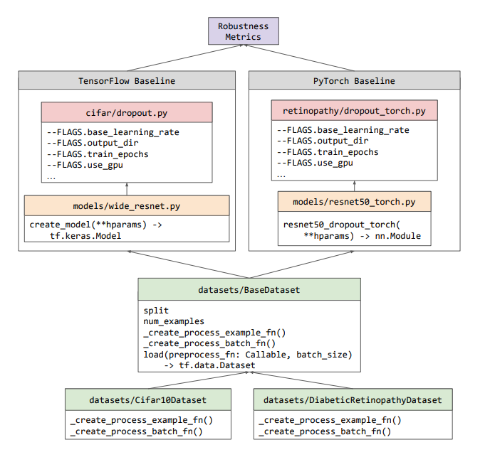
Finally, due to its success for both language and vision tasks, like BERT and ViT, we adopt the Transformer architecture as the backbone of our model, which, unlike prior ROI-based VLP approaches, enables the model to directly take in raw images as inputs. Moreover, inspired by CoAtNet, we adopt a convolution stage consisting of the first three blocks of ResNet in order to extract contextualized patches, which we find more advantageous than the naïve linear projection in the original ViT model. The overall model architecture is illustrated below.

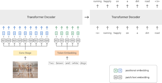
Overview of the SimVLM model architecture.

The model is pre-trained on large-scale web datasets for both image-text and text-only inputs. For joint vision and language data, we use the training set of ALIGN which contains about 1.8B noisy image-text pairs. For text-only data, we use the Colossal Clean Crawled Corpus (C4) dataset introduced by T5, totaling 800G web-crawled documents.

Benchmark Results
After pre-training, we fine-tune our model on the following multimodal tasks: VQA, NLVR2, SNLI-VE, COCO Caption, NoCaps and Multi30K En-De. For example, for VQA the model takes an image and corresponding questions about the input image, and generates the answer as output. We evaluate SimVLM models of three different sizes (base: 86M parameters, large: 307M and huge: 632M) following the same setup as in ViT. We compare our results with strong existing baselines, including LXMERT, VL-T5, UNITER, OSCAR, Villa, SOHO, UNIMO, VinVL, and find that SimVLM achieves state-of-the-art performance across all these tasks despite being much simpler.

VQA       NLVR2       SNLI-VE       CoCo Caption
Model test-dev test-std   dev   test-P dev test B@4 M C S
LXMERT 72.4 72.5 74.9 74.5 - - - - - -
VL-T5 - 70.3 74.6 73.6 - - - - 116.5 -
UNITER 73.8 74 79.1 80 79.4 79.4 - - - -
OSCAR 73.6 73.8 79.1 80.4 - - 41.7 30.6 140 24.5
Villa 74.7 74.9 79.8 81.5 80.2 80 - - - -
SOHO 73.3 73.5 76.4 77.3 85 85 - - - -
UNIMO 75.1 75.3 - - 81.1 80.6 39.6 - 127.7 -
VinVL 76.6 76.6 82.7 84 - - 41 31.1 140.9 25.2
SimVLM base 77.9 78.1 81.7 81.8 84.2 84.2 39 32.9 134.8 24
SimVLM large 79.3 79.6 84.1 84.8 85.7 85.6 40.3 33.4 142.6 24.7
SimVLM huge    80 80.3 84.5 85.2  86.2   86.3   40.6   33.7   143.3   25.4 
Evaluation results on a subset of 6 vision-language benchmarks in comparison with existing baseline models. Metrics used above (higher is better): BLEU-4 (B@4), METEOR (M), CIDEr (C), SPICE (S). Similarly, evaluation on NoCaps and Multi30k En-De also show state-of-the-art performance.

Zero-Shot Generalization
Since SimVLM has been trained on large amounts of data from both visual and textual modalities, it is interesting to ask whether it is capable of performing zero-shot cross-modality transfer. We examine the model on multiple tasks for this purpose, including image captioning, multilingual captioning, open-ended VQA and visual text completion. We take the pre-trained SimVLM and directly decode it for multimodal inputs with fine-tuning only on text data or without fine-tuning entirely. Some examples are given in the figure below. It can be seen that the model is able to generate not only high-quality image captions, but also German descriptions, achieving cross-lingual and cross-modality transfer at the same time.

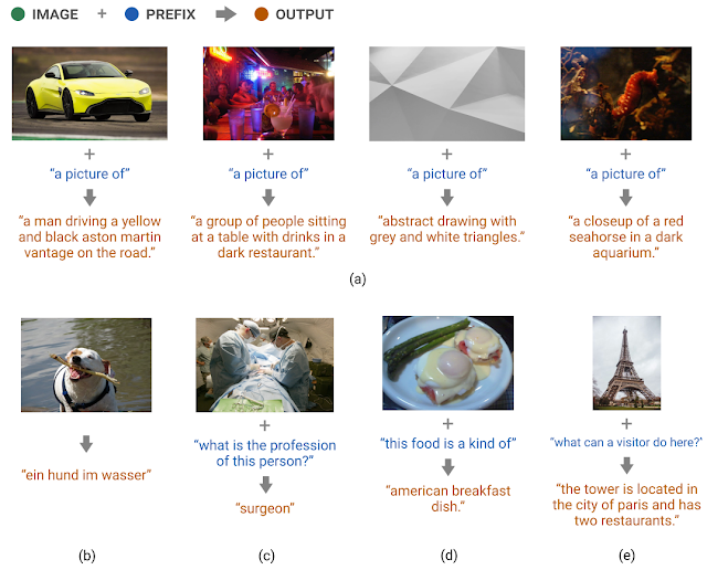
Examples of SimVLM zero-shot generalization. (a) Zero-shot image captioning: Given an image together with text prompts, the pre-trained model predicts the content of the image without fine-tuning. (b) zero-shot cross-modality transfer on German image captioning: The model generates captions in German even though it has never been fine-tuned on image captioning data in German. (c) Generative VQA: The model is capable of generating answers outside the candidates of the original VQA dataset. (d) Zero-shot visual text completion: The pre-trained model completes a textual description grounded on the image contents; (e) Zero-shot open-ended VQA: The model provides factual answers to the questions about images, after continued pre-training on the WIT dataset. Images are from NoCaps, which come from the Open Images dataset under the CC BY 2.0 license.

To quantify SimVLM’s zero-shot performance, we take the pre-trained, frozen model and decode it on the COCO Caption and NoCaps benchmarks, then compare with supervised baselines. Even without supervised fine-tuning (in the middle-rows), SimVLM can reach zero-shot captioning quality close to the quality of supervised methods.

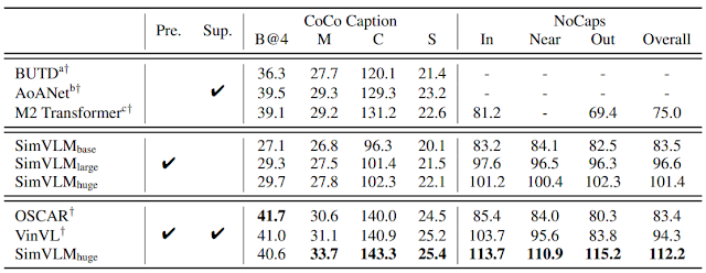
Zero shot image captioning results. Here “Pre.” indicates the model is pre-trained and “Sup.” means the model is finetuned on task-specific supervision. For NoCaps, [In, Near, Out] refer to in-domain, near-domain and out-of-domain respectively. We compare results from BUTD, AoANet, M2 Transformer, OSCAR and VinVL. Metrics used above (higher is better): BLEU-4 (B@4), METEOR (M), CIDEr (C), SPICE (S). For NoCaps, CIDEr numbers are reported.

Conclusion
We propose a simple yet effective framework for VLP. Unlike prior work using object detection models and task-specific auxiliary losses, our model is trained end-to-end with a single prefix language model objective. On various vision-language benchmarks, this approach not only obtains state-of-the-art performance, but also exhibits intriguing zero-shot behaviors in multimodal understanding tasks.

Acknowledgements
We would like to thank Jiahui Yu, Adams Yu, Zihang Dai, Yulia Tsvetkov for preparation of the SimVLM paper, Hieu Pham, Chao Jia, Andrew Dai, Bowen Zhang, Zhifeng Chen, Ruoming Pang, Douglas Eck, Claire Cui and Yonghui Wu for helpful discussions, Krishna Srinivasan, Samira Daruki, Nan Du and Aashi Jain for help with data preparation, Jonathan Shen, Colin Raffel and Sharan Narang for assistance on experimental settings, and others on the Brain team for support throughout this project.

Source: Google AI Blog


Baselines for Uncertainty and Robustness in Deep Learning

Machine learning (ML) is increasingly being used in real-world applications, so understanding the uncertainty and robustness of a model is necessary to ensure performance in practice. For example, how do models behave when deployed on data that differs from the data on which they were trained? How do models signal when they are likely to make a mistake?

To get a handle on an ML model's behavior, its performance is often measured against a baseline for the task of interest. With each baseline, researchers must try to reproduce results only using descriptions from the corresponding papers , which results in serious challenges for replication. Having access to the code for experiments may be more useful, assuming it is well-documented and maintained. But even this is not enough, because the baselines must be rigorously validated. For example, in retrospective analyses over a collection of works [1, 2, 3], authors often find that a simple well-tuned baseline outperforms more sophisticated methods. In order to truly understand how models perform relative to each other, and enable researchers to measure whether new ideas in fact yield meaningful progress, models of interest must be compared to a common baseline.

In “Uncertainty Baselines: Benchmarks for Uncertainty & Robustness in Deep Learning”, we introduce Uncertainty Baselines, a collection of high-quality implementations of standard and state-of-the-art deep learning methods for a variety of tasks, with the goal of making research on uncertainty and robustness more reproducible. The collection spans 19 methods across nine tasks, each with at least five metrics. Each baseline is a self-contained experiment pipeline with easily reusable and extendable components and with minimal dependencies outside of the framework in which it is written. The included pipelines are implemented in TensorFlow, PyTorch, and Jax. Additionally, the hyperparameters for each baseline have been extensively tuned over numerous iterations so as to provide even stronger results.

Uncertainty Baselines
As of this writing, Uncertainty Baselines provides a total of 83 baselines, comprising 19 methods encompassing standard and more recent strategies over nine datasets. Example methods include BatchEnsemble, Deep Ensembles, Rank-1 Bayesian Neural Nets, Monte Carlo Dropout, and Spectral-normalized Neural Gaussian Processes. It acts as a successor in merging several popular benchmarks in the community: Can You Trust Your Model's Uncertainty?, BDL benchmarks, and Edward2's baselines.

Dataset Inputs Output Train Examples Test Datasets
CIFAR RGB images 10-class distribution 50,000 3
ImageNet RGB images 1000-class distribution 1,281,167 6
CLINC Intent Detection Dialog system query text 150-class distribution (in 10 domains) 15,000 2
Kaggle's Diabetic Retinopathy Detection RGB images Probability of Diabetic Retinopathy 35,126 1
Wikipedia Toxicity Wikipedia comment text Probability of toxicity 159,571 3

A subset of 5 out of 9 available datasets for which baselines are provided. The datasets span tabular, text, and image modalities.

Uncertainty Baselines sets up each baseline under a choice of base model, training dataset, and a suite of evaluation metrics. Each is then tuned over its hyperparameters to maximize performance on such metrics. The available baselines vary among these three axes:

Modularity and Reusability
In order for researchers to use and build on the baselines, we deliberately optimized them to be as modular and minimal as possible. As seen in the workflow figure below, Uncertainty Baselines introduces no new class abstractions, instead reusing classes that pre-exist in the ecosystem (e.g., TensorFlow’s tf.data.Dataset). The train/evaluation pipeline for each of the baselines is contained in a standalone Python file for that experiment, which can run on CPU, GPU, or Google Cloud TPUs. Because of this independence between baselines, we are able to develop baselines in any of TensorFlow, PyTorch or JAX.

Workflow diagram for how the different components of Uncertainty Baselines are structured. All datasets are subclasses of the BaseDataset class, which provides a simple API for use in baselines written with any of the supported frameworks. The outputs from any of the baselines can then be analyzed with the Robustness Metrics library.

One area of debate among research engineers is how to manage hyperparameters and other experiment configuration values, which can easily number in the dozens. Instead of using one of the many frameworks built for this, and risk users having to learn yet another library, we opted to simply use Python flags, i.e., flags defined using Abseil that follow Python conventions. This should be a familiar technique to most researchers, and is easy to extend and plug into other pipelines.

Reproducibility
In addition to being able to run each of our baselines using the documented commands and get the same reported results, we also aim to release hyperparameter tuning results and final model checkpoints for further reproducibility. Right now we only have these fully open-sourced for the Diabetic Retinopathy baselines, but we will continue to upload more results as we run them. Additionally, we have examples of baselines that are exactly reproducible up to hardware determinism.

Practical Impact
Each of the baselines included in our repository has gone through extensive hyperparameter tuning, and we hope that researchers can readily reuse this effort without the need for expensive retraining or retuning. Additionally, we hope to avoid minor differences in the pipeline implementations affecting baseline comparisons.

Uncertainty Baselines has already been used in numerous research projects. If you are a researcher with other methods or datasets you would like to contribute, please open a GitHub issue to start a discussion!

Acknowledgements
We would like to thank a number of folks who are codevelopers, provided guidance, and/or helped review this post: Neil Band, Mark Collier, Josip Djolonga, Michael W. Dusenberry, Sebastian Farquhar, Angelos Filos, Marton Havasi, Rodolphe Jenatton, Ghassen Jerfel, Jeremiah Liu, Zelda Mariet, Jeremy Nixon, Shreyas Padhy, Jie Ren, Tim G. J. Rudner, Yeming Wen, Florian Wenzel, Kevin Murphy, D. Sculley, Balaji Lakshminarayanan, Jasper Snoek, Yarin Gal.

Source: Google AI Blog


An ML-Based Framework for COVID-19 Epidemiology

Over the past 20 months, the COVID-19 pandemic has had a profound impact on daily life, presented logistical challenges for businesses planning for supply and demand, and created difficulties for governments and organizations working to support communities with timely public health responses. While there have been well-studied epidemiology models that can help predict COVID-19 cases and deaths to help with these challenges, this pandemic has generated an unprecedented amount of real-time publicly-available data, which makes it possible to use more advanced machine learning techniques in order to improve results.

In "A prospective evaluation of AI-augmented epidemiology to forecast COVID-19 in the USA and Japan", accepted to npj Digital Medicine, we continued our previous work [1, 2, 3, 4] and proposed a framework designed to simulate the effect of certain policy changes on COVID-19 deaths and cases, such as school closings or a state-of-emergency at a US-state, US-county, and Japan-prefecture level, using only publicly-available data. We conducted a 2-month prospective assessment of our public forecasts, during which our US model tied or outperformed all other 33 models on COVID19 Forecast Hub. We also released a fairness analysis of the performance on protected sub-groups in the US and Japan. Like other Google initiatives to help with COVID-19 [1, 2, 3], we are releasing daily forecasts based on this work to the public for free, on the web [us, ja] and through BigQuery.

Prospective forecasts for the USA and Japan models. Ground truth cumulative deaths counts (green lines) are shown alongside the forecasts for each day. Each daily forecast contains a predicted increase in deaths for each day during the prediction window of 4 weeks (shown as colored dots, where shading shifting to yellow indicates days further from the date of prediction in the forecasting horizon, up to 4 weeks). Predictions of deaths are shown for the USA (above) and Japan (below).

The Model
Models for infectious diseases have been studied by epidemiologists for decades. Compartmental models are the most common, as they are simple, interpretable, and can fit different disease phases effectively. In compartmental models, individuals are separated into mutually exclusive groups, or compartments, based on their disease status (such as susceptible, exposed, or recovered), and the rates of change between these compartments are modeled to fit the past data. A population is assigned to compartments representing disease states, with people flowing between states as their disease status changes.

In this work, we propose a few extensions to the Susceptible-Exposed-Infectious-Removed (SEIR) type compartmental model. For example, susceptible people becoming exposed causes the susceptible compartment to decrease and the exposed compartment to increase, with a rate that depends on disease spreading characteristics. Observed data for COVID-19 associated outcomes, such as confirmed cases, hospitalizations and deaths, are used for training of compartmental models.

Visual explanation of "compartmental” models in epidemiology. People "flow" between compartments. Real-world events, like policy changes and more ICU beds, change the rate of flow between compartments.

Our framework proposes a number of novel technical innovations:

  1. Learned transition rates: Instead of using static rates for transitions between compartments across all locations and times, we use machine-learned rates to map them. This allows us to take advantage of the vast amount of available data with informative signals, such as Google's COVID-19 Community Mobility Reports, healthcare supply, demographics, and econometrics features.
  2. Explainability: Our framework provides explainability for decision makers, offering insights on disease propagation trends via its compartmental structure, and suggesting which factors may be most important for driving compartmental transitions.
  3. Expanded compartments: We add hospitalization, ICU, ventilator, and vaccine compartments and demonstrate efficient training despite data sparsity.
  4. Information sharing across locations: As opposed to fitting to an individual location, we have a single model for all locations in a country (e.g., >3000 US counties) with distinct dynamics and characteristics, and we show the benefit of transferring information across locations.
  5. Seq2seq modeling: We use a sequence-to-sequence model with a novel partial teacher forcing approach that minimizes amplified growth of errors into the future.

Forecast Accuracy
Each day, we train models to predict COVID-19 associated outcomes (primarily deaths and cases) 28 days into the future. We report the mean absolute percentage error (MAPE) for both a country-wide score and a location-level score, with both cumulative values and weekly incremental values for COVID-19 associated outcomes.

We compare our framework with alternatives for the US from the COVID19 Forecast Hub. In MAPE, our models outperform all other 33 models except one — the ensemble forecast that also includes our model’s predictions, where the difference is not statistically significant.

We also used prediction uncertainty to estimate whether a forecast is likely to be accurate. If we reject forecasts that the model considers uncertain, we can improve the accuracy of the forecasts that we do release. This is possible because our model has well-calibrated uncertainty.

Mean average percentage error (MAPE, the lower the better) decreases as we remove uncertain forecasts, increasing accuracy.

What-If Tool to Simulate Pandemic Management Policies and Strategies
In addition to understanding the most probable scenario given past data, decision makers are interested in how different decisions could affect future outcomes, for example, understanding the impact of school closures, mobility restrictions and different vaccination strategies. Our framework allows counterfactual analysis by replacing the forecasted values for selected variables with their counterfactual counterparts. The results of our simulations reinforce the risk of prematurely relaxing non-pharmaceutical interventions (NPIs) until the rapid disease spreading is reduced. Similarly, the Japan simulations show that maintaining the State of Emergency while having a high vaccination rate greatly reduces infection rates.

What-if simulations on the percent change of predicted exposed individuals assuming different non-pharmaceutical interventions (NPIs) for the prediction date of March 1, 2021 in Texas, Washington and South Carolina. Increased NPI restrictions are associated with a larger % reduction in the number of exposed people.
What-if simulations on the percent change of predicted exposed individuals assuming different vaccination rates for the prediction date of March 1, 2021 in Texas, Washington and South Carolina. Increased vaccination rate also plays a key role to reduce exposed count in these cases.

Fairness Analysis
To ensure that our models do not create or reinforce unfairly biased decision making, in alignment with our AI Principles, we performed a fairness analysis separately for forecasts in the US and Japan by quantifying whether the model's accuracy was worse on protected sub-groups. These categories include age, gender, income, and ethnicity in the US, and age, gender, income, and country of origin in Japan. In all cases, we demonstrated no consistent pattern of errors among these groups once we controlled for the number of COVID-19 deaths and cases that occur in each subgroup.

Normalized errors by median income. The comparison between the two shows that patterns of errors don't persist once errors are normalized by cases. Left: Normalized errors by median income for the US. Right: Normalized errors by median income for Japan.

Real-World Use Cases
In addition to quantitative analyses to measure the performance of our models, we conducted a structured survey in the US and Japan to understand how organisations were using our model forecasts. In total, seven organisations responded with the following results on the applicability of the model.

  • Organization type: Academia (3), Government (2), Private industry (2)
  • Main user job role: Analyst/Scientist (3), Healthcare professional (1), Statistician (2), Managerial (1)
  • Location: USA (4), Japan (3)
  • Predictions used: Confirmed cases (7), Death (4), Hospitalizations (4), ICU (3), Ventilator (2), Infected (2)
  • Model use case: Resource allocation (2), Business planning (2), scenario planning (1), General understanding of COVID spread (1), Confirm existing forecasts (1)
  • Frequency of use: Daily (1), Weekly (1), Monthly (1)
  • Was the model helpful?: Yes (7)

To share a few examples, in the US, the Harvard Global Health Institute and Brown School of Public Health used the forecasts to help create COVID-19 testing targets that were used by the media to help inform the public. The US Department of Defense used the forecasts to help determine where to allocate resources, and to help take specific events into account. In Japan, the model was used to make business decisions. One large, multi-prefecture company with stores in more than 20 prefectures used the forecasts to better plan their sales forecasting, and to adjust store hours.

Limitations and next steps
Our approach has a few limitations. First, it is limited by available data, and we are only able to release daily forecasts as long as there is reliable, high-quality public data. For instance, public transportation usage could be very useful but that information is not publicly available. Second, there are limitations due to the model capacity of compartmental models as they cannot model very complex dynamics of Covid-19 disease propagation. Third, the distribution of case counts and deaths are very different between the US and Japan. For example, most of Japan's COVID-19 cases and deaths have been concentrated in a few of its 47 prefectures, with the others experiencing low values. This means that our per-prefecture models, which are trained to perform well across all Japanese prefectures, often have to strike a delicate balance between avoiding overfitting to noise while getting supervision from these relatively COVID-19-free prefectures.

We have updated our models to take into account large changes in disease dynamics, such as the increasing number of vaccinations. We are also expanding to new engagements with city governments, hospitals, and private organizations. We hope that our public releases continue to help public and policy-makers address the challenges of the ongoing pandemic, and we hope that our method will be useful to epidemiologists and public health officials in this and future health crises.

Acknowledgements
This paper was the result of hard work from a variety of teams within Google and collaborators around the globe. We'd especially like to thank our paper co-authors from the School of Medicine at Keio University, Graduate School of Public Health at St Luke’s International University, and Graduate School of Medicine at The University of Tokyo.

Source: Google AI Blog


Self-Supervised Learning Advances Medical Image Classification

In recent years, there has been increasing interest in applying deep learning to medical imaging tasks, with exciting progress in various applications like radiology, pathology and dermatology. Despite the interest, it remains challenging to develop medical imaging models, because high-quality labeled data is often scarce due to the time-consuming effort needed to annotate medical images. Given this, transfer learning is a popular paradigm for building medical imaging models. With this approach, a model is first pre-trained using supervised learning on a large labeled dataset (like ImageNet) and then the learned generic representation is fine-tuned on in-domain medical data.

Other more recent approaches that have proven successful in natural image recognition tasks, especially when labeled examples are scarce, use self-supervised contrastive pre-training, followed by supervised fine-tuning (e.g., SimCLR and MoCo). In pre-training with contrastive learning, generic representations are learned by simultaneously maximizing agreement between differently transformed views of the same image and minimizing agreement between transformed views of different images. Despite their successes, these contrastive learning methods have received limited attention in medical image analysis and their efficacy is yet to be explored.

In “Big Self-Supervised Models Advance Medical Image Classification”, to appear at the International Conference on Computer Vision (ICCV 2021), we study the effectiveness of self-supervised contrastive learning as a pre-training strategy within the domain of medical image classification. We also propose Multi-Instance Contrastive Learning (MICLe), a novel approach that generalizes contrastive learning to leverage special characteristics of medical image datasets. We conduct experiments on two distinct medical image classification tasks: dermatology condition classification from digital camera images (27 categories) and multilabel chest X-ray classification (5 categories). We observe that self-supervised learning on ImageNet, followed by additional self-supervised learning on unlabeled domain-specific medical images, significantly improves the accuracy of medical image classifiers. Specifically, we demonstrate that self-supervised pre-training outperforms supervised pre-training, even when the full ImageNet dataset (14M images and 21.8K classes) is used for supervised pre-training.

SimCLR and Multi Instance Contrastive Learning (MICLe)
Our approach consists of three steps: (1) self-supervised pre-training on unlabeled natural images (using SimCLR); (2) further self-supervised pre-training using unlabeled medical data (using either SimCLR or MICLe); followed by (3) task-specific supervised fine-tuning using labeled medical data.

Our approach comprises three steps: (1) Self-supervised pre-training on unlabeled ImageNet using SimCLR (2) Additional self-supervised pre-training using unlabeled medical images. If multiple images of each medical condition are available, a novel Multi-Instance Contrastive Learning (MICLe) strategy is used to construct more informative positive pairs based on different images. (3) Supervised fine-tuning on labeled medical images. Note that unlike step (1), steps (2) and (3) are task and dataset specific.

After the initial pre-training with SimCLR on unlabeled natural images is complete, we train the model to capture the special characteristics of medical image datasets. This, too, can be done with SimCLR, but this method constructs positive pairs only through augmentation and does not readily leverage patients' meta data for positive pair construction. Alternatively, we use MICLe, which uses multiple images of the underlying pathology for each patient case, when available, to construct more informative positive pairs for self-supervised learning. Such multi-instance data is often available in medical imaging datasets — e.g., frontal and lateral views of mammograms, retinal fundus images from each eye, etc.

Given multiple images of a given patient case, MICLe constructs a positive pair for self-supervised contrastive learning by drawing two crops from two distinct images from the same patient case. Such images may be taken from different viewing angles and show different body parts with the same underlying pathology. This presents a great opportunity for self-supervised learning algorithms to learn representations that are robust to changes of viewpoint, imaging conditions, and other confounding factors in a direct way. MICLe does not require class label information and only relies on different images of an underlying pathology, the type of which may be unknown.

MICLe generalizes contrastive learning to leverage special characteristics of medical image datasets (patient metadata) to create realistic augmentations, yielding further performance boost of image classifiers.

Combining these self-supervised learning strategies, we show that even in a highly competitive production setting we can achieve a sizable gain of 6.7% in top-1 accuracy on dermatology skin condition classification and an improvement of 1.1% in mean AUC on chest X-ray classification, outperforming strong supervised baselines pre-trained on ImageNet (the prevailing protocol for training medical image analysis models). In addition, we show that self-supervised models are robust to distribution shift and can learn efficiently with only a small number of labeled medical images.

Comparison of Supervised and Self-Supervised Pre-training
Despite its simplicity, we observe that pre-training with MICLe consistently improves the performance of dermatology classification over the original method of pre-training with SimCLR under different pre-training dataset and base network architecture choices. Using MICLe for pre-training, translates to (1.18 ± 0.09)% increase in top-1 accuracy for dermatology classification over using SimCLR. The results demonstrate the benefit accrued from utilizing additional metadata or domain knowledge to construct more semantically meaningful augmentations for contrastive pre-training. In addition, our results suggest that wider and deeper models yield greater performance gains, with ResNet-152 (2x width) models often outperforming ResNet-50 (1x width) models or smaller counterparts.

Comparison of supervised and self-supervised pre-training, followed by supervised fine-tuning using two architectures on dermatology and chest X-ray classification. Self-supervised learning utilizes unlabeled domain-specific medical images and significantly outperforms supervised ImageNet pre-training.

Improved Generalization with Self-Supervised Models
For each task we perform pretraining and fine-tuning using the in-domain unlabeled and labeled data respectively. We also use another dataset obtained in a different clinical setting as a shifted dataset to further evaluate the robustness of our method to out-of-domain data. For the chest X-ray task, we note that self-supervised pre-training with either ImageNet or CheXpert data improves generalization, but stacking them both yields further gains. As expected, we also note that when only using ImageNet for self-supervised pre-training, the model performs worse compared to using only in-domain data for pre-training.

To test the performance under distribution shift, for each task, we held out additional labeled datasets for testing that were collected under different clinical settings. We find that the performance improvement in the distribution-shifted dataset (ChestX-ray14) by using self-supervised pre-training (both using ImageNet and CheXpert data) is more pronounced than the original improvement on the CheXpert dataset. This is a valuable finding, as generalization under distribution shift is of paramount importance to clinical applications. On the dermatology task, we observe similar trends for a separate shifted dataset that was collected in skin cancer clinics and had a higher prevalence of malignant conditions. This demonstrates that the robustness of the self-supervised representations to distribution shifts is consistent across tasks.

Evaluation of models on distribution-shifted datasets for the chest-xray interpretation task. We use the model trained on in-domain data to make predictions on an additional shifted dataset without any further fine-tuning (zero-shot transfer learning). We observe that self-supervised pre-training leads to better representations that are more robust to distribution shifts.
Evaluation of models on distribution-shifted datasets for the dermatology task. Our results generally suggest that self-supervised pre-trained models can generalize better to distribution shifts with MICLe pre-training leading to the most gains.

Improved Label Efficiency
We further investigate the label-efficiency of the self-supervised models for medical image classification by fine-tuning the models on different fractions of labeled training data. We use label fractions ranging from 10% to 90% for both Derm and CheXpert training datasets and examine how the performance varies using the different available label fractions for the dermatology task. First, we observe that pre-training using self-supervised models can compensate for low label efficiency for medical image classification, and across the sampled label fractions, self-supervised models consistently outperform the supervised baseline. These results also suggest that MICLe yields proportionally higher gains when fine-tuning with fewer labeled examples. In fact, MICLe is able to match baselines using only 20% of the training data for ResNet-50 (4x) and 30% of the training data for ResNet152 (2x).

Top-1 accuracy for dermatology condition classification for MICLe, SimCLR, and supervised models under different unlabeled pre-training datasets and varied sizes of label fractions. MICLe is able to match baselines using only 20% of the training data for ResNet-50 (4x).

Conclusion
Supervised pre-training on natural image datasets is commonly used to improve medical image classification. We investigate an alternative strategy based on self-supervised pre-training on unlabeled natural and medical images and find that it can significantly improve upon supervised pre-training, the standard paradigm for training medical image analysis models. This approach can lead to models that are more accurate and label efficient and are robust to distribution shifts. In addition, our proposed Multi-Instance Contrastive Learning method (MICLe) enables the use of additional metadata to create realistic augmentations, yielding further performance boost of image classifiers.

Self-supervised pre-training is much more scalable than supervised pre-training because class label annotation is not required. We hope this paper will help popularize the use of self-supervised approaches in medical image analysis yielding label efficient and robust models suited for clinical deployment at scale in the real world.

Acknowledgements
This work involved collaborative efforts from a multidisciplinary team of researchers, software engineers, clinicians, and cross-functional contributors across Google Health and Google Brain. We thank our co-authors: Basil Mustafa, Fiona Ryan, Zach Beaver, Jan Freyberg, Jon Deaton, Aaron Loh, Alan Karthikesalingam, Simon Kornblith, Ting Chen, Vivek Natarajan, and Mohammad Norouzi. We also thank Yuan Liu from Google Health for valuable feedback and our partners for access to the datasets used in the research.

Source: Google AI Blog


Google at ICCV 2021

The International Conference on Computer Vision 2021 (ICCV 2021), one of the world's premier conferences on computer vision, starts this week. A Champion Sponsor and leader in computer vision research, Google will have a strong presence at ICCV 2021 with more than 50 research presentations and involvement in the organization of a number of workshops and tutorials.

If you are attending ICCV this year, we hope you’ll check out the work of our researchers who are actively pursuing the latest innovations in computer vision. Learn more about our research being presented in the list below (Google affilitation in bold).

Organizing Committee
Diversity and Inclusion Chair: Negar Rostamzadeh
Area Chairs: Andrea Tagliasacchi, Boqing Gong, Ce Liu, Dilip Krishnan, Jordi Pont-Tuset, Michael Rubinstein, Michael S. Ryoo, Negar Rostamzadeh, Noah Snavely, Rodrigo Benenson, Tsung-Yi Lin, Vittorio Ferrari

Publications
MosaicOS: A Simple and Effective Use of Object-Centric Images for Long-Tailed Object Detection
Cheng Zhang, Tai-Yu Pan, Yandong Li, Hexiang Hu, Dong Xuan, Soravit Changpinyo, Boqing Gong, Wei-Lun Chao

Learning to Resize Images for Computer Vision Tasks
Hossein Talebi, Peyman Milanfar

Joint Representation Learning and Novel Category Discovery on Single- and Multi-Modal Data
Xuhui Jia, Kai Han, Yukun Zhu, Bradley Green

Explaining in Style: Training a GAN to Explain a Classifier in StyleSpace
Oran Lang, Yossi Gandelsman, Michal Yarom, Yoav Wald, Gal Elidan, Avinatan Hassidim, William T. Freeman, Phillip Isola, Amir Globerson, Michal Irani, Inbar Mosseri

Learning Fast Sample Re-weighting without Reward Data
Zizhao Zhang, Tomas Pfister

Contrastive Multimodal Fusion with TupleInfoNCE
Yunze Liu, Qingnan Fan, Shanghang Zhang, Hao Dong, Thomas Funkhouser, Li Yi

Learning Temporal Dynamics from Cycles in Narrated Video
Dave Epstein*, Jiajun Wu, Cordelia Schmid, Chen Sun

Patch Craft: Video Denoising by Deep Modeling and Patch Matching
Gregory Vaksman, Michael Elad, Peyman Milanfar

How to Train Neural Networks for Flare Removal
Yicheng Wu*, Qiurui He, Tianfan Xue, Rahul Garg, Jiawen Chen, Ashok Veeraraghavan, Jonathan T. Barron

Learning to Reduce Defocus Blur by Realistically Modeling Dual-Pixel Data
Abdullah Abuolaim*, Mauricio Delbracio, Damien Kelly, Michael S. Brown, Peyman Milanfar

Hybrid Neural Fusion for Full-Frame Video Stabilization
Yu-Lun Liu, Wei-Sheng Lai, Ming-Hsuan Yang, Yung-Yu Chuang, Jia-Bin Huang

A Dark Flash Normal Camera
Zhihao Xia*, Jason Lawrence, Supreeth Achar

Efficient Large Scale Inlier Voting for Geometric Vision Problems
Dror Aiger, Simon Lynen, Jan Hosang, Bernhard Zeisl

Big Self-Supervised Models Advance Medical Image Classification
Shekoofeh Azizi, Basil Mustafa, Fiona Ryan*, Zachary Beaver, Jan Freyberg, Jonathan Deaton, Aaron Loh, Alan Karthikesalingam, Simon Kornblith, Ting Chen, Vivek Natarajan, Mohammad Norouzi

Physics-Enhanced Machine Learning for Virtual Fluorescence Microscopy
Colin L. Cooke, Fanjie Kong, Amey Chaware, Kevin C. Zhou, Kanghyun Kim, Rong Xu, D. Michael Ando, Samuel J. Yang, Pavan Chandra Konda, Roarke Horstmeyer

Retrieve in Style: Unsupervised Facial Feature Transfer and Retrieval
Min Jin Chong, Wen-Sheng Chu, Abhishek Kumar, David Forsyth

Deep Survival Analysis with Longitudinal X-Rays for COVID-19
Michelle Shu, Richard Strong Bowen, Charles Herrmann, Gengmo Qi, Michele Santacatterina, Ramin Zabih

MUSIQ: Multi-Scale Image Quality Transformer
Junjie Ke, Qifei Wang, Yilin Wang, Peyman Milanfar, Feng Yang

imGHUM: Implicit Generative Models of 3D Human Shape and Articulated Pose
Thiemo Alldieck, Hongyi Xu, Cristian Sminchisescu

Deep Hybrid Self-Prior for Full 3D Mesh Generation
Xingkui Wei, Zhengqing Chen, Yanwei Fu, Zhaopeng Cui, Yinda Zhang

Differentiable Surface Rendering via Non-Differentiable Sampling
Forrester Cole, Kyle Genova, Avneesh Sud, Daniel Vlasic, Zhoutong Zhang

A Lazy Approach to Long-Horizon Gradient-Based Meta-Learning
Muhammad Abdullah Jamal, Liqiang Wang, Boqing Gong

ViViT: A Video Vision Transformer
Anurag Arnab, Mostafa Dehghani, Georg Heigold, Chen Sun, Mario Lučić, Cordelia Schmid

The Surprising Impact of Mask-Head Architecture on Novel Class Segmentation (see the blog post)
Vighnesh Birodkar, Zhichao Lu, Siyang Li, Vivek Rathod, Jonathan Huang

Generalize Then Adapt: Source-Free Domain Adaptive Semantic Segmentation
Jogendra Nath Kundu, Akshay Kulkarni, Amit Singh, Varun Jampani, R. Venkatesh Babu

Unified Graph Structured Models for Video Understanding
Anurag Arnab, Chen Sun, Cordelia Schmid

The Many Faces of Robustness: A Critical Analysis of Out-of-Distribution Generalization
Dan Hendrycks, Steven Basart, Norman Mu, Saurav Kadavath, Frank Wang, Evan Dorundo, Rahul Desai, Tyler Zhu, Samyak Parajuli, Mike Guo, Dawn Song, Jacob Steinhardt, Justin Gilmer

Learning Rare Category Classifiers on a Tight Labeling Budget
Ravi Teja Mullapudi, Fait Poms, William R. Mark, Deva Ramanan, Kayvon Fatahalian

Composable Augmentation Encoding for Video Representation Learning
Chen Sun, Arsha Nagrani, Yonglong Tian, Cordelia Schmid

Multi-Task Self-Training for Learning General Representations
Golnaz Ghiasi, Barret Zoph, Ekin D. Cubuk, Quoc V. Le, Tsung-Yi Lin

With a Little Help From My Friends: Nearest-Neighbor Contrastive Learning of Visual Representations
Debidatta Dwibedi, Yusuf Aytar, Jonathan Tompson, Pierre Sermanet, Andrew Zisserman

Understanding Robustness of Transformers for Image Classification
Srinadh Bhojanapalli, Ayan Chakrabarti, Daniel Glasner, Daliang Li, Thomas Unterthiner, Andreas Veit

Impact of Aliasing on Generalization in Deep Convolutional Networks
Cristina Vasconcelos, Hugo Larochelle, Vincent Dumoulin, Rob Romijnders, Nicolas Le Roux, Ross Goroshin

von Mises-Fisher Loss: An Exploration of Embedding Geometries for Supervised Learning
Tyler R. Scott*, Andrew C. Gallagher, Michael C. Mozer

Contrastive Learning for Label Efficient Semantic Segmentation
Xiangyun Zhao*, Raviteja Vemulapalli, Philip Andrew Mansfield, Boqing Gong, Bradley Green, Lior Shapira, Ying Wu

Interacting Two-Hand 3D Pose and Shape Reconstruction from Single Color Image
Baowen Zhang, Yangang Wang, Xiaoming Deng, Yinda Zhang, Ping Tan, Cuixia Ma, Hongan Wang

Telling the What While Pointing to the Where: Multimodal Queries for Image Retrieval
Soravit Changpinyo, Jordi Pont-Tuset, Vittorio Ferrari, Radu Soricut

SO-Pose: Exploiting Self-Occlusion for Direct 6D Pose Estimation
Yan Di, Fabian Manhardt, Gu Wang, Xiangyang Ji, Nassir Navab, Federico Tombari

Patch2CAD: Patchwise Embedding Learning for In-the-Wild Shape Retrieval from a Single Image
Weicheng Kuo, Anelia Angelova, Tsung-Yi Lin, Angela Dai

NeRD: Neural Reflectance Decomposition From Image Collections
Mark Boss, Raphael Braun, Varun Jampani, Jonathan T. Barron, Ce Liu, Hendrik P.A. Lensch

THUNDR: Transformer-Based 3D Human Reconstruction with Markers
Mihai Zanfir, Andrei Zanfir, Eduard Gabriel Bazavan, William T. Freeman, Rahul Sukthankar, Cristian Sminchisescu

Discovering 3D Parts from Image Collections
Chun-Han Yao, Wei-Chih Hung, Varun Jampani, Ming-Hsuan Yang

Multiresolution Deep Implicit Functions for 3D Shape Representation
Zhang Chen*, Yinda Zhang, Kyle Genova, Sean Fanello, Sofien Bouaziz, Christian Hane, Ruofei Du, Cem Keskin, Thomas Funkhouser, Danhang Tang

AI Choreographer: Music Conditioned 3D Dance Generation With AIST++ (see the blog post)
Ruilong Li*, Shan Yang, David A. Ross, Angjoo Kanazawa

Learning Object-Compositional Neural Radiance Field for Editable Scene Rendering
Bangbang Yang, Han Zhou, Yinda Zhang, Hujun Bao, Yinghao Xu, Guofeng Zhang, Yijin Li, Zhaopeng Cui

VariTex: Variational Neural Face Textures
Marcel C. Buhler, Abhimitra Meka, Gengyan Li, Thabo Beeler, Otmar Hilliges

Pathdreamer: A World Model for Indoor Navigation (see the blog post)
Jing Yu Koh, Honglak Lee, Yinfei Yang, Jason Baldridge, Peter Anderson

4D-Net for Learned Multi-Modal Alignment
AJ Piergiovanni, Vincent Casser, Michael S. Ryoo, Anelia Angelova

Episodic Transformer for Vision-and-Language Navigation
Alexander Pashevich*, Cordelia Schmid, Chen Sun

Graph-to-3D: End-to-End Generation and Manipulation of 3D Scenes Using Scene Graphs
Helisa Dhamo, Fabian Manhardt, Nassir Navab, Federico Tombari

Unconditional Scene Graph Generation
Sarthak Garg, Helisa Dhamo, Azade Farshad, Sabrina Musatian, Nassir Navab, Federico Tombari

Panoptic Narrative Grounding
Cristina González, Nicolás Ayobi, Isabela Hernández, José Hernández, Jordi Pont-Tuset, Pablo Arbeláez

Cross-Camera Convolutional Color Constancy
Mahmoud Afifi*, Jonathan T. Barron, Chloe LeGendre, Yun-Ta Tsai, Francois Bleibel

Defocus Map Estimation and Deblurring from a Single Dual-Pixel Image
Shumian Xin*, Neal Wadhwa, Tianfan Xue, Jonathan T. Barron, Pratul P. Srinivasan, Jiawen Chen, Ioannis Gkioulekas, Rahul Garg

COMISR: Compression-Informed Video Super-Resolution
Yinxiao Li, Pengchong Jin, Feng Yang, Ce Liu, Ming-Hsuan Yang, Peyman Milanfar

Mip-NeRF: A Multiscale Representation for Anti-Aliasing Neural Radiance Fields
Jonathan T. Barron, Ben Mildenhall, Matthew Tancik, Peter Hedman, Ricardo Martin-Brualla, Pratul P. Srinivasan

Nerfies: Deformable Neural Radiance Fields
Keunhong Park*, Utkarsh Sinha, Jonathan T. Barron, Sofien Bouaziz, Dan B Goldman, Steven M. Seitz, Ricardo Martin-Brualla

Baking Neural Radiance Fields for Real-Time View Synthesis
Peter Hedman, Pratul P. Srinivasan, Ben Mildenhall, Jonathan T. Barron, Paul Debevec

Stacked Homography Transformations for Multi-View Pedestrian Detection
Liangchen Song, Jialian Wu, Ming Yang, Qian Zhang, Yuan Li, Junsong Yuan

COTR: Correspondence Transformer for Matching Across Images
Wei Jiang, Eduard Trulls, Jan Hosang, Andrea Tagliasacchi, Kwang Moo Yi

Large Scale Interactive Motion Forecasting for Autonomous Driving: The Waymo Open Motion Dataset
Scott Ettinger, Shuyang Cheng, Benjamin Caine, Chenxi Liu, Hang Zhao, Sabeek Pradhan, Yuning Chai, Ben Sapp, Charles R. Qi, Yin Zhou, Zoey Yang, Aurélien Chouard, Pei Sun, Jiquan Ngiam, Vijay Vasudevan, Alexander McCauley, Jonathon Shlens, Dragomir Anguelov

Low-Shot Validation: Active Importance Sampling for Estimating Classifier Performance on Rare Categories
Fait Poms, Vishnu Sarukkai, Ravi Teja Mullapudi, Nimit S. Sohoni, William R. Mark, Deva Ramanan, Kayvon Fatahalian

Vector Neurons: A General Framework for SO(3)-Equivariant Networks
Congyue Deng, Or Litany, Yueqi Duan, Adrien Poulenard, Andrea Tagliasacchi, Leonidas J. Guibas

SLIDE: Single Image 3D Photography with Soft Layering and Depth-Aware Inpainting
Varun Jampani, Huiwen Chang, Kyle Sargent, Abhishek Kar, Richard Tucker, Michael Krainin, Dominik Kaeser, William T. Freeman, David Salesin, Brian Curless, Ce Liu

DeepPanoContext: Panoramic 3D Scene Understanding with Holistic Scene Context Graph and Relation-Based Optimization
Cheng Zhang, Zhaopeng Cui, Cai Chen, Shuaicheng Liu, Bing Zeng, Hujun Bao, Yinda Zhang

Infinite Nature: Perpetual View Generation of Natural Scenes from a Single Image
Andrew Liu, Richard Tucker, Varun Jampani, Ameesh Makadia, Noah Snavely, Angjoo Kanazawa

Workshops (only Google affiliations are noted)
Visual Inductive Priors for Data-Efficient Deep Learning Workshop
Speakers: Ekin Dogus Cubuk, Chelsea Finn

Instance-Level Recognition Workshop
Organizers: Andre Araujo, Cam Askew, Bingyi Cao, Jack Sim, Tobias Weyand

Unsup3D: Unsupervised 3D Learning in the Wild
Speakers: Adel Ahmadyan, Noah Snavely, Tali Dekel

Embedded and Real-World Computer Vision in Autonomous Driving (ERCVAD 2021)
Speakers: Mingxing Tan

Adversarial Robustness in the Real World
Speakers: Nicholas Carlini

Neural Architectures: Past, Present and Future
Speakers: Been Kim, Hanxiao Liu Organizers: Azade Nazi, Mingxing Tan, Quoc V. Le

Computational Challenges in Digital Pathology
Organizers: Craig Mermel, Po-Hsuan Cameron Chen

Interactive Labeling and Data Augmentation for Vision
Speakers: Vittorio Ferrari

Map-Based Localization for Autonomous Driving
Speakers: Simon Lynen

DeeperAction: Challenge and Workshop on Localized and Detailed Understanding of Human Actions in Videos
Speakers: Chen Sun Advisors: Rahul Sukthankar

Differentiable 3D Vision and Graphics
Speakers: Angjoo Kanazawa

Deep Multi-Task Learning in Computer Vision
Speakers: Chelsea Finn

Computer Vision for AR/VR
Speakers: Matthias Grundmann, Ira Kemelmacher-Shlizerman

GigaVision: When Gigapixel Videography Meets Computer Vision
Organizers: Feng Yang

Human Interaction for Robotic Navigation
Speakers: Peter Anderson

Advances in Image Manipulation Workshop and Challenges
Organizers: Ming-Hsuan Yang

More Exploration, Less Exploitation (MELEX)
Speakers: Angjoo Kanazawa

Structural and Compositional Learning on 3D Data
Speakers: Thomas Funkhouser, Kyle Genova Organizers: Fei Xia

Simulation Technology for Embodied AI
Organizers: Li Yi

Video Scene Parsing in the Wild Challenge Workshop
Speakers: Liang-Chieh (Jay) Chen

Structured Representations for Video Understanding
Organizers: Cordelia Schmid

Closing the Loop Between Vision and Language
Speakers: Cordelia Schmid

Segmenting and Tracking Every Point and Pixel: 6th Workshop on Benchmarking Multi-Target Tracking
Organizers: Jun Xie, Liang-Chieh Chen

AI for Creative Video Editing and Understanding
Speakers: Angjoo Kanazawa, Irfan Essa

BEHAVIOR: Benchmark for Everyday Household Activities in Virtual, Interactive, and Ecological Environments
Speakers: Chelsea Finn Organizers: Fei Xia

Computer Vision for Automated Medical Diagnosis
Organizers: Maithra Raghu

Computer Vision for the Factory Floor
Speakers: Cordelia Schmid

Tutorials (only Google affiliations are noted)
Towards Robust, Trustworthy, and Explainable Computer Vision
Speakers: Sara Hooker

Multi-Modality Learning from Videos and Beyond
Organizers: Arsha Nagrani

Tutorial on Large Scale Holistic Video Understanding
Organizers: David Ross

Efficient Video Understanding: State of the Art, Challenges, and Opportunities
Organizers: Arsha Nagrani

* Indicates work done while at Google

Source: Google AI Blog


Finding Complex Metal Oxides for Technology Advancement

A crystalline material has atoms systematically arranged in repeating units, with this structure and the elements it contains determining the material’s properties. For example, silicon’s crystal structure allows it to be widely used in the semiconductor industry, whereas graphite’s soft, layered structure makes for great pencils. One class of crystalline materials that are critical for a wide range of applications, ranging from battery technology to electrolysis of water (i.e., splitting H2O into its component hydrogen and oxygen), are crystalline metal oxides, which have repeating units of oxygen and metals. Researchers suspect that there is a significant number of crystalline metal oxides that could prove to be useful, but their number and the extent of their useful properties is unknown.

In “Discovery of complex oxides via automated experiments and data science”, a collaborative effort with partners at the Joint Center for Artificial Photosynthesis (JCAP), a Department of Energy (DOE) Energy Innovation Hub at Caltech, we present a systematic search for new complex crystalline metal oxides using a novel approach for rapid materials synthesis and characterization. Using a customized inkjet printer to print samples with different ratios of metals, we were able to generate more than 350k distinct compositions, a number of which we discovered had interesting properties. One example, based on cobalt, tantalum and tin, exhibited tunable transparency, catalytic activity, and stability in strong acid electrolytes, a rare combination of properties of importance for renewable energy technologies. To stimulate continued research in this field, we are releasing a database consisting of nine channels of optical absorption measurements, which can be used as an indicator of interesting properties, across 376,752 distinct compositions of 108 3-metal oxide systems, along with model results that identify the most promising compositions for a variety of technical applications.

Background
There are on the order of 100 properties of interest in materials science that are relevant to enhancing existing technologies and to creating new ones, ranging from electrical, optical, and magnetic to thermal and mechanical. Traditionally, exploring materials for a target technology involves considering only one or a few such properties at a time, resulting in many parallel efforts where the same materials are being evaluated. Machine learning (ML) for material properties prediction has been successfully deployed in many of these parallel efforts, but the models are inherently specialized and fail to capture the universality of the prediction problem. Instead of asking traditional questions of how ML can help find a suitable material for a particular property, we instead apply ML to find a short-list of materials that may be exceptional for any given property. This strategy combines high throughput materials experiments with a physics-aware data science workflow.

A challenge in realizing this strategy is that the search space for new crystalline metal oxides is enormous. For example, the Inorganic Crystal Structure Database (ICSD) lists 73 metals that exist in oxides composed of a single metal and oxygen. Generating novel compounds simply by making various combinations of these metals would yield 62,196 possible 3-metal oxide systems, some of which will contain several unique structures. If, in addition, one were to vary the relative quantities of each metal, the set of possible combinations would be orders of magnitude larger.

However, while this search space is large, only a small fraction of these novel compositions will form new crystalline structures, with the majority simply resulting in combinations of existing structures. While these combinations of structures may be interesting for some applications, the goal is to find the core single-structure compositions. Of the possible 3-metal oxide systems, the ICSD reports only 2,205 with experimentally confirmed compositions, indicating that the vast majority of possible compositions either have not been explored or have yielded negative results and have not been published. In the present work we do not directly measure the crystal structures of new materials, but instead use high throughput experiments to enable ML-based inferences of where new structures can be found.

Synthesis
Our goal was to explore a large swath of chemical space as quickly as possible. Whereas traditional synthesis techniques like physical vapor deposition can create high quality thin films, we decided to reuse an existing technology that was already optimized to mix and deposit small amounts of material very quickly: an inkjet printer. We made each metal element printable by dissolving a metal nitrate or metal chloride into an ink solution. We then printed a series of lines on glass plates, where the ratios of the elements used in the printing varied along each line according to our experiment design so that we could generate thousands of unique compositions per plate. Several such plates were then dried and baked together in a series of ovens to oxidize the metals. Due to the inherent variability in the printing, drying, and baking of the plates, we opted to print 10 duplicates of each composition. Even with this level of replication, we still were able to generate novel compositions 100x faster than traditional vapor deposition techniques.

The modified professional grade inkjet printer.
Top: A printed and baked plate that is 10 x 15 cm. Bottom: A close-up of a portion of the plate. Since the optical properties vary with composition, the gradient in composition appears as a color gradient along each line.

Characterization
When making samples at this rate, it is hard to find a characterization technique that can keep up. A traditional approach to design a material for a specific purpose would require significant time to measure the pertinent properties of each combination, but for the analysis to keep up with our high-throughput printing method, we needed something faster. So, we built a custom microscope capable of taking pictures at nine discrete wavelengths ranging from the ultraviolet (385 nm), through the visible, to the infrared (850 nm). This microscope produced over 20 TB of image data over the course of the project, which we used to calculate the optical absorption coefficients of each sample at each wavelength. While optical absorption itself is important for technologies such as solar energy harvesting, in our work we are interested in optical absorption vs. wavelength as a fingerprint of each material.

Analysis
After generating 376,752 distinct compositions, we needed to know which ones were actually interesting. We hypothesized that since the structure of a material determines its properties, when a material property (in this case, the optical absorption spectrum) changes in a nontrivial way, that could indicate a structural change. To test this, we built two ML models to identify potentially interesting compositions.

As the composition of metals changes in a metal oxide, the crystal structure of the resulting material may change. The map of the compositions that crystallize into the same structure, which we call the phase, is the “phase diagram”. The first model, the ‘phase diagram’ model, is a physics-based model that assumes thermodynamic equilibrium, which imposes limits on the number of phases that can coexist. Assuming that the optical properties of a combination of crystalline phases vary linearly with the ratio of each crystalline phase, the model generates a set of phases that best fit the optical absorption spectra. The phase diagram model involved a comprehensive search through the space of thermodynamically allowed phase diagrams. The second model seeks to identify “emergent properties” by identifying 3-metal oxide absorption spectra that can not be explained by a linear combination of 1-metal or 2-metal oxide signals.

Phase analysis of compounds with different relative fractions of the metals iron (Fe), tin (Sn) and yttrium (Y). Left: Panels showing the absorption coefficient at different wavelengths: a) 375 nm; b) 530 nm; c) 660 nm, d) 850 nm. Right: Based on the absorption, the phase diagram model identifies the boundaries at which changes in the relative composition in the compound lead to different optical properties and hence suggest compositions with potentially interesting behavior. In panels e), f) and g), red points are candidate phases, and vertices where blue lines meet indicate interesting phase behavior. Panel h) shows the emergent property model, where compositions are colored by the log-likelihood of their properties being explainable by lower-order compositions (darker colors are more likely to represent more interesting compounds).

Experimental Verification
In the end our systematic, combinatorial sweep of 108 3-metal oxide systems found 51 of these systems exhibited interesting behavior. Of these 108 systems, only 1 of them has an experimentally reported entry in the ICSD. We performed an in-depth experimental study of one unexplored system, the Co-Ta-Sn oxides. With guidance from the high throughput workflow, we validated the discovery of a new family of solid solutions by x-ray diffraction, successfully resynthesized the new materials using a common technique (physical vapor deposition), validated the surprisingly high transparency in compositions with up to 30% Co, and performed follow-up electrochemical testing that demonstrated electrocatalytic activity for water oxidation (a critical step in hydrogen fuel synthesis from water). Catalyst testing for water oxidation is far more expensive than the optical screening from our high throughput workflow, and even though there is no known connection between the optical properties and the catalytic properties, we use the analysis of optical properties to select a small number of compositions for catalyst testing, demonstrating our high level concept of using one high throughput workflow to down-select materials for practically any target technology.

Conclusions
The Co-Ta-Sn oxide example illustrates how finding new materials quickly is an important step in developing improved technologies, such as those critical for hydrogen production. We hope this work inspires the materials community — for the experimentalists, we hope to inspire creativity in aggressively scaling high-throughput techniques, and for computationalists, we hope to provide a rich dataset with plenty of negative results to better inform ML and other data science models.

Acknowledgements
It was a pleasure and a privilege to work with John Gregoire and Joel Haber at Caltech for this complex, long-running project. Additionally, we would like to thank Zan Armstrong, Sam Yang, Kevin Kan, Lan Zhou, Matthias Richter, Chris Roat, Nick Wagner, Marc Coram, Marc Berndl, Pat Riley, and Ted Baltz for their contributions.

Source: Google AI Blog


Introducing FLAN: More generalizable Language Models with Instruction Fine-Tuning

For a machine learning model to generate meaningful text, it must have a large amount of knowledge about the world as well as the ability to abstract. While language models that are trained to do this are increasingly able to automatically acquire this knowledge as they scale, how to best unlock this knowledge and apply it to specific real-world tasks is not clear.

One well-established technique for doing this is called fine-tuning, which is training a pretrained model such as BERT and T5 on a labeled dataset to adapt it to a downstream task. However, fine-tuning requires a large number of training examples, along with stored model weights for each downstream task, which is not always practical, particularly for large models.

In “Fine-tuned Language Models Are Zero-Shot Learners”, we explore a simple technique called instruction fine-tuning, or instruction tuning for short. This involves fine-tuning a model not to solve a specific task, but to make it more amenable to solving NLP tasks in general. We use instruction tuning to train a model, which we call Fine-tuned LAnguage Net (FLAN). Because the instruction tuning phase of FLAN only takes a small number of updates compared to the large amount of computation involved in pre-training the model, it's the metaphorical dessert to the main course of pretraining. This enables FLAN to perform various unseen tasks.

An illustration of how FLAN works: The model is fine-tuned on disparate sets of instructions and generalizes to unseen instructions. As more types of tasks are added to the fine-tuning data model performance improves.

Background
One recent popular technique for using language models to solve tasks is called zero-shot or few-shot prompting. This technique formulates a task based on text that a language model might have seen during training, where then the language model generates the answer by completing the text. For instance, to classify the sentiment of a movie review, a language model might be given the sentence, “The movie review ‘best RomCom since Pretty Woman’ is _” and be asked to complete the sentence with either the word “positive” or “negative”.

Although this technique demonstrates good performance for some tasks, it requires careful prompt engineering to design tasks to look like data that the model has seen during training — an approach that performs well on some but not all tasks and also can be an unintuitive way for practitioners to interact with the model. For example, the creators of GPT-3 (one of the largest language models in use today) found that such prompting techniques did not result in good performance on natural language inference (NLI) tasks

Instruction Tuning
FLAN instead fine-tunes the model on a large set of varied instructions that use a simple and intuitive description of the task, such as “Classify this movie review as positive or negative,” or “Translate this sentence to Danish.”

Creating a dataset of instructions from scratch to fine-tune the model would take a considerable amount of resources. Therefore, we instead make use of templates to transform existing datasets into an instructional format.

Example templates for a natural language inference dataset.

We show that by training a model on these instructions it not only becomes good at solving the kinds of instructions it has seen during training but becomes good at following instructions in general.

Evaluating the Model
To compare FLAN against other techniques in a meaningful way, we used established benchmark datasets to compare the performance of our model with existing models. Also, we evaluated how FLAN performs without having seen any examples from that dataset during training.

However, if we trained on datasets that were too similar to an evaluation dataset, that might still skew the performance results. For example, training on one question-answering dataset might help the model do better on another question-answering dataset. Because of this, we group all datasets into clusters by type of task and hold out not just the training data for the dataset, but the entire task cluster to which the dataset belongs.

We grouped our datasets into the clusters below.

Results
We evaluated FLAN on 25 tasks and found that it improves over zero-shot prompting on all but four of them. We found that our results are better than zero-shot GPT-3 on 20 of 25 tasks, and better than even few-shot GPT-3 on some tasks.

For various models, we show the average accuracy over all datasets in a task cluster. Natural language inference datasets: ANLI R1–R3, CB, and RTE. Reading comprehension datasets: BoolQ, MultiRC, OpenbookQA. Closed-book QA datasets: ARC, NQ, TriviaQA.

We also find that model scale is very important for the ability of the model to benefit from instruction tuning. At smaller scales, the FLAN technique actually degrades performance, and only at larger scales does the model become able to generalize from instructions in the training data to unseen tasks. This might be because models that are too small do not have enough parameters to perform a large number of tasks.

Instruction tuning only improves performance on unseen tasks for models of certain size.

Conclusion
The FLAN model is not the first to train on a set of instructions, but to our knowledge we are the first to apply this technique at scale and show that it can improve the generalization ability of the model. We hope that the method we presented will help inspire more research into models that can perform unseen tasks and learn from very little data.

We also released the code to perform the transformations so that other researchers can reproduce our results and build on them.

Acknowledgements
We thank our collaborators Vincent Y. Zhao, Kelvin Guu, Adams Wei Yu, Brian Lester, Nan Du, Andrew M. Dai, and Quoc V. Le at Google Research.

Source: Google AI Blog


FedJAX: Federated Learning Simulation with JAX

Federated learning is a machine learning setting where many clients (i.e., mobile devices or whole organizations, depending on the task at hand) collaboratively train a model under the orchestration of a central server, while keeping the training data decentralized. For example, federated learning makes it possible to train virtual keyboard language models based on user data that never leaves a mobile device.

Federated learning algorithms accomplish this by first initializing the model at the server and completing three key steps for each round of training:

  1. The server sends the model to a set of sampled clients.
  2. These sampled clients train the model on local data.
  3. After training, the clients send the updated models to the server and the server aggregates them together.
An example federated learning algorithm with four clients.

Federated learning has become a particularly active area of research due to an increased focus on privacy and security. Being able to easily translate ideas into code, iterate quickly, and compare and reproduce existing baselines is important for such a fast growing field.

In light of this, we are excited to introduce FedJAX, a JAX-based open source library for federated learning simulations that emphasizes ease-of-use in research. With its simple building blocks for implementing federated algorithms, prepackaged datasets, models and algorithms, and fast simulation speed, FedJAX aims to make developing and evaluating federated algorithms faster and easier for researchers. In this post we discuss the library structure and contents of FedJAX. We demonstrate that on TPUs FedJAX can be used to train models with federated averaging on the EMNIST dataset in a few minutes, and the Stack Overflow dataset in roughly an hour with standard hyperparameters.

Library Structure
Keeping ease of use in mind, FedJAX introduces only a few new concepts. Code written with FedJAX resembles the pseudo-code used to describe novel algorithms in academic papers, making it easy to get started. Additionally, while FedJAX provides building blocks for federated learning, users can replace these with the most basic implementations using just NumPy and JAX while still keeping the overall training reasonably fast.

Included Dataset and Models
In the current landscape of federated learning research, there are a variety of commonly used datasets and models, such as image recognition, language modeling, and more. A growing number of these datasets and models can be used straight out of the box in FedJAX, so the preprocessed datasets and models do not have to be written from scratch. This not only encourages valid comparisons between different federated algorithms but also accelerates the development of new algorithms.

At present, FedJAX comes packaged with the following datasets and sample models:

In addition to these standard setups, FedJAX provides tools to create new datasets and models that can be used with the rest of the library. Finally, FedJAX comes with standard implementations of federated averaging and other federated algorithms for training a shared model on decentralized examples, such as adaptive federated optimizers, agnostic federated averaging, and Mime, to make comparing and evaluating against existing algorithms easier.

Performance Evaluation
We benchmarked a standard FedJAX implementation of adaptive federated averaging on two tasks: the image recognition task for the federated EMNIST-62 dataset and the next word prediction task for the Stack Overflow dataset. Federated EMNIST-62 is a smaller dataset that consists of 3400 users and their writing samples, which are one of 62 characters (alphanumeric), while the Stack Overflow dataset is much larger and consists of millions of questions and answers from the Stack Overflow forum for hundreds of thousands of users.

We measured performance on various hardware specialized for machine learning. For federated EMNIST-62, we trained a model for 1500 rounds with 10 clients per round on GPU (NVIDIA V100) and TPU (1 TensorCore on a Google TPU v2) accelerators.

For Stack Overflow, we trained a model for 1500 rounds with 50 clients per round on GPU (NVIDIA V100) using jax.jit, TPU (1 TensorCore on a Google TPU v2) using only jax.jit, and multi-core TPU (8 TensorCores on a Google TPU v2) using jax.pmap. In the charts below, we’ve recorded the average training round completion time, time taken for full evaluation on test data, and time for the overall execution, which includes both training and full evaluation.

Benchmark results for federated EMNIST-62.
Benchmark results for Stack Overflow.

With standard hyperparameters and TPUs, the full experiments for federated EMNIST-62 can be completed in a few minutes and roughly an hour for Stack Overflow.

Stack Overflow average training round duration as the number of clients per round increases.

We also evaluate the Stack Overflow average training round duration as the number of clients per round increases. By comparing the average training round duration between TPU (8 cores) and TPU (1 core) in the figure, it is evident that using multiple TPU cores results in considerable runtime improvement if the number of clients participating per round is large (useful for applications like differentially private learning).

Conclusions and Future Work
In this post, we introduced FedJAX, a fast and easy-to-use federated learning simulation library for research. We hope that FedJAX will foster even more investigation and interest in federated learning. Moving forward, we plan to continually grow our existing collection of algorithms, aggregation mechanisms, datasets, and models.

Feel free to take a look at some of our tutorial notebooks, or try out FedJAX yourself! For more information about the library and relationship to platforms, such as Tensorflow Federated, see our paper, README, or FAQs.

Acknowledgements
We would like to thank Ke Wu and Sai Praneeth Kamireddy for contributing to the library and various discussions during development.

We would also like to thank Ehsan Amid, Theresa Breiner, Mingqing Chen, Fabio Costa, Roy Frostig, Zachary Garrett, Alex Ingerman, Satyen Kale, Rajiv Mathews, Lara Mcconnaughey, Brendan McMahan, Mehryar Mohri, Krzysztof Ostrowski, Max Rabinovich, Michael Riley, Vlad Schogol, Jane Shapiro, Gary Sivek, Luciana Toledo-Lopez, and Michael Wunder for helpful comments and contributions.

Source: Google AI Blog


Efficient Partitioning of Road Networks

Design techniques based on classical algorithms have proved useful for recent innovation on several large-scale problems, such as travel itineraries and routing challenges. For example, Dijkstra’s algorithm is often used to compute routes in graphs, but the size of the computation can increase quickly beyond the scale of a small town. The process of "partitioning" a road network, however, can greatly speed up algorithms by effectively shrinking how much of the graph is searched during computation.

In this post, we cover how we engineered a graph partitioning algorithm for road networks using ideas from classic algorithms, parts of which were presented in “Sketch-based Algorithms for Approximate Shortest Paths in Road Networks” at WWW 2021. Using random walks, a classical concept that is counterintuitively useful for computing shortest routes by decreasing the network size significantly, our algorithm can find a high quality partitioning of the whole road network of the North America continent nearly an order of magnitude faster1 than other partitioning algorithms with similar output qualities.

Using Graphs to Model Road Networks
There is a well-known and useful correspondence between road networks and graphs, where intersections become nodes and roads become edges.

Image from Wikipedia

To understand how routing might benefit from partitioning, consider the most well-known solution for finding the fastest route: the Dijkstra algorithm, which works in a breadth-first search manner. The Dijkstra algorithm performs an exhaustive search starting from the source until it finds the destination. Because of this, as the distance between the source and the destination increases, the computation can become an order of magnitude slower. For example, it is faster to compute a route inside Seattle, WA than from Seattle, WA to San Francisco, CA. Moreover, even for intra-metro routes, the exhaustive volume of space explored by the Dijkstra algorithm during computation results in an impractical latency on the order of seconds. However, identifying regions that have more connections inside themselves, but fewer connections to the outside (such as Staten Island, NY) makes it possible to split the computation into multiple, smaller chunks.

Top: A routing problem around Staten Island, NY. Bottom: Corresponding partitioning as a graph. Blue nodes indicate the only entrances to/exits from Staten Island.

Consider driving from point A to point B in the above image. Once one decides where to enter Staten Island (Outerbridge or Goethals) and where to exit (Verrazzano), the problem can be broken into the three smaller pieces of driving: To the entrance, the exit, and then the destination using the best route available. That means a routing algorithm only needs to consider these special points (beacons) to navigate between points A and B and can thus find the shortest accurate path faster.

Note that beacons are only useful as long as there are not too many of them—the fewer beacons there are, the fewer shortcuts need to be added, the smaller the search space, and the faster the computation—so a good partitioning should have relatively fewer beacons for the number of components (i.e., a particular area of a road network).

As the example of Staten Island illustrates, real-life road networks have many beacons (special points such as bridges, tunnels, or mountain passes) that result in some areas being very well-connected (e.g., with large grids of streets) and others being poorly connected (e.g., an island only accessible via a couple of bridges). The question becomes how to efficiently define the components and identify the smallest number of beacons that connect the road network.

Our Partitioning Algorithm
Because each connection between two components is a potential beacon, the approach we take to ensure there are not too many beacons is to divide the road network in a way that minimizes the number of connections between components.

To do this, we start by dividing the network into two balanced (i.e., of similar size) components while also minimizing the number of roads that connect those two components, which results in an effectively small ratio of beacons to roads in each component. Then, the algorithm keeps dividing the network into two at a time until all the components reach the desired size, in terms of the number of roads inside, that yields a useful multi-component partition. There is a careful balance here: If the size is too small, we will get too many beacons; whereas if it is too large, then it will be useful only for long routes. Therefore the size is left as an input parameter and found through experimentation when the algorithm is being finalized.

While there are numerous partitioning schemes, such as METIS (for general networks), PUNCH and inertial-flow (both optimized for road-network likes), our solution is based on the inertial-flow algorithm, augmented to run as efficiently on whole continents as it does on cities.

Balanced Partitioning for Road Networks
How does one divide a road network represented as a graph into two balanced components, as mentioned above? A first step is to make a graph smaller by grouping closely connected nodes together, which allows us to speed up the following two-way partitioning phase. This is where a random walk is useful.

Random walks enjoy many useful theoretical properties—which is why they have been used to study a range of topics from the motion of mosquitoes in a forest to heat diffusion—and that most relevant for our application is that they tend to get “trapped” in regions that are well connected inside but poorly connected outside. Consider a random walk on the streets of Staten Island for a fixed number of steps: because relatively few roads exit the island, most of the steps happen inside the island, and the probability of stepping outside the island is low.

Illustration of a random walk. Suppose the blue graph is a hypothetical road network corresponding to Staten Island. 50 random walks are performed, all starting at the middle point. Each random walk continues for 10 steps or until it steps out of the island. The numbers at each node depict how many times they were visited by a random walk. By the end, any node inside the island is visited much more frequently than the nodes outside.

After finding these small components, which will be highly connected nodes grouped together (such as Staten Island in the above example), the algorithm contracts each group into a new, single node.

Reducing the size of the original graph (left) by finding groups of nodes (middle) and coalescing each group into a single “super” node (right). Example here chosen manually to better illustrate the rest of the algorithm.

The final steps of the algorithm are to partition this much smaller graph into two parts and then refine the partitioning on this small graph to one on the original graph of the road network. We then use the inertial flow algorithm to find the cut on the smaller graph that minimizes the ratio of beacons (i.e., edges being cut) to nodes.

The algorithm evaluates different directions. For each direction, we find the division that minimizes the number of edges cut (e.g., beacons) between the first and last 10% of the nodes

Having found a cut on the small graph, the algorithm performs a refinement step to project the cut back to the original graph of the road network.

Conclusion
This work shows how classical algorithms offer many useful tools for solving problems at large scale. Graph partitioning can be used to break down a large scale graph problem into smaller subproblems to be solved independently and in parallel—which is particularly relevant in Google maps, where this partitioning algorithm is used to efficiently compute routes.

Acknowledgements
We thank our collaborators Lisa Fawcett, Sreenivas Gollapudi, Kostas Kollias, Ravi Kumar, Andrew Tomkins, Ameya Velingker from Google Research and Pablo Beltran, Geoff Hulten, Steve Jackson, Du Nguyen from Google Maps.


1This technique can also be used for any network structure, such as that for brain neurons. 

Source: Google AI Blog


Improving Generalization in Reinforcement Learning using Policy Similarity Embeddings

Reinforcement learning (RL) is a sequential decision-making paradigm for training intelligent agents to tackle complex tasks such as robotic locomotion, playing video games, flying stratospheric balloons and designing hardware chips. While RL agents have shown promising results in a variety of activities, it is difficult to transfer the capabilities of these agents to new tasks, even when these tasks are semantically equivalent. For example, consider a jumping task, where an agent, learning from image observations, needs to jump over an obstacle. Deep RL agents trained on a few of these tasks with varying obstacle positions struggle to successfully jump with obstacles at previously unseen locations.

Jumping task: The agent (white block), learning from pixels, needs to jump over an obstacle (gray square). The challenge is to generalize to unseen obstacle positions and floor heights in test tasks using a small number of training tasks. In a given task, the agent needs to time the jump precisely, at a specific distance from the obstacle, otherwise it will eventually hit the obstacle.

In “Contrastive Behavioral Similarity Embeddings for Generalization in Reinforcement Learning”, presented as a spotlight at ICLR 2021, we incorporate the inherent sequential structure in RL into the representation learning process to enhance generalization in unseen tasks. This is orthogonal to the predominant approaches before this work, which were typically adapted from supervised learning, and, as such, largely ignore this sequential aspect. Our approach exploits the fact that an agent, when operating in tasks with similar underlying mechanics, exhibits at least short sequences of behaviors that are similar across these tasks.

Prior work on generalization was typically adapted from supervised learning and revolved around enhancing the learning process. These approaches rarely exploit properties of the sequential aspect such as similarity in actions across temporal observations.

Our approach trains the agent to learn a representation in which states are close when the agent’s optimal behavior in these states and future states are similar. This notion of proximity, which we call behavioral similarity, generalizes to observations across different tasks. To measure behavioral similarity between states across various tasks (e.g., distinct obstacle positions in the jumping task), we introduce the policy similarity metric (PSM), a theoretically motivated state-similarity metric inspired by bisimulation. For example, the image below shows that the agent’s future actions in the two visually different states are the same, making these states similar according to PSM.

Understanding behavioral similarity. The agent (blue icon) needs to obtain the reward while maintaining distance from danger. Even though the initial states are visually different, they are similar in terms of their optimal behavior at current states as well as future states following the current state. Policy similarity metric (PSM) assigns high similarity to such behaviorally similar states and low similarity to dissimilar states.

For enhancing generalization, our approach learns state embeddings, which correspond to neural-network–based representations of task states, that bring together behaviorally similar states (such as in the figure above) while pushing behaviorally dissimilar states apart. To do so, we present contrastive metric embeddings (CMEs) that harness the benefits of contrastive learning for learning representations based on a state-similarity metric. We instantiate contrastive embeddings with the policy similarity metric (PSM) to learn policy similarity embeddings (PSEs). PSEs assign similar representations to states with similar behavior at both those states and future states, such as the two initial states shown in the image above.

As shown in the results below, PSEs considerably enhance generalization on the jumping task from pixels mentioned earlier, outperforming prior methods.

Method Grid Configuration
“Wide” “Narrow” “Random”
Regularization 17.2 (2.2) 10.2 (4.6) 9.3 ( 5.4)
PSEs 33.6 (10.0) 9.3 (5.3) 37.7 (10.4)
Data Augmentation    50.7 (24.2)       33.7 (11.8)       71.3 (15.6)   
Data Aug. + Bisimulation    41.4 (17.6) 17.4 (6.7) 33.4 (15.6)
Data Aug. + PSEs 87.0 (10.1) 52.4 (5.8) 83.4 (10.1)
Jumping Task Results: Percentage (%) of test tasks solved by different methods without and with data augmentation. The “wide”, “narrow”, and “random” grids are configurations shown in the figure below containing 18 training tasks and 268 test tasks. We report average performance across 100 runs with different random initializations, with standard deviation in parentheses.
Jumping Task Grid Configurations: Visualization of average performance of PSEs with data augmentation across different configurations. For each grid configuration, the height varies along the y-axis (11 heights) while the obstacle position varies along the x-axis (26 locations). The red letter T indicates the training tasks. Beige tiles are tasks PSEs solved while black tiles are unsolved tasks, in conjunction with data augmentation.

We also visualize the representations learned by PSEs and baseline methods by projecting them to 2D points with UMAP, a popular visualization technique for high dimensional data. As shown by the visualization, PSEs cluster behaviorally-similar states together and dissimilar states apart, unlike prior methods. Furthermore, PSEs partition the states into two sets: (1) all states before the jump and (2) states where actions do not affect the outcome (states after jump).

Visualizing learned representations. (a) Optimal trajectories on the jumping task (visualized as coloured blocks) with varying obstacle positions. Points with the same number label correspond to the same distance of the agent from the obstacle, the underlying optimal invariant feature across various jumping tasks. (b-d) We visualize the hidden representations using UMAP, where the color of points indicate the tasks of the corresponding observations. (b) PSEs capture the correct invariant feature as can be seen from points with the same number label being clustered together. That is, after the jump action (numbered block 2), all other actions (non-numbered blocks) are similar as shown by the overlapping curve. Contrary to PSEs, baselines including (c) l2-loss embeddings (instead of contrastive loss) and (d) reward-based bisimulation metrics do not put behaviorally similar states with similar number labels together. Poor generalization for (c, d) is likely due to states with the similar optimal behavior ending up with distant embeddings.

Conclusion
Overall, this work shows the benefits of exploiting the inherent structure in RL for learning effective representations. Specifically, this work advances generalization in RL by two contributions: the policy similarity metric and contrastive metric embeddings. PSEs combine these two ideas to enhance generalization. Exciting avenues for future work include finding better ways for defining behavior similarity and leveraging this structure for representation learning.

Acknowledgements
This is a joint work with Pablo Samuel Castro, Marlos C. Machado and Marc G. Bellemare. We would also like to thank David Ha, Ankit Anand, Alex Irpan, Rico Jonschkowski, Richard Song, Ofir Nachum, Dale Schuurmans, Aleksandra Faust and Dibya Ghosh for their insightful comments on this work.

Source: Google AI Blog