Category Archives: Research Blog

The latest news on Google Research

Locked-image Tuning: Adding Language Understanding to Image Models

Posted by Andreas Steiner and Basil Mustafa, Research Software Engineers at Google Research, Brain team

The ability to classify images into categories has been transformed by deep learning. It has also been significantly accelerated by transfer learning, whereby models are first pre-trained on large datasets, like ImageNet, to learn visual representations that are then transferred via fine-tuning to a new task with less data (e.g., classifying animals). Previous works such as BiT and ViT employed these methods to achieve state-of-the-art performance on a wide range of classification tasks, such as the VTAB benchmark.

However, fine-tuning has some downsides: though pre-training is done only once, fine-tuning is necessary on every new dataset for which task-specific data is needed. Multimodal contrastive learning is an alternative, recently popularized paradigm (e.g., CLIP, ALIGN) that overcomes these issues by instead learning how to match free-form text with images. These models can then solve new tasks by reformulating them as image-text matching problems, without extra data (referred to as “zero-shot” learning). Contrastive learning is flexible and easy to adapt to new tasks, but has its own limitations, namely the need for a lot of paired image-text data and weaker performance than transfer learning approaches.

With those limitations in mind, we propose “LiT: Zero-Shot Transfer with Locked-image Text Tuning”, to appear at CVPR 2022. LiT models learn to match text to an already pre-trained image encoder. This simple yet effective setup provides the best of both worlds: strong image representations from pre-training, plus flexible zero-shot transfer to new tasks via contrastive learning. LiT achieves state-of-the-art zero-shot classification accuracy, significantly closing the gap between the two styles of learning. We think the best way to understand is to try it yourself, so we’ve included a demo of LiT models at the end of this post.

Fine-tuning (left) requires task-specific data and training to adapt a pre-trained model to a new task. An LiT model (right) can be used with any task, without further data or adaptation.

Contrastive Learning on Image-Text Data
Contrastive learning models learn representations from “positive” and “negative” examples, such that representations for "positive" examples are similar to each other but different from "negative" examples.

Multimodal contrastive learning applies this to pairs of images and associated texts. An image encoder computes representations from images, and a text encoder does the same for texts. Each image representation is encouraged to be close to the representation of its associated text (“positive”), but distinct from the representation of other texts ("negatives") in the data, and vice versa. This has typically been done with randomly initialized models (“from scratch”), meaning the encoders have to simultaneously learn representations and how to match them.

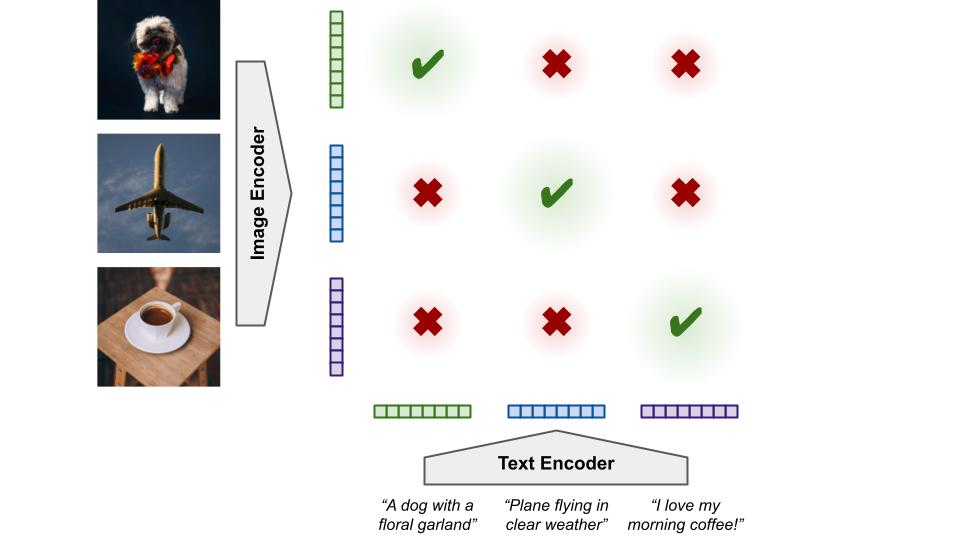
Multimodal contrastive learning trains models to produce similar representations for closely matched images and texts.

This training can be done on noisy, loosely aligned pairs of image and text, which naturally occur on the web. This circumvents the need for manual labeling, and makes data scaling easy. Furthermore, the model learns much richer visual concepts — it’s not constrained to what’s defined in the classification label space. Instead of classifying an image as “coffee”, it can understand whether it’s "a small espresso in a white mug” or “a large latte in a red flask”.

Once trained, a model that aligns image and text can be used in many ways. For zero-shot classification, we compare image representations to text representations of the class names. For example, a “wombat vs jaguar” classifier can be built by computing the representations of the texts “jaguar” and “wombat”, and classifying an image as a jaguar if its representation better matches the former. This approach scales to thousands of classes and makes it very easy to solve classification tasks without the extra data necessary for fine-tuning. Another application of contrastive models is image search (a.k.a. image-text retrieval), by finding the image whose representation best matches that of a given text, or vice versa.

The Best of Both Worlds with Locked-image Tuning
As mentioned earlier, transfer learning achieves state-of-the-art accuracy, but requires per-task labels, datasets, and training. On the other hand, contrastive models are flexible, scalable, and easily adaptable to new tasks, but fall short in performance. To compare, at the time of writing, the state of the art on ImageNet classification using transfer learning is 90.94%, but the best contrastive zero-shot models achieve 76.4%.

LiT tuning bridges this gap: we contrastively train a text model to compute representations well aligned with the powerful ones available from a pre-trained image encoder. Importantly, for this to work well, the image encoder should be “locked“, that is: it should not be updated during training. This may be unintuitive since one usually expects the additional information from further training to increase performance, but we find that locking the image encoder consistently leads to better results.

LiT-tuning contrastively trains a text encoder to match a pre-trained image encoder. The text encoder learns to compute representations that align to those from the image encoder.

This can be considered an alternative to the classic fine-tuning stage, where the image encoder is separately adapted to every new classification task; instead we have one stage of LiT-tuning, after which the model can classify any data. LiT-tuned models achieve 84.5% zero-shot accuracy on ImageNet classification, showing significant improvements over previous methods that train models from scratch, and halving the performance gap between fine-tuning and contrastive learning.

Left: LiT-tuning significantly closes the gap between the best contrastive models and the best models fine-tuned with labels. Right: Using a pre-trained image encoder is always helpful, but locking it is surprisingly a key part of the recipe to success; unlocked image models (dashed) yield significantly worse performance.

An impressive benefit of contrastive models is increased robustness — they retain high accuracy on datasets that typically fool fine-tuned models, such as ObjectNet and ImageNet-C. Similarly, LiT-tuned models have high performance across various challenging versions of ImageNet, for example achieving a state-of-the-art 81.1% accuracy on ObjectNet.

LiT-tuning has other advantages. While prior contrastive works require large amounts of data and train for a very long time, the LiT approach is much less data hungry. LiT models trained on 24M publicly available image-text pairs rival the zero-shot classification performance of prior models trained on 400M image-text pairs of private data. The locked image encoder also leads to faster training with a smaller memory footprint. On larger datasets, image representations can be pre-computed; not running the image model during training further improves efficiency and also unlocks much larger batch sizes, which increases the number of “negatives” the model sees and is key to high-performance contrastive learning. The method works well with varied forms of image pre-training (e.g., including self-supervised learning), and with many publicly available image models. We hope that these benefits make LiT a great testbed for researchers.

Conclusion
We present Locked-image Tuning (LiT), which contrastively trains a text encoder to match image representations from a powerful pre-trained image encoder. This simple method is data and compute efficient, and substantially improves zero-shot classification performance compared to existing contrastive learning approaches.

Want to try it yourself?

A preview of the demo: use it to match free-form text descriptions to images and build your own zero-shot classifier!

We have prepared a small interactive demo to try some LiT-tuned models. We also provide a Colab with more advanced use cases and larger models, which are a great way to get started.

Acknowledgments
We would like to thank Xiaohua Zhai, Xiao Wang, Daniel Keysers, Alexander Kolesnikov, and Lucas Beyer who have co-authored the LiT paper and been involved in all aspects of its development, as well as the Brain team in Zürich. We also would like to thank Tom Small for creating the animations used in this blogpost.

Source: Google AI Blog

Simple and Effective Zero-Shot Task-Oriented Dialogue

Posted by Jeffrey Zhao and Raghav Gupta, Software Engineers, Google Research

Modern conversational agents need to integrate with an ever-increasing number of services to perform a wide variety of tasks, from booking flights and finding restaurants, to playing music and telling jokes. Adding this functionality can be difficult — for each new task, one needs to collect new data and retrain the models that power the conversational agent. This is because most task-oriented dialogue (TOD) models are trained on a single task-specific ontology. An ontology is generally represented as a list of possible user intents (e.g., if the user wants to book a flight, if the user wants to play some music, etc.) and possible parameter slots to extract from the conversation (e.g., the date of the flight, the name of a song, and so on). A rigid ontology can be limiting, preventing the model from generalizing to new tasks or domains. For instance, a TOD model trained on a certain ontology only knows the intents in that ontology, and lacks the ability to generalize its knowledge to unseen intents. This is true even for new ontologies that overlap with ones already known to the agent — for example, if an agent already knows how to book train tickets, adding the ability to book airline tickets would require training on completely new data. Ideally, the agent should be able to leverage its existing knowledge from one ontology, and apply it to new ones.

New benchmarks, such as the the Schema Guided Dialogue (SGD) dataset, have been designed to evaluate the ability to generalize to unseen tasks, by distilling each ontology into a schema of slots and intents. In the SGD setting, TOD models are trained on multiple schemas, and evaluated on how well they generalize to unseen ones — instead of how well they overfit to a single ontology. However, recent work shows the top models still have room for improvement.

To address this problem, we introduce two different sequence-to-sequence approaches toward zero-shot transfer for dialogue modeling, presented in the papers “Description-Driven Task-Oriented Dialogue” and “Show, Don’t Tell: Demonstrations Outperform Descriptions for Schema-Guided Task-Oriented Dialogue”. Both models condition on additional contextual information, either slot and intent descriptions, or single demonstrative examples. Results obtained on multiple dialogue state tracking benchmarks show that by doing away with the fixed schemas and ontologies, these new approaches lead to state-of-the-art results on the dialogue state tracking task with more efficient models. The source code for the described approaches can be found here.

Background: Dialogue State Tracking
To address the challenge of zero-shot transfer for dialogue models, we focus on the problem of Dialogue State Tracking (DST). DST is a fundamental problem for conversational agents, in which a model predicts the belief state of a conversation, i.e., the agent’s understanding of the user’s indicated preferences. The belief state is typically modeled as an assignment of values to slots for which the user has indicated a preference in the conversation. An example is shown below.

An example conversation and its ground truth slots and intents for dialogue state tracking. Here, the active user intent is “Book a train”, and pertinent information for booking this train is recorded in the slot values.

Description-Driven Task-Oriented Dialogue
In our first paper, we introduce Description-Driven Dialogue State Tracking (D3ST), a DST model that leverages slot and intent descriptions when making predictions about the belief state. D3ST is built on top of the T5 sequence-to-sequence language model, which was shown in previous work to be pretrained effectively for DST problems.

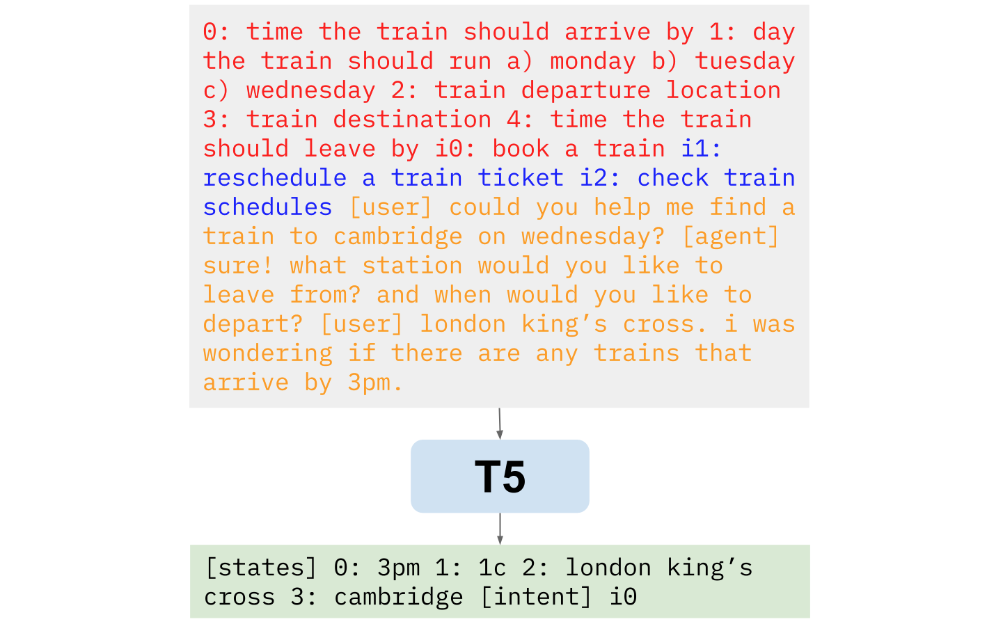
D3ST prompts the input sequence with slot and intent descriptions, allowing the T5 model to attend to both this contextual information and the conversation. Its ability to generalize comes from the formulation of these descriptions. Instead of using a name for each slot, we assign a random index for every slot. For categorical slots (i.e., slots that only take values from a small, predefined set), possible values are also arbitrarily enumerated and then listed. The same is done with intents, and together these descriptions form the schema representation to be included in the input string. This is concatenated with the conversation text and fed into the T5 model. The target output is the belief state and user intent, again identified by their assigned indices. An example is shown below.

An example of the D3ST input and output format. The red text contains slot descriptions, while the blue text contains intent descriptions. The yellow text contains the conversation utterances.

This forces the model to predict conversation contexts using a slot’s index, and not that specific slot. By randomizing the index we assign to each slot between different examples, we prevent the model from learning specific schema information. The slot with index 0 could be the “Train Departure” slot in one example, and the “Train Destination” in another — as such, the model is encouraged to use the slot description given in index 0 to find the correct value, and discouraged from overfitting to a specific schema. With this setup, a model that sees enough different tasks or domains will learn to generalize the action of belief state tracking and intent prediction.

Show Don’t Tell
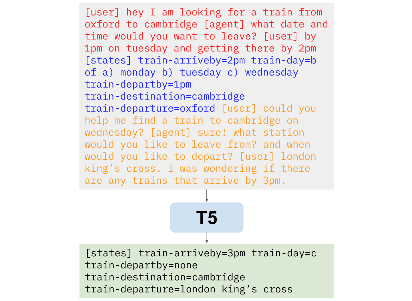
In our subsequent paper, “Show, Don’t Tell: Demonstrations Outperform Descriptions for Schema-Guided Task-Oriented Dialogue”, we employ a single annotated dialogue example that demonstrates the possible slots and values in a conversation, instead of relying on slot descriptions. In this sense, we “show” the semantics of the schema rather than “tell” the model through descriptions — hence the name “Show Don’t Tell” (SDT). SDT is also built on T5, and improves zero-shot performance beyond D3ST.

n example of the SDT input and output format. The text in red contains the demonstrative example, while the text in blue contains its ground truth belief state. The actual conversation for the model to predict is in yellow. While the D3ST prompt relies entirely on slot descriptions, the SDT prompt contains a concise example dialogue followed by the expected dialogue state annotations, resulting in more direct supervision.

The rationale for SDT’s single example demonstration is simple: there can still be ambiguities that are not fully captured in a slot or intent description, and require a concrete example to demonstrate. Moreover, from a developer’s standpoint, creating short dialogue examples to describe a schema can often be easier than writing descriptions that fully capture the meaning behind each slot and intent.

Benchmark Results
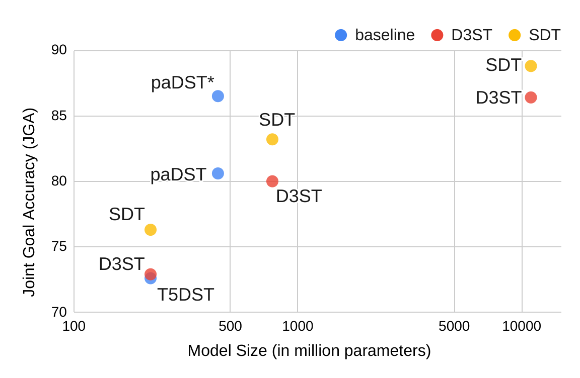
We evaluate both D3ST and SDT on a number of benchmarks, most notably the SGD dataset, which tests zero-shot generalization to unseen schemas in its test set. We evaluate our state tracking models on joint goal accuracy (JGA), the fraction of dialogue turns for which the model predicts an exactly correct belief state.

Both of our models either match or outperform existing state-of-the-art baselines (T5DST and paDST) at comparable model sizes, as shown below. In general, SDT performs slightly better than D3ST. Note that our models can be trained on different sizes of the underlying T5 language model. In addition, while the baseline models can only make predictions for one slot per forward pass, both our models can decode the entire dialogue state in a single forward pass — a much more efficient method in both training and inference.

Joint Goal Accuracy on the SGD dataset plotted against model size for existing baselines and our proposed models D3ST and SDT. Note that paDST* includes additional data augmentation.

Additional metrics are reported in both papers. D3ST exhibits state-of-the-art quality on the MultiWOZ dataset, with 75.9% JGA on MultiWOZ 2.4. Both D3ST and SDT show state-of-the-art performance in the MultiWOZ cross-domain leave-one-out setting. In addition, both D3ST and SDT were evaluated using the SGD-X dataset, and demonstrated strong robustness to linguistic variations in schema. These benchmarks all indicate that D3ST and SDT are state-of-the-art TOD models, with the ability to generalize to unseen tasks and domains.

Zero-Shot Capability
D3ST and SDT sometimes demonstrate a surprising ability to generalize to unseen tasks, and we saw many interesting examples when trying completely new dialogues with the model. We’ve included one such example below:

A D3ST model trained on the SGD dataset makes predictions (right) for an unseen meta conversation (left) about creating this blog post. The model predicts a completely correct belief state, even though it is not fine-tuned on anything related to blogs, authors or NLP.

Future Work
These papers demonstrate the feasibility of a zero-shot TOD system that can generalize to unseen tasks or domains. However, we’ve limited ourselves to the DST problem for now — we plan to extend this research to enable zero-shot dialogue policy modeling, allowing TOD systems to take actions following arbitrary instructions. In addition, the current input format can often lead to long input sequences, which can be slow for inference — we’re exploring new and more efficient methods to encode schema information.

Acknowledgements
This post reflects the combined work of Jeffrey Zhao, Raghav Gupta, Harrison Lee, Mingqiu Wang, Dian Yu, Yuan Cao, and Abhinav Rastogi. We’d like to thank Yonghui Wu and Izhak Shafran for their continued advice and guidance.

Source: Google AI Blog

Lidar-Camera Deep Fusion for Multi-Modal 3D Detection

Posted by Yingwei Li, Student Researcher, Google Cloud and Adams Wei Yu, Research Scientist, Google Research, Brain Team

LiDAR and visual cameras are two types of complementary sensors used for 3D object detection in autonomous vehicles and robots. LiDAR, which is a remote sensing technique that uses light in the form of a pulsed laser to measure ranges, provides low-resolution shape and depth information, while cameras provide high-resolution shape and texture information. While the features captured by LiDAR and cameras should be merged together to provide optimal 3D object detection, it turns out that most state-of-the-art 3D object detectors use LiDAR as the only input. The main reason is that to develop robust 3D object detection models, most methods need to augment and transform the data from both modalities, making the accurate alignment of the features challenging.

Existing algorithms for fusing LiDAR and camera outputs, such as PointPainting, PointAugmenting, EPNet, 4D-Net and ContinuousFusion, generally follow two approaches — input-level fusion where the features are fused at an early stage, decorating points in the LiDAR point cloud with the corresponding camera features, or mid-level fusion where features are extracted from both sensors and then combined. Despite realizing the importance of effective alignment, these methods struggle to efficiently process the common scenario where features are enhanced and aggregated before fusion. This indicates that effectively fusing the signals from both sensors might not be straightforward and remains challenging.

In our CVPR 2022 paper, “DeepFusion: LiDAR-Camera Deep Fusion for Multi-Modal 3D Object Detection”, we introduce a fully end-to-end multi-modal 3D detection framework called DeepFusion that applies a simple yet effective deep-level feature fusion strategy to unify the signals from the two sensing modalities. Unlike conventional approaches that decorate raw LiDAR point clouds with manually selected camera features, our method fuses the deep camera and deep LiDAR features in an end-to-end framework. We begin by describing two novel techniques, InverseAug and LearnableAlign, that improve the quality of feature alignment and are applied to the development of DeepFusion. We then demonstrate state-of-the-art performance by DeepFusion on the Waymo Open Dataset, one of the largest datasets for automotive 3D object detection.

InverseAug: Accurate Alignment under Geometric Augmentation
To achieve good performance on existing 3D object detection benchmarks for autonomous cars, most methods require strong data augmentation during training to avoid overfitting. However, the necessity of data augmentation poses a non-trivial challenge in the DeepFusion pipeline. Specifically, the data from the two modalities use different augmentation strategies, e.g., rotating along the z-axis for 3D point clouds combined with random flipping for 2D camera images, often resulting in alignment that is inaccurate. Then the augmented LiDAR data has to go through a voxelization step that converts the point clouds into volume data stored in a three dimensional array of voxels. The voxelized features are quite different compared to the raw data, making the alignment even more difficult. To address the alignment issue caused by geometry-related data augmentation, we introduce Inverse Augmentation (InverseAug), a technique used to reverse the augmentation before fusion during the model’s training phase.

In the example below, we demonstrate the difficulties in aligning the augmented LiDAR data with the camera data. In this case, the LiDAR point cloud is augmented by rotation with the result that a given 3D key point, which could be any 3D coordinate, such as a LiDAR data point, cannot be easily aligned in 2D space simply through use of the original LiDAR and camera parameters. To make the localization feasible, InverseAug first stores the augmentation parameters before applying the geometry-related data augmentation. At the fusion stage, it reverses all data augmentation to get the original coordinate for the 3D key point, and then finds its corresponding 2D coordinates in the camera space.

During training, InverseAug resolves the inaccurate alignment from geometric augmentation.

Left: Alignment without InverseAug. Right: Alignment quality improvement with InverseAug.

LearnableAlign: A Cross-Modality-Attention Module to Learn Alignment
We also introduce Learnable Alignment (LearnableAlign), a cross-modality-attention–based feature-level alignment technique, to improve the alignment quality. For input-level fusion methods, such as PointPainting and PointAugmenting, given a 3D LiDAR point, only the corresponding camera pixel can be exactly located as there is a one-to-one mapping. In contrast, when fusing deep features in the DeepFusion pipeline, each LiDAR feature represents a voxel containing a subset of points, and hence, its corresponding camera pixels are in a polygon. So the alignment becomes the problem of learning the mapping between a voxel cell and a set of pixels.

A naïve approach is to average over all pixels corresponding to the given voxel. However, intuitively, and as supported by our visualized results, these pixels are not equally important because the information from the LiDAR deep feature unequally aligns with every camera pixel. For example, some pixels may contain critical information for detection (e.g., the target object), while others may be less informative (e.g., consisting of backgrounds such as roads, plants, occluders, etc.).

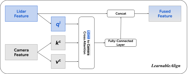
LearnableAlign leverages a cross-modality attention mechanism to dynamically capture the correlations between two modalities. Here, the input contains the LiDAR features in a voxel cell, and all its corresponding camera features. The output of the attention is essentially a weighted sum of the camera features, where the weights are collectively determined by a function of the LiDAR and camera features. More specifically, LearnableAlign uses three fully-connected layers to respectively transform the LiDAR features to a vector (q^l), and camera features to vectors (k^c) and (v^c). For each vector (q^l), we compute the dot products between (q^l) and (k^c) to obtain the attention affinity matrix that contains correlations between the LiDAR features and the corresponding camera features. Normalized by a softmax operator, the attention affinity matrix is then used to calculate weights and aggregate the vectors (v^c) that contain camera information. The aggregated camera information is then processed by a fully-connected layer, and concatenated (Concat) with the original LiDAR feature. The output is then fed into any standard 3D detection framework, such as PointPillars or CenterPoint for model training.

LearnableAlign leverages the cross-attention mechanism to align LiDAR and camera features.

DeepFusion: A Better Way to Fuse Information from Different Modalities
Powered by our two novel feature alignment techniques, we develop DeepFusion, a fully end-to-end multi-modal 3D detection framework. In the DeepFusion pipeline, the LiDAR points are first fed into an existing feature extractor (e.g., pillar feature net from PointPillars) to obtain LiDAR features (e.g., pseudo-images). In the meantime, the camera images are fed into a 2D image feature extractor (e.g., ResNet) to obtain camera features. Then, InverseAug and LearnableAlign are applied in order to fuse the camera and LiDAR features together. Finally, the fused features are processed by the remaining components of the selected 3D detection model (e.g., the backbone and detection head from PointPillars) to obtain the detection results.

The pipeline of DeepFusion.

Benchmark Results
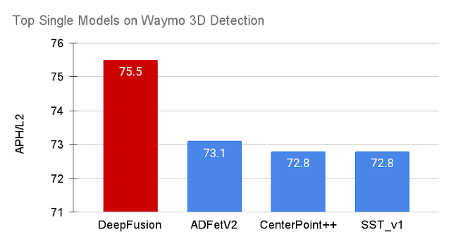
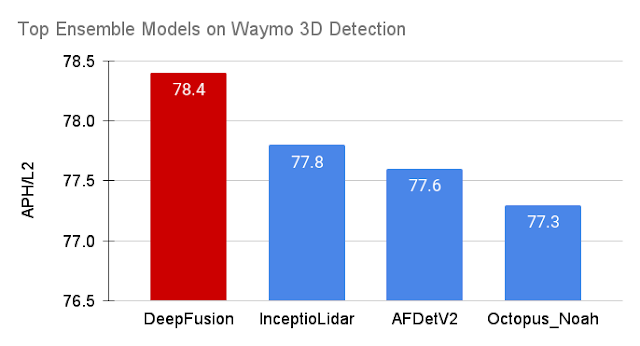
We evaluate DeepFusion on the Waymo Open Dataset, one of the largest 3D detection challenges for autonomous cars, using the Average Precision with Heading (APH) metric under difficulty level 2, the default metric to rank a model’s performance on the leaderboard. Among the 70 participating teams all over the world, the DeepFusion single and ensemble models achieve state-of-the-art performance in their corresponding categories.

The single DeepFusion model achieves new state-of-the-art performance on Waymo Open Dataset.

The Ensemble DeepFusion model outperforms all other methods on Waymo Open Dataset, ranking No. 1 on the leaderboard.

The Impact of InverseAug and LearnableAlign
We also conduct ablation studies on the effectiveness of the proposed InverseAug and LearnableAlign techniques. We demonstrate that both InverseAug and LearnableAlign individually contribute to a performance gain over the LiDAR-only model, and combining both can further yield an even more significant boost.

Ablation studies on InverseAug (IA) and LearnableAlign (LA) measured in average precision (AP) and APH. Combining both techniques contributes to the best performance gain.

Conclusion
We demonstrate that late-stage deep feature fusion can be more effective when features are aligned well, but aligning features from two different modalities can be challenging. To address this challenge, we propose two techniques, InverseAug and LearnableAlign, to improve the quality of alignment among multimodal features. By integrating these techniques into the fusion stage of our proposed DeepFusion method, we achieve state-of-the-art performance on the Waymo Open Dataset.

Acknowledgements:
Special thanks to co-authors Tianjian Meng, Ben Caine, Jiquan Ngiam, Daiyi Peng, Junyang Shen, Bo Wu, Yifeng Lu, Denny Zhou, Quoc Le, Alan Yuille, Mingxing Tan.

Source: Google AI Blog

Large-Scale Matrix Factorization on TPUs

Posted by Harsh Mehta, Software Engineer, Google Research

Matrix factorization is one of the oldest, yet still widely used, techniques for learning how to recommend items such as songs or movies from user ratings. In its basic form, it approximates a large, sparse (i.e., mostly empty) matrix of user-item interactions with a product of two smaller, denser matrices representing learned item and user features. These dense matrices, in turn, can be used to recommend items to a user with which they haven't interacted before.

Despite its algorithmic simplicity, matrix factorization can still achieve competitive performance in recommender benchmarks. Alternating least squares (ALS), and especially its implicit variation, is a fundamental algorithm to learn the parameters of matrix factorization. ALS is known for its high efficiency because it scales linearly in the number of rows, columns and non-zeros. Hence, this algorithm is very well suited for large-scale challenges. But, for very large real-world matrix factorization datasets, a single machine implementation would not suffice, and so, it would require a large distributed system. Most of the distributed implementations of matrix factorization that employ ALS leverage off-the-shelf CPU devices, and rightfully so, due to the inherently sparse nature of the problem (the input matrix is mostly empty).

On the other hand, recent success of deep learning, which has exhibited growing computational capacity, has spurred a new wave of research and progress on hardware accelerators such as Tensor Processing Units (TPUs). TPUs afford domain specific hardware speedups, especially for use cases like deep learning, which involves a large number of dense matrix multiplications. In particular, they allow significant speedups for traditional data-parallel workloads, such as training models with Stochastic Gradient Descent (SGD) in SPMD (single program multiple data) fashion. The SPMD approach has gained popularity in computations like training neural networks with gradient descent algorithms, and can be used for both data-parallel and model-parallel computations, where we distribute parameters of the model across available devices. Nevertheless, while TPUs have been enormously attractive for methods based on SGD, it is not immediately clear if a high performance implementation of ALS, which requires a large number of distributed sparse matrix multiplies, can be developed for a large-scale cluster of TPU devices.

In “ALX: Large Scale Matrix Factorization on TPUs”, we explore a distributed ALS design that makes efficient use of the TPU architecture and can scale well to matrix factorization problems of the order of billions of rows and columns by scaling the number of available TPU cores. The approach we propose leverages a combination of model and data parallelism, where each TPU core both stores a portion of the embedding table and trains over a unique slice of data, grouped in mini-batches. In order to spur future research on large-scale matrix factorization methods and to illustrate the scalability properties of our own implementation, we also built and released a real world web link prediction dataset called WebGraph.

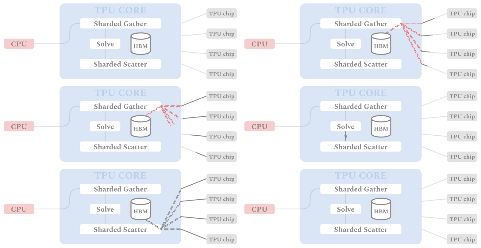
The figure shows the flow of data and computation through the ALX framework on TPU devices. Similar to SGD-based training procedures, each TPU core performs identical computation for its own batch of data in SPMD fashion, which allows for synchronous computation in parallel on multiple TPU cores. Each TPU starts with gathering all the relevant item embeddings in the Sharded Gather stage. These materialized embeddings are used to solve for user embeddings which are scattered to the relevant shard of the embedding table in the Sharded Scatter stage.

Dense Batching for Improved Efficiency
We designed ALX specifically for TPUs, exploiting unique properties of TPU architecture while overcoming a few interesting limitations. For instance, each TPU core has limited memory and restricts all tensors to have a static shape, but each example in a mini-batch can have a wildly varying number of items (i.e., inputs can be long and sparse). To resolve this, we break exceedingly long examples into multiple smaller examples of the same shape, a process called dense batching. More details about dense batching can be found in our paper.

Illustrating example of how sparse batches are densified to increase efficiency on TPUs.

Uniform Sharding of Embedding Tables
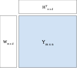
With the batching problem solved, we next want to factorize a sparse matrix into two dense embedding matrices (e.g., user and item embeddings) such that the resulting dot product of embeddings approximate the original sparse matrix — this helps us infer predictions for all the positions from the original matrix, including those that were empty, which can be used to recommend items with which users haven’t interacted. Both the resulting embedding tables (W and H in the figure below) can potentially be too large to fit in a single TPU core, thus requiring a distributed training setup for most large-scale use cases.

Most previous attempts of distributed matrix factorization use a parameter server architecture where the model parameters are stored on highly available servers, and the training data is processed in parallel by workers that are solely responsible for the learning task. In our case, since each TPU core has identical compute and memory, it's wasteful to only use either memory for storing model parameters or compute for training. Thus, we designed our system such that each core is used to do both.

Illustrative example of factorizing a sparse matrix Y into two dense embedding matrices W and H.

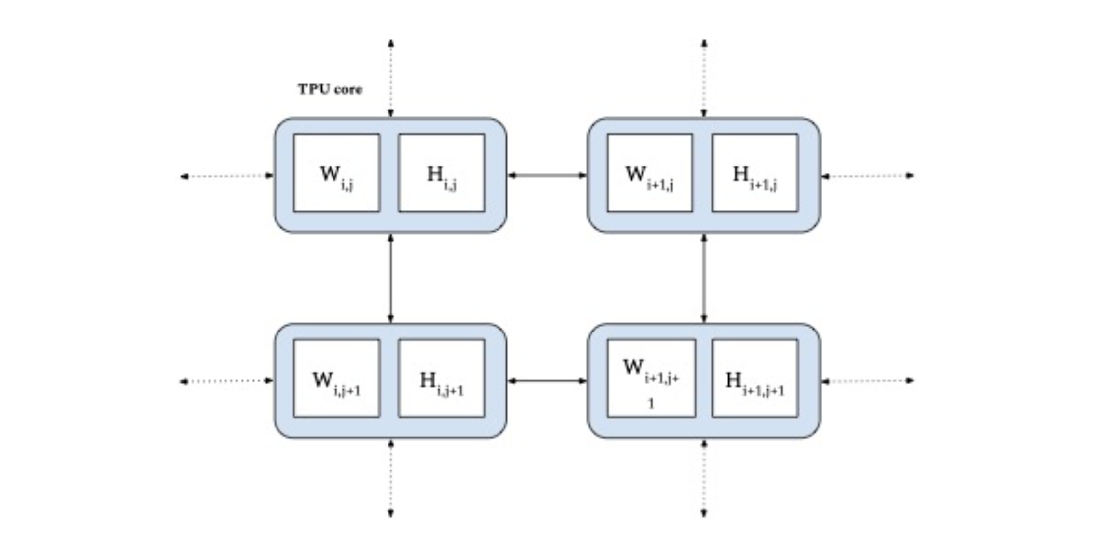
In ALX, we uniformly divide both embedding tables, thus fully exploiting both the size of distributed memory available and the dedicated low-latency interconnects between TPUs. This is highly efficient for very large embedding tables and results in good performance for distributed gather and scatter operations.

Uniform sharding of both embedding tables (W and H) across TPU cores (in blue).

WebGraph
Since potential applications may involve very large data sets, scalability is potentially an important opportunity for advancement in matrix factorization. To that end, we also release a large real-world web link prediction dataset called WebGraph. This dataset can be easily modeled as a matrix factorization problem where rows and columns are source and destination links, respectively, and the task is to predict destination links from each source link. We use WebGraph to illustrate the scaling properties of ALX.

The WebGraph dataset was generated from a single crawl performed by CommonCrawl in 2021 where we strip everything and keep only the link->outlinks data. Since the performance of a factorization method depends on the properties of the underlying graph, we created six versions of WebGraph, each varying in the sparsity pattern and locale, to study how well ALS performs on each.

To study locale-specific graphs, we filter based on two top level domains: ‘de’ and ‘in’, each producing a graph with an order of magnitude fewer nodes.
These graphs can still have arbitrary sparsity patterns and dangling links. Thus we further filter the nodes in each graph to have a minimum of either 10 or 50 inlinks and outlinks.

For easy access, we have made these available as a Tensorflow Dataset package. For reference, the biggest version, WebGraph-sparse, has more than 365M nodes and 30B edges. We create and publish both training and testing splits for evaluation purposes.

Results
We carefully tune the system and quality parameters of ALX. Based on our observations related to precision and choice of linear solvers. We observed that by carefully selecting the precision for storage of the embedding tables (bfloat16) and for the input to the linear solvers (float32), we were able to halve the memory required for the embeddings while still avoiding problems arising from lower precision values during the solve stage. For our linear solvers, we selected conjugate gradients, which we found to be the fastest across the board on TPUs. We use embeddings of dimension 128 and train the model for 16 epochs. In our experience, hyperparameter tuning over both norm penalty (λ) and unobserved weight (α) has been indispensable for good recall metrics as shown in the table below.

Results obtained by running ALX on all versions of WebGraph dataset. Recall values of 1.0 denote perfect recall.

Scaling Analysis
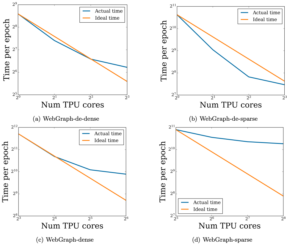
Since the input data are processed in parallel across TPU cores, increasing the number of cores decreases training time, ideally in a linear fashion. But at the same time, a larger number of cores requires more network communication (due to the sharded embedding tables). Thanks to high-speed interconnects, this overhead can be negligible for a small number of cores, but as the number of cores increases, the overhead eventually slows down the ideal linear scaling.

In order to confirm our hypothesis, we analyze scaling properties of the four biggest WebGraph variants in terms of training time as we increase the number of available TPU cores. As shown below, even empirically, we do observe the predicted linear decrease in training time up to a sweet spot, after which the network overhead slows the decline.

Scaling analysis of running time as the number of TPU cores are increased. Each figure plots the time taken to train for one epoch in seconds.

Conclusion
For easy access and reproducibility, the ALX code is open-sourced and can be easily run on Google Cloud. In fact, we illustrate that a sparse matrix like WebGraph-dense of size 135M x 135M (with 22B edges) can be factorized in a colab connected to 8 TPU cores in less than a day. We have designed the ALX framework with scalability in mind. With 256 TPU cores, one epoch of the largest WebGraph variant, WebGraph-sparse (365M x 365M sparse matrix) takes around 20 minutes to finish (5.5 hours for the whole training run). The final model has around 100B parameters. We hope that the ALX and WebGraph will be useful to both researchers and practitioners working in these fields. The code for ALX can be found here on github!

Acknowledgements
The core team includes Steffen Rendle, Walid Krichene and Li Zhang. We thank many Google colleagues for helping at various stages of this project. In particular, we are grateful to the JAX team for numerous discussions, especially James Bradbury and Skye Wanderman-Milne; Blake Hechtman for help with XLA and Rasmus Larsen for useful discussions about performance of linear solvers on TPUs. Finally, we're also grateful to Nicolas Mayoraz, John Anderson, and Fernando Pereira for providing useful feedback.

Source: Google AI Blog

VDTTS: Visually-Driven Text-To-Speech

Posted by Tal Remez, Software Engineer, Google Research and Micheal Hassid, Software Engineer Intern, Google Research

Recent years have seen a tremendous increase in the creation and serving of video content to users across the world in a variety of languages and over numerous platforms. The process of creating high quality content can include several stages from video capturing and captioning to video and audio editing. In some cases dialogue is re-recorded (referred to as dialog replacement, post-sync or dubbing) in a studio in order to achieve high quality and replace original audio that might have been recorded in noisy conditions. However, the dialog replacement process can be difficult and tedious because the newly recorded audio needs to be well synced with the video, requiring several edits to match the exact timing of mouth movements.

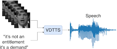
In “More than Words: In-the-Wild Visually-Driven Prosody for Text-to-Speech”, we present a proof-of-concept visually-driven text-to-speech model, called VDTTS, that automates the dialog replacement process. Given a text and the original video frames of the speaker, VDTTS is trained to generate the corresponding speech. As opposed to standard visual speech recognition models, which focus on the mouth region, we detect and crop full faces using MediaPipe to avoid potentially excluding information pertinent to the speaker’s delivery. This gives the VDTTS model enough information to generate speech that matches the video while also recovering aspects of prosody, such as timing and emotion. Despite not being explicitly trained to generate speech that is synchronized to the input video, the learned model still does so.

Given a text and video frames of a speaker, VDTTS generates speech with prosody that matches the video signal.

VDTTS Model
The VDTTS model resembles Tacotron at its core and has four main components: (1) text and video encoders that process the inputs; (2) a multi-source attention mechanism that connects encoders to a decoder; (3) a spectrogram decoder that incorporates the speaker embedding (similarly to VoiceFilter), and produces mel-spectrograms (which are a form of compressed representation in the frequency domain); and (4) a frozen, pretrained neural vocoder that produces waveforms from the mel-spectrograms.

The overall architecture of VDTTS. Text and video encoders process the inputs and then a multisource attention mechanism connects these to a decoder that produces mel-spectrograms. A vocoder then produces waveforms from the mel-spectrograms to generate speech as an output.

We train VDTTS using video and text pairs from LSVSR in which the text corresponds to the exact words spoken by a person in a video. Throughout our testing, we have determined that VDTTS cannot generate arbitrary text, thus making it less prevalent for misuse (e.g., the generation of fake content).

Quality
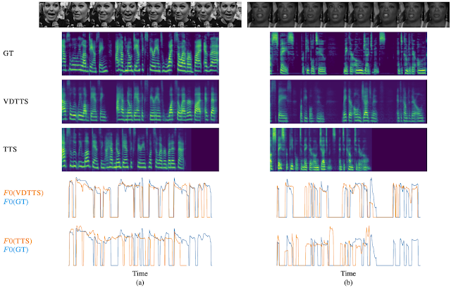
To showcase the unique strength of VDTTS in this post, we have selected two inference examples from the VoxCeleb2 test dataset and compare the performance of VDTTS to a standard text-to-speech (TTS) model. In both examples, the video frames provide prosody and word timing clues, visual information that is not available to the TTS model.

In the first example, the speaker talks at a particular pace that can be seen as periodic gaps in the ground-truth mel-spectrogram (shown below). VDTTS preserves this characteristic and generates audio that is much closer to the ground-truth than the audio generated by standard TTS without access to the video.

Similarly, in the second example, the speaker takes long pauses between some of the words. These pauses are captured by VDTTS and are reflected in the video below, whereas the TTS does not capture this aspect of the speaker’s rhythm.

We also plot fundamental frequency (F0) charts to compare the pitch generated by each model to the ground-truth pitch. In both examples, the F0 curve of VDTTS fits the ground-truth much better than the TTS curve, both in the alignment of speech and silence, and also in how the pitch changes over time. See more original videos and VDTTS generated videos.

We present two examples, (a) and (b), from the VoxCeleb2 test set. From top to bottom: input face images, ground-truth (GT) mel-spectrogram, mel-spectrogram output of VDTTS, mel-spectrogram output of a standard TTS model, and two plots showing the normalized F0 (normalized by mean non-zero pitch, i.e., mean is only over voiced periods) of VDTTS and TTS compared to the ground-truth signal.

Video Samples

Original	VDTTS	VDTTS video-only	TTS

Original displays the original video clip. VDTTS, displays the audio predicted using both the video frames and the text as input. VDTTS video-only displays audio predictions using video frames only. TTS displays audio predictions using text only. Top transcript: "of space for people to make their own judgments and to come to their own". Bottom transcript: "absolutely love dancing I have no dance experience whatsoever but as that".

Model Performance
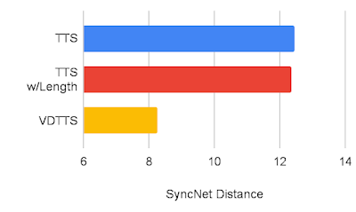
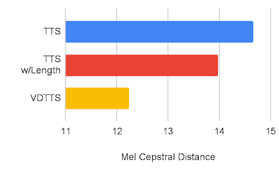
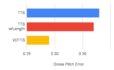
We’ve measured the VDTTS model’s performance using the VoxCeleb2 dataset and compared it to TTS and the TTS with length hint (a TTS that receives the scene length) models. We demonstrate that VDTTS outperforms both models by large margins in most of the aspects we measured: higher sync-to-video quality (measured by SyncNet Distance) and better speech quality as measured by mel cepstral distance (MCD), and lower Gross Pitch Error (GPE), which measures the percentage of frames where pitch differed by more than 20% on frames for which voice was present on both the predicted and reference audio.

SyncNet distance comparison between VDTTS, TTS and the TTS with Length hint (a lower metric is better).

Mel cepstral distance comparison between VDTTS, TTS and the TTS with Length hint (a lower metric is better).

Gross Pitch Error comparison between VDTTS, TTS and the TTS with Length hint (a lower metric is better).

Discussion and Future Work
One thing to note is that, intriguingly, VDTTS can produce video synchronized speech without any explicit losses or constraints to promote this, suggesting complexities such as synchronization losses or explicit modeling are unnecessary.

While this is a proof-of-concept demonstration, we believe that in the future, VDTTS can be upgraded to be used in scenarios where the input text differs from the original video signal. This kind of a model would be a valuable tool for tasks such as translation dubbing.

Acknowledgements
We would like to thank the co-authors of this research: Michelle Tadmor Ramanovich, Ye Jia, Brendan Shillingford, and Miaosen Wang. We are also grateful to the valued contributions, discussions, and feedback from Nadav Bar, Jay Tenenbaum, Zach Gleicher, Paul McCartney, Marco Tagliasacchi, and Yoni Tzafir.

Source: Google AI Blog

Efficiently Initializing Reinforcement Learning With Prior Policies

Posted by Ikechukwu Uchendu, AI Resident and Ted Xiao, Software Engineer, Robotics at Google

Reinforcement learning (RL) can be used to train a policy to perform a task via trial and error, but a major challenge in RL is learning policies from scratch in environments with hard exploration challenges. For example, consider the setting depicted in the door-binary-v0 environment from the adroit manipulation suite, where an RL agent must control a hand in 3D space to open a door placed in front of it.

An RL agent must control a hand in 3D space to open a door placed in front of it. The agent receives a reward signal only when the door is completely open.

Since the agent receives no intermediary rewards, it cannot measure how close it is to completing the task, and so must explore the space randomly until it eventually opens the door. Given how long the task takes and the precise control required, this is extremely unlikely.

For tasks like this, we can avoid exploring the state space randomly by using prior information. This prior information helps the agent understand which states of the environment are good, and should be further explored. We could use offline data (i.e., data collected by human demonstrators, scripted policies, or other RL agents) to train a policy, then use it to initialize a new RL policy. In the case where we use neural networks to represent the policies, this would involve copying the pre-trained policy’s neural network over to the new RL policy. This procedure makes the new RL policy behave like the pre-trained policy. However, naïvely initializing a new RL policy like this often works poorly, especially for value-based RL methods, as shown below.

A policy is pre-trained on the antmaze-large-diverse-v0 D4RL environment with offline data (negative steps correspond to pre-training). We then use the policy to initialize actor-critic fine-tuning (positive steps starting from step 0) with this pre-trained policy as the initial actor. The critic is initialized randomly. The actor’s performance immediately drops and does not recover, as the untrained critic provides a poor learning signal and causes the good initial policy to be forgotten.

With the above in mind, in “Jump-Start Reinforcement Learning” (JSRL), we introduce a meta-algorithm that can use a pre-existing policy of any form to initialize any type of RL algorithm. JSRL uses two policies to learn tasks: a guide-policy, and an exploration-policy. The exploration-policy is an RL policy that is trained online with new experience that the agent collects from the environment, and the guide-policy is a pre-existing policy of any form that is not updated during online training. In this work, we focus on scenarios where the guide-policy is learned from demonstrations, but many other kinds of guide-policies can be used. JSRL creates a learning curriculum by rolling in the guide-policy, which is then followed by the self-improving exploration-policy, resulting in performance that compares to or improves on competitive IL+RL methods.

The JSRL Approach
The guide-policy can take any form: it could be a scripted policy, a policy trained with RL, or even a live human demonstrator. The only requirements are that the guide-policy is reasonable (i.e., better than random exploration), and it can select actions based on observations of the environment. Ideally, the guide-policy can reach poor or medium performance in the environment, but cannot further improve itself with additional fine-tuning. JSRL then allows us to leverage the progress of this guide-policy to take the performance even higher.

At the beginning of training, we roll out the guide-policy for a fixed number of steps so that the agent is closer to goal states. The exploration-policy then takes over and continues acting in the environment to reach these goals. As the performance of the exploration-policy improves, we gradually reduce the number of steps that the guide-policy takes, until the exploration-policy takes over completely. This process creates a curriculum of starting states for the exploration-policy such that in each curriculum stage, it only needs to learn to reach the initial states of prior curriculum stages.

Here, the task is for the robot arm to pick up the blue block. The guide-policy can move the arm to the block, but it cannot pick it up. It controls the agent until it grips the block, then the exploration-policy takes over, eventually learning to pick up the block. As the exploration-policy improves, the guide-policy controls the agent less and less.

Comparison to IL+RL Baselines
Since JSRL can use a prior policy to initialize RL, a natural comparison would be to imitation and reinforcement learning (IL+RL) methods that train on offline datasets, then fine-tune the pre-trained policies with new online experience. We show how JSRL compares to competitive IL+RL methods on the D4RL benchmark tasks. These tasks include simulated robotic control environments, along with datasets of offline data from human demonstrators, planners, and other learned policies. Out of the D4RL tasks, we focus on the difficult ant maze and adroit dexterous manipulation environments.

Example ant maze (left) and adroit dexterous manipulation (right) environments.

For each experiment, we train on an offline dataset and then run online fine-tuning. We compare against algorithms designed specifically for each setting, which include AWAC, IQL, CQL, and behavioral cloning. While JSRL can be used in combination with any initial guide-policy or fine-tuning algorithm, we use our strongest baseline, IQL, as a pre-trained guide and for fine-tuning. The full D4RL dataset includes one million offline transitions for each ant maze task. Each transition is a sequence of format (S, A, R, S’) which specifies what state the agent started in (S), the action the agent took (A), the reward the agent received (R), and the state the agent ended up in (S’) after taking action A. We find that JSRL performs well with as few as ten thousand offline transitions.

Average score (max=100) on the antmaze-medium-diverse-v0 environment from the D4RL benchmark suite. JSRL can improve even with limited access to offline transitions.

Vision-Based Robotic Tasks
Utilizing offline data is especially challenging in complex tasks such as vision-based robotic manipulation due to the curse of dimensionality. The high dimensionality of both the continuous-control action space and the pixel-based state space present scaling challenges for IL+RL methods in terms of the amount of data required to learn good policies. To study how JSRL scales to such settings, we focus on two difficult simulated robotic manipulation tasks: indiscriminate grasping (i.e., lifting any object) and instance grasping (i.e., lifting a specific target object).

A simulated robot arm is placed in front of a table with various categories of objects. When the robot lifts any object, a sparse reward is given for the indiscriminate grasping task. For the instance grasping task, a sparse reward is only given when a specific target object is grasped.

We compare JSRL against methods that are able to scale to complex vision-based robotics settings, such as QT-Opt and AW-Opt. Each method has access to the same offline dataset of successful demonstrations and is allowed to run online fine-tuning for up to 100,000 steps.

In these experiments, we use behavioral cloning as a guide-policy and combine JSRL with QT-Opt for fine-tuning. The combination of QT-Opt+JSRL improves faster than all other methods while achieving the highest success rate.

Mean grasping success for indiscriminate and instance grasping environments using 2k successful demonstrations.

Conclusion
We proposed JSRL, a method for leveraging a prior policy of any form to improve exploration for initializing RL tasks. Our algorithm creates a learning curriculum by rolling in a pre-existing guide-policy, which is then followed by the self-improving exploration-policy. The job of the exploration-policy is greatly simplified since it starts exploring from states closer to the goal. As the exploration-policy improves, the effect of the guide-policy diminishes, leading to a fully capable RL policy. In the future, we plan to apply JSRL to problems such as Sim2Real, and explore how we can leverage multiple guide-policies to train RL agents.

Acknowledgements
This work would not have been possible without Ikechukwu Uchendu, Ted Xiao, Yao Lu, Banghua Zhu, Mengyuan Yan, Joséphine Simon, Matthew Bennice, Chuyuan Fu, Cong Ma, Jiantao Jiao, Sergey Levine, and Karol Hausman. Special thanks to Tom Small for creating the animations for this post.

Source: Google AI Blog

Reproducibility in Deep Learning and Smooth Activations

Posted by Gil Shamir and Dong Lin, Research Software Engineers, Google Research

Ever queried a recommender system and found that the same search only a few moments later or on a different device yields very different results? This is not uncommon and can be frustrating if a person is looking for something specific. As a designer of such a system, it is also not uncommon for the metrics measured to change from design and testing to deployment, bringing into question the utility of the experimental testing phase. Some level of such irreproducibility can be expected as the world changes and new models are deployed. However, this also happens regularly as requests hit duplicates of the same model or models are being refreshed.

Lack of replicability, where researchers are unable to reproduce published results with a given model, has been identified as a challenge in the field of machine learning (ML). Irreproducibility is a related but more elusive problem, where multiple instances of a given model are trained on the same data under identical training conditions, but yield different results. Only recently has irreproducibility been identified as a difficult problem, but due to its complexity, theoretical studies to understand this problem are extremely rare.

In practice, deep network models are trained in highly parallelized and distributed environments. Nondeterminism in training from random initialization, parallelism, distributed training, data shuffling, quantization errors, hardware types, and more, combined with objectives with multiple local optima contribute to the problem of irreproducibility. Some of these factors, such as initialization, can be controlled, but it is impractical to control others. Optimization trajectories can diverge early in training by following training examples in the order seen, leading to very different models. Several recently published solutions [1, 2, 3] based on advanced combinations of ensembling, self-ensembling, and distillation can mitigate the problem, but usually at the cost of accuracy and increased complexity, maintenance and improvement costs.

In “Real World Large Scale Recommendation Systems Reproducibility and Smooth Activations”, we consider a different practical solution to this problem that does not incur the costs of other solutions, while still improving reproducibility and yielding higher model accuracy. We discover that the Rectified Linear Unit (ReLU), which is very popular as the nonlinearity function (i.e., activation function) used to transform values in neural networks, exacerbates the irreproducibility problem. On the other hand, we demonstrate that smooth activation functions, which have derivatives that are continuous for the whole domain, unlike those of ReLU, are able to substantially reduce irreproducibility levels. We then propose the Smooth reLU (SmeLU) activation function, which gives comparable reproducibility and accuracy benefits to other smooth activations but is much simpler.

The ReLU function (left) as function of the input signal, and its gradient (right) as function of the input.

Smooth Activations
An ML model attempts to learn the best model parameters that fit the training data by minimizing a loss, which can be imagined as a landscape with peaks and valleys, where the lowest point attains an optimal solution. For deep models, the landscape may consist of many such peaks and valleys. The activation function used by the model governs the shape of this landscape and how the model navigates it.

ReLU, which is not a smooth function, imposes an objective whose landscape is partitioned into many regions with multiple local minima, each providing different model predictions. With this landscape, the order in which updates are applied is a dominant factor in determining the optimization trajectory, providing a recipe for irreproducibility. Because of its non-continuous gradient, functions expressed by a ReLU network will contain sudden jumps in the gradient, which can occur internally in different layers of the deep network, affecting updates of different internal units, and are likely strong contributors to irreproducibility.

Suppose a sequence of model updates attempts to push the activation of some unit down from a positive value. The gradient of the ReLU function is 1 for positive unit values, so with every update it pushes the unit to become smaller and smaller (to the left in the panel above). At the point the activation of this unit crosses the threshold from a positive value to a negative one, the gradient suddenly changes from magnitude 1 to magnitude 0. Training attempts to keep moving the unit leftwards, but due to the 0 gradient, the unit cannot move further in that direction. Therefore, the model must resort to updating other units that can move.

We find that networks with smooth activations (e.g., GELU, Swish and Softplus) can be substantially more reproducible. They may exhibit a similar objective landscape, but with fewer regions, giving a model fewer opportunities to diverge. Unlike the sudden jumps with ReLU, for a unit with decreasing activations, the gradient gradually reduces to 0, which gives other units opportunities to adjust to the changing behavior. With equal initialization, moderate shuffling of training examples, and normalization of hidden layer outputs, smooth activations are able to increase the chances of converging to the same minimum. Very aggressive data shuffling, however, loses this advantage.

The rate that a smooth activation function transitions between output levels, i.e., its “smoothness”, can be adjusted. Sufficient smoothness leads to improved accuracy and reproducibility. Too much smoothness, though, approaches linear models with a corresponding degradation of model accuracy, thus losing the advantages of using a deep network.

Smooth activations (top) and their gradients (bottom) for different smoothness parameter values β as a function of the input values. β determines the width of the transition region between 0 and 1 gradients. For Swish and Softplus, a greater β gives a narrower region, for SmeLU, a greater β gives a wider region.

Smooth reLU (SmeLU)
Activations like GELU and Swish require complex hardware implementations to support exponential and logarithmic functions. Further, GELU must be computed numerically or approximated. These properties can make deployment error-prone, expensive, or slow. GELU and Swish are not monotonic (they start by slightly decreasing and then switch to increasing), which may interfere with interpretability (or identifiability), nor do they have a full stop or a clean slope 1 region, properties that simplify implementation and may aid in reproducibility.

The Smooth reLU (SmeLU) activation function is designed as a simple function that addresses the concerns with other smooth activations. It connects a 0 slope on the left with a slope 1 line on the right through a quadratic middle region, constraining continuous gradients at the connection points (as an asymmetric version of a Huber loss function).

SmeLU can be viewed as a convolution of ReLU with a box. It provides a cheap and simple smooth solution that is comparable in reproducibility-accuracy tradeoffs to more computationally expensive and complex smooth activations. The figure below illustrates the transition of the loss (objective) surface as we gradually transition from a non-smooth ReLU to a smoother SmeLU. A transition of width 0 is the basic ReLU function for which the loss objective has many local minima. As the transition region widens (SmeLU), the loss surface becomes smoother. If the transition is too wide, i.e., too smooth, the benefit of using a deep network wanes and we approach the linear model solution — the objective surface flattens, potentially losing the ability of the network to express much information.

Loss surfaces (as functions of a 2D input) for two sample loss functions (middle and right) as the activation function’s transition region widens, going from from ReLU to an increasingly smoother SmeLU (left). The loss surface becomes smoother with increasing the smoothness of the SmeLU function.

Performance
SmeLU has benefited multiple systems, specifically recommendation systems, increasing their reproducibility by reducing, for example, recommendation swap rates. While the use of SmeLU results in accuracy improvements over ReLU, it also replaces other costly methods to address irreproducibility, such as ensembles, which mitigate irreproducibility at the cost of accuracy. Moreover, replacing ensembles in sparse recommendation systems reduces the need for multiple lookups of model parameters that are needed to generate an inference for each of the ensemble components. This substantially improves training and inference efficiency.

To illustrate the benefits of smooth activations, we plot the relative prediction difference (PD) as a function of change in some loss for the different activations. We define relative PD as the ratio between the absolute difference in predictions of two models and their expected prediction, averaged over all evaluation examples. We have observed that in large scale systems, it is sufficient, and inexpensive, to consider only two models for very consistent results.

The figure below shows curves on the PD-accuracy loss plane. For reproducibility, being lower on the curve is better, and for accuracy, being on the left is better. Smooth activations can yield a ballpark 50% reduction in PD relative to ReLU, while still potentially resulting in improved accuracy. SmeLU yields accuracy comparable to other smooth activations, but is more reproducible (lower PD) while still outperforming ReLU in accuracy.

Relative PD as a function of percentage change in the evaluation ranking loss, which measures how accurately items are ranked in a recommendation system (higher values indicate worse accuracy), for different activations.

Conclusion and Future Work
We demonstrated the problem of irreproducibility in real world practical systems, and how it affects users as well as system and model designers. While this particular issue has been given very little attention when trying to address the lack of replicability of research results, irreproducibility can be a critical problem. We demonstrated that a simple solution of using smooth activations can substantially reduce the problem without degrading other critical metrics like model accuracy. We demonstrate a new smooth activation function, SmeLU, which has the added benefits of mathematical simplicity and ease of implementation, and can be cheap and less error prone.

Understanding reproducibility, especially in deep networks, where objectives are not convex, is an open problem. An initial theoretical framework for the simpler convex case has recently been proposed, but more research must be done to gain a better understanding of this problem which will apply to practical systems that rely on deep networks.

Acknowledgements
We would like to thank Sergey Ioffe for early discussions about SmeLU; Lorenzo Coviello and Angel Yu for help in early adoptions of SmeLU; Shiv Venkataraman for sponsorship of the work; Claire Cui for discussion and support from the very beginning; Jeremiah Willcock, Tom Jablin, and Cliff Young for substantial implementation support; Yuyan Wang, Mahesh Sathiamoorthy, Myles Sussman, Li Wei, Kevin Regan, Steven Okamoto, Qiqi Yan, Todd Phillips, Ed Chi, Sunita Verna, and many many others for many discussions, and for integrations in many different systems; Matt Streeter and Yonghui Wu for feedback on the paper and this post; Tom Small for help with the illustrations in this post.

Source: Google AI Blog

Pathways Language Model (PaLM): Scaling to 540 Billion Parameters for Breakthrough Performance

Posted by Sharan Narang and Aakanksha Chowdhery, Software Engineers, Google Research

In recent years, large neural networks trained for language understanding and generation have achieved impressive results across a wide range of tasks. GPT-3 first showed that large language models (LLMs) can be used for few-shot learning and can achieve impressive results without large-scale task-specific data collection or model parameter updating. More recent LLMs, such as GLaM, LaMDA, Gopher, and Megatron-Turing NLG, achieved state-of-the-art few-shot results on many tasks by scaling model size, using sparsely activated modules, and training on larger datasets from more diverse sources. Yet much work remains in understanding the capabilities that emerge with few-shot learning as we push the limits of model scale.

Last year Google Research announced our vision for Pathways, a single model that could generalize across domains and tasks while being highly efficient. An important milestone toward realizing this vision was to develop the new Pathways system to orchestrate distributed computation for accelerators. In “PaLM: Scaling Language Modeling with Pathways”, we introduce the Pathways Language Model (PaLM), a 540-billion parameter, dense decoder-only Transformer model trained with the Pathways system, which enabled us to efficiently train a single model across multiple TPU v4 Pods. We evaluated PaLM on hundreds of language understanding and generation tasks, and found that it achieves state-of-the-art few-shot performance across most tasks, by significant margins in many cases.

As the scale of the model increases, the performance improves across tasks while also unlocking new capabilities.

Training a 540-Billion Parameter Language Model with Pathways
PaLM demonstrates the first large-scale use of the Pathways system to scale training to 6144 chips, the largest TPU-based system configuration used for training to date. The training is scaled using data parallelism at the Pod level across two Cloud TPU v4 Pods, while using standard data and model parallelism within each Pod. This is a significant increase in scale compared to most previous LLMs, which were either trained on a single TPU v3 Pod (e.g., GLaM, LaMDA), used pipeline parallelism to scale to 2240 A100 GPUs across GPU clusters (Megatron-Turing NLG) or used multiple TPU v3 Pods (Gopher) with a maximum scale of 4096 TPU v3 chips.

PaLM achieves a training efficiency of 57.8% hardware FLOPs utilization, the highest yet achieved for LLMs at this scale. This is due to a combination of the parallelism strategy and a reformulation of the Transformer block that allows for attention and feedforward layers to be computed in parallel, enabling speedups from TPU compiler optimizations.

PaLM was trained using a combination of English and multilingual datasets that include high-quality web documents, books, Wikipedia, conversations, and GitHub code. We also created a “lossless” vocabulary that preserves all whitespace (especially important for code), splits out-of-vocabulary Unicode characters into bytes, and splits numbers into individual tokens, one for each digit.

Breakthrough Capabilities on Language, Reasoning, and Code Tasks
PaLM shows breakthrough capabilities on numerous very difficult tasks. We highlight a few examples for language understanding and generation, reasoning, and code-related tasks below.

Language Understanding and Generation
We evaluated PaLM on 29 widely-used English natural language processing (NLP) tasks. PaLM 540B surpassed few-shot performance of prior large models, such as GLaM, GPT-3, Megatron-Turing NLG, Gopher, Chinchilla, and LaMDA, on 28 of 29 of tasks that span question-answering tasks (open-domain closed-book variant), cloze and sentence-completion tasks, Winograd-style tasks, in-context reading comprehension tasks, common-sense reasoning tasks, SuperGLUE tasks, and natural language inference tasks.

PaLM 540B performance improvement over prior state-of-the-art (SOTA) results on 29 English-based NLP tasks.

In addition to English NLP tasks, PaLM also shows strong performance on multilingual NLP benchmarks, including translation, even though only 22% of the training corpus is non-English.

We also probe emerging and future capabilities of PaLM on the Beyond the Imitation Game Benchmark (BIG-bench), a recently released suite of more than 150 new language modeling tasks, and find that PaLM achieves breakthrough performance. We compare the performance of PaLM to Gopher and Chinchilla, averaged across a common subset of 58 of these tasks. Interestingly, we note that PaLM’s performance as a function of scale follows a log-linear behavior similar to prior models, suggesting that performance improvements from scale have not yet plateaued. PaLM 540B 5-shot also does better than the average performance of people asked to solve the same tasks.

Scaling behavior of PaLM on a subset of 58 BIG-bench tasks.

PaLM demonstrates impressive natural language understanding and generation capabilities on several BIG-bench tasks. For example, the model can distinguish cause and effect, understand conceptual combinations in appropriate contexts, and even guess the movie from an emoji.

Examples that showcase PaLM 540B 1-shot performance on BIG-bench tasks: labeling cause and effect, conceptual understanding, guessing movies from emoji, and finding synonyms and counterfactuals.

Reasoning
By combining model scale with chain-of-thought prompting, PaLM shows breakthrough capabilities on reasoning tasks that require multi-step arithmetic or common-sense reasoning. Prior LLMs, like Gopher, saw less benefit from model scale in improving performance.

Standard prompting versus chain-of-thought prompting for an example grade-school math problem. Chain-of-thought prompting decomposes the prompt for a multi-step reasoning problem into intermediate steps (highlighted in yellow), similar to how a person would approach it.

We observed strong performance from PaLM 540B combined with chain-of-thought prompting on three arithmetic datasets and two commonsense reasoning datasets. For example, with 8-shot prompting, PaLM solves 58% of the problems in GSM8K, a benchmark of thousands of challenging grade school level math questions, outperforming the prior top score of 55% achieved by fine-tuning the GPT-3 175B model with a training set of 7500 problems and combining it with an external calculator and verifier.

This new score is especially interesting, as it approaches the 60% average of problems solved by 9-12 year olds, who are the target audience for the question set. We suspect that separate encoding of digits in the PaLM vocabulary helps enable these performance improvements.

Remarkably, PaLM can even generate explicit explanations for scenarios that require a complex combination of multi-step logical inference, world knowledge, and deep language understanding. For example, it can provide high quality explanations for novel jokes not found on the web.

PaLM explains an original joke with two-shot prompts.

Code Generation
LLMs have also been shown [1, 2, 3, 4] to generalize well to coding tasks, such as writing code given a natural language description (text-to-code), translating code from one language to another, and fixing compilation errors (code-to-code).

PaLM 540B shows strong performance across coding tasks and natural language tasks in a single model, even though it has only 5% code in the pre-training dataset. Its few-shot performance is especially remarkable because it is on par with the fine-tuned Codex 12B while using 50 times less Python code for training. This result reinforces earlier findings that larger models can be more sample efficient than smaller models because they better transfer learning from other programming languages and natural language data.

Examples of a fine-tuned PaLM 540B model on text-to-code tasks, such as GSM8K-Python and HumanEval, and code-to-code tasks, such as Transcoder.

We also see a further increase in performance by fine-tuning PaLM on a Python-only code dataset, which we refer to as PaLM-Coder. For an example code repair task called DeepFix, where the objective is to modify initially broken C programs until they compile successfully, PaLM-Coder 540B demonstrates impressive performance, achieving a compile rate of 82.1%, which outperforms the prior 71.7% state of the art. This opens up opportunities for fixing more complex errors that arise during software development.

An example from the DeepFix Code Repair task. The fine-tuned PaLM-Coder 540B fixes compilation errors (left, in red) to a version of code that compiles (right).

Ethical Considerations
Recent research has highlighted various potential risks associated with LLMs trained on web text. It is crucial to analyze and document such potential undesirable risks through transparent artifacts such as model cards and datasheets, which also include information on intended use and testing. To this end, our paper provides a datasheet, model card and Responsible AI benchmark results, and it reports thorough analyses of the dataset and model outputs for biases and risks. While the analysis helps outline some potential risks of the model, domain- and task-specific analysis is essential to truly calibrate, contextualize, and mitigate possible harms. Further understanding of risks and benefits of these models is a topic of ongoing research, together with developing scalable solutions that can put guardrails against malicious uses of language models.

Conclusion and Future Work
PaLM demonstrates the scaling capability of the Pathways system to thousands of accelerator chips across two TPU v4 Pods by training a 540-billion parameter model efficiently with a well-studied, well-established recipe of a dense decoder-only Transformer model. Pushing the limits of model scale enables breakthrough few-shot performance of PaLM across a variety of natural language processing, reasoning, and code tasks.

PaLM paves the way for even more capable models by combining the scaling capabilities with novel architectural choices and training schemes, and brings us closer to the Pathways vision:

“Enable a single AI system to generalize across thousands or millions of tasks, to understand different types of data, and to do so with remarkable efficiency."

Acknowledgements
PaLM is the result of a large, collaborative effort by many teams within Google Research and across Alphabet. We’d like to thank the entire PaLM team for their contributions: Jacob Devlin, Maarten Bosma, Gaurav Mishra, Adam Roberts, Paul Barham, Hyung Won Chung, Charles Sutton, Sebastian Gehrmann, Parker Schuh, Kensen Shi, Sasha Tsvyashchenko, Joshua Maynez, Abhishek Rao, Parker Barnes, Yi Tay, Noam Shazeer, Vinodkumar Prabhakaran, Emily Reif, Nan Du, Ben Hutchinson, Reiner Pope, James Bradbury, Jacob Austin, Michael Isard, Guy Gur-Ari, Pengcheng Yin, Toju Duke, Anselm Levskaya, Sanjay Ghemawat, Sunipa Dev, Henryk Michalewski, Xavier Garcia, Vedant Misra, Kevin Robinson, Liam Fedus, Denny Zhou, Daphne Ippolito, David Luan, Hyeontaek Lim, Barret Zoph, Alexander Spiridonov, Ryan Sepassi, David Dohan, Shivani Agrawal, Mark Omernick, Andrew Dai, Thanumalayan Sankaranarayana Pillai, Marie Pellat, Aitor Lewkowycz, Erica Moreira, Rewon Child, Oleksandr Polozov, Katherine Lee, Zongwei Zhou, Xuezhi Wang, Brennan Saeta, Mark Diaz, Orhan Firat, Michele Catasta, and Jason Wei. PaLM builds on top of work by many, many teams at Google and we would especially like to recognize the T5X team, the Pathways infrastructure team, the JAX team, the Flaxformer team, the XLA team, the Plaque team, the Borg team, and the Datacenter networking infrastructure team. We’d like to thank our co-authors on this blog post, Alexander Spiridonov and Maysam Moussalem, as well as Josh Newlan and Tom Small for the images and animations in this blog post. Finally, we would like to thank our advisors for the project: Noah Fiedel, Slav Petrov, Jeff Dean, Douglas Eck, and Kathy Meier-Hellstern.

Source: Google AI Blog

Introducing CVSS: A Massively Multilingual Speech-to-Speech Translation Corpus

Posted by Ye Jia and Michelle Tadmor Ramanovich, Software Engineers, Google Research

Automatic translation of speech from one language to speech in another language, called speech-to-speech translation (S2ST), is important for breaking down the communication barriers between people speaking different languages. Conventionally, automatic S2ST systems are built with a cascade of automatic speech recognition (ASR), text-to-text machine translation (MT), and text-to-speech (TTS) synthesis sub-systems, so that the system overall is text-centric. Recently, work on S2ST that doesn’t rely on intermediate text representation is emerging, such as end-to-end direct S2ST (e.g., Translatotron) and cascade S2ST based on learned discrete representations of speech (e.g., Tjandra et al.). While early versions of such direct S2ST systems obtained lower translation quality compared to cascade S2ST models, they are gaining traction as they have the potential both to reduce translation latency and compounding errors, and to better preserve paralinguistic and non-linguistic information from the original speech, such as voice, emotion, tone, etc. However, such models usually have to be trained on datasets with paired S2ST data, but the public availability of such corpora is extremely limited.

To foster research on such a new generation of S2ST, we introduce a Common Voice-based Speech-to-Speech translation corpus, or CVSS, which includes sentence-level speech-to-speech translation pairs from 21 languages into English. Unlike existing public corpora, CVSS can be directly used for training such direct S2ST models without any extra processing. In “CVSS Corpus and Massively Multilingual Speech-to-Speech Translation”, we describe the dataset design and development, and demonstrate the effectiveness of the corpus through training of baseline direct and cascade S2ST models and showing performance of a direct S2ST model that approaches that of a cascade S2ST model.

Building CVSS
CVSS is directly derived from the CoVoST 2 speech-to-text (ST) translation corpus, which is further derived from the Common Voice speech corpus. Common Voice is a massively multilingual transcribed speech corpus designed for ASR in which the speech is collected by contributors reading text content from Wikipedia and other text corpora. CoVoST 2 further provides professional text translation for the original transcript from 21 languages into English and from English into 15 languages. CVSS builds on these efforts by providing sentence-level parallel speech-to-speech translation pairs from 21 languages into English (shown in the table below).

To facilitate research with different focuses, two versions of translation speech in English are provided in CVSS, both are synthesized using state-of-the-art TTS systems, with each version providing unique value that doesn’t exist in other public S2ST corpora:

CVSS-C: All the translation speech is in a single canonical speaker’s voice. Despite being synthetic, the speech is highly natural, clean, and consistent in speaking style. These properties ease the modeling of the target speech and enable trained models to produce high quality translation speech suitable for general user-facing applications where speech quality is of higher importance than accurately reproducing the speakers' voices.
CVSS-T: The translation speech captures the voice from the corresponding source speech. Each S2ST pair has a similar voice on the two sides, despite being in different languages. Because of this, the dataset is suitable for building models where accurate voice preservation is desired, such as for movie dubbing.

Together with the source speech, the two S2ST datasets contain 1,872 and 1,937 hours of speech, respectively.

Source Language	Code	Source speech (X)	CVSS-C target speech (En)	CVSS-T target speech (En)
French	fr	309.3	200.3	222.3
German	de	226.5	137.0	151.2
Catalan	ca	174.8	112.1	120.9
Spanish	es	157.6	94.3	100.2
Italian	it	73.9	46.5	49.2
Persian	fa	58.8	29.9	34.5
Russian	ru	38.7	26.9	27.4
Chinese	zh	26.5	20.5	22.1
Portuguese	pt	20.0	10.4	11.8
Dutch	nl	11.2	7.3	7.7
Estonian	et	9.0	7.3	7.1
Mongolian	mn	8.4	5.1	5.7
Turkish	tr	7.9	5.4	5.7
Arabic	ar	5.8	2.7	3.1
Latvian	lv	4.9	2.6	3.1
Swedish	sv	4.3	2.3	2.8
Welsh	cy	3.6	1.9	2.0
Tamil	ta	3.1	1.7	2.0
Indonesian	id	3.0	1.6	1.7
Japanese	ja	3.0	1.7	1.8
Slovenian	sl	2.9	1.6	1.9
Total		1,153.2	719.1	784.2

Amount of source and target speech of each X-En pair in CVSS (hours).

In addition to translation speech, CVSS also provides normalized translation text matching the pronunciation in the translation speech (on numbers, currencies, acronyms, etc., see data samples below, e.g., where “100%” is normalized as “one hundred percent” or “King George II” is normalized as “king george the second”), which can benefit both model training as well as standardizing the evaluation.

CVSS is released under the Creative Commons Attribution 4.0 International (CC BY 4.0) license and it can be freely downloaded online.

Data Samples

*Example 1:*
Source audio (French)

Source transcript (French)		Le genre musical de la chanson est entièrement le disco.

CVSS-C translation audio (English)
CVSS-T translation audio (English)

Translation text (English)		The musical genre of the song is 100% Disco.

Normalized translation text (English)		the musical genre of the song is one hundred percent disco


*Example 2:*
Source audio (Chinese)

Source transcript (Chinese)		弗雷德里克王子，英国王室成员，为乔治二世之孙，乔治三世之幼弟。

CVSS-C translation audio (English)
CVSS-T translation audio (English)

Translation text (English)		Prince Frederick, member of British Royal Family, Grandson of King George II, brother of King George III.

Normalized translation text (English)		prince frederick member of british royal family grandson of king george the second brother of king george the third

Baseline Models
On each version of CVSS, we trained a baseline cascade S2ST model as well as two baseline direct S2ST models and compared their performance. These baselines can be used for comparison in future research.

Cascade S2ST: To build strong cascade S2ST baselines, we trained an ST model on CoVoST 2, which outperforms the previous states of the art by +5.8 average BLEU on all 21 language pairs (detailed in the paper) when trained on the corpus without using extra data. This ST model is connected to the same TTS models used for constructing CVSS to compose very strong cascade S2ST baselines (ST → TTS).

Direct S2ST: We built two baseline direct S2ST models using Translatotron and Translatotron 2. When trained from scratch with CVSS, the translation quality from Translatotron 2 (8.7 BLEU) approaches that of the strong cascade S2ST baseline (10.6 BLEU). Moreover, when both use pre-training the gap decreases to only 0.7 BLEU on ASR transcribed translation. These results verify the effectiveness of using CVSS to train direct S2ST models.

Translation quality of baseline direct and cascade S2ST models built on CVSS-C, measured by BLEU on ASR transcription from speech translation. The pre-training was done on CoVoST 2 without other extra data sets.

Conclusion
We have released two versions of multilingual-to-English S2ST datasets, CVSS-C and CVSS-T, each with about 1.9K hours of sentence-level parallel S2ST pairs, covering 21 source languages. The translation speech in CVSS-C is in a single canonical speaker’s voice, while the same in CVSS-T is in voices transferred from the source speech. Each of these datasets provides unique value not existing in other public S2ST corpora.

We built baseline multilingual direct S2ST models and cascade S2ST models on both datasets, which can be used for comparison in future works. To build strong cascade S2ST baselines, we trained an ST model on CoVoST 2, which outperforms the previous states of the art by +5.8 average BLEU when trained on the corpus without extra data. Nevertheless, the performance of the direct S2ST models approaches the strong cascade baselines when trained from scratch, and with only 0.7 BLEU difference on ASR transcribed translation when utilized pre-training. We hope this work helps accelerate the research on direct S2ST.

Acknowledgments
We acknowledge the volunteer contributors and the organizers of the Common Voice and LibriVox projects for their contribution and collection of recordings, the creators of Common Voice, CoVoST, CoVoST 2, Librispeech and LibriTTS corpora for their previous work. The direct contributors to the CVSS corpus and the paper include Ye Jia, Michelle Tadmor Ramanovich, Quan Wang, Heiga Zen. We also thank Ankur Bapna, Yiling Huang, Jason Pelecanos, Colin Cherry, Alexis Conneau, Yonghui Wu, Hadar Shemtov and Françoise Beaufays for helpful discussions and support.

Source: Google AI Blog

Introducing CVSS: A Massively Multilingual Speech-to-Speech Translation Corpus

Posted by Ye Jia and Michelle Tadmor Ramanovich, Software Engineers, Google Research

CVSS-C: All the translation speech is in a single canonical speaker’s voice. Despite being synthetic, the speech is highly natural, clean, and consistent in speaking style. These properties ease the modeling of the target speech and enable trained models to produce high quality translation speech suitable for general user-facing applications where speech quality is of higher importance than accurately reproducing the speakers' voices.
CVSS-T: The translation speech captures the voice from the corresponding source speech. Each S2ST pair has a similar voice on the two sides, despite being in different languages. Because of this, the dataset is suitable for building models where accurate voice preservation is desired, such as for movie dubbing.

Together with the source speech, the two S2ST datasets contain 1,872 and 1,937 hours of speech, respectively.

Source Language	Code	Source speech (X)	CVSS-C target speech (En)	CVSS-T target speech (En)
French	fr	309.3	200.3	222.3
German	de	226.5	137.0	151.2
Catalan	ca	174.8	112.1	120.9
Spanish	es	157.6	94.3	100.2
Italian	it	73.9	46.5	49.2
Persian	fa	58.8	29.9	34.5
Russian	ru	38.7	26.9	27.4
Chinese	zh	26.5	20.5	22.1
Portuguese	pt	20.0	10.4	11.8
Dutch	nl	11.2	7.3	7.7
Estonian	et	9.0	7.3	7.1
Mongolian	mn	8.4	5.1	5.7
Turkish	tr	7.9	5.4	5.7
Arabic	ar	5.8	2.7	3.1
Latvian	lv	4.9	2.6	3.1
Swedish	sv	4.3	2.3	2.8
Welsh	cy	3.6	1.9	2.0
Tamil	ta	3.1	1.7	2.0
Indonesian	id	3.0	1.6	1.7
Japanese	ja	3.0	1.7	1.8
Slovenian	sl	2.9	1.6	1.9
Total		1,153.2	719.1	784.2

Amount of source and target speech of each X-En pair in CVSS (hours).

CVSS is released under the Creative Commons Attribution 4.0 International (CC BY 4.0) license and it can be freely downloaded online.

Data Samples

*Example 1:*
Source audio (French)

Source transcript (French)		Le genre musical de la chanson est entièrement le disco.

CVSS-C translation audio (English)
CVSS-T translation audio (English)

Translation text (English)		The musical genre of the song is 100% Disco.

Normalized translation text (English)		the musical genre of the song is one hundred percent disco


*Example 2:*
Source audio (Chinese)

Source transcript (Chinese)		弗雷德里克王子，英国王室成员，为乔治二世之孙，乔治三世之幼弟。

CVSS-C translation audio (English)
CVSS-T translation audio (English)

Translation text (English)		Prince Frederick, member of British Royal Family, Grandson of King George II, brother of King George III.

Normalized translation text (English)		prince frederick member of british royal family grandson of king george the second brother of king george the third

googblogs.com

All Google blogs and Press in one site

Category Archives: Research Blog

Locked-image Tuning: Adding Language Understanding to Image Models

Source: Google AI Blog

Simple and Effective Zero-Shot Task-Oriented Dialogue

Source: Google AI Blog

Lidar-Camera Deep Fusion for Multi-Modal 3D Detection

Source: Google AI Blog

Large-Scale Matrix Factorization on TPUs

Source: Google AI Blog

VDTTS: Visually-Driven Text-To-Speech

Source: Google AI Blog

Efficiently Initializing Reinforcement Learning With Prior Policies

Source: Google AI Blog

Reproducibility in Deep Learning and Smooth Activations

Source: Google AI Blog

Pathways Language Model (PaLM): Scaling to 540 Billion Parameters for Breakthrough Performance

Source: Google AI Blog

Introducing CVSS: A Massively Multilingual Speech-to-Speech Translation Corpus

Source: Google AI Blog

Introducing CVSS: A Massively Multilingual Speech-to-Speech Translation Corpus

Source: Google AI Blog