Author Archives: Research Blog

Show and Tell: image captioning open sourced in TensorFlow


In 2014, research scientists on the Google Brain team trained a machine learning system to automatically produce captions that accurately describe images. Further development of that system led to its success in the Microsoft COCO 2015 image captioning challenge, a competition to compare the best algorithms for computing accurate image captions, where it tied for first place.

Today, we’re making the latest version of our image captioning system available as an open source model in TensorFlow. This release contains significant improvements to the computer vision component of the captioning system, is much faster to train, and produces more detailed and accurate descriptions compared to the original system. These improvements are outlined and analyzed in the paper Show and Tell: Lessons learned from the 2015 MSCOCO Image Captioning Challenge, published in IEEE Transactions on Pattern Analysis and Machine Intelligence.
Automatically captioned by our system.
So what’s new?

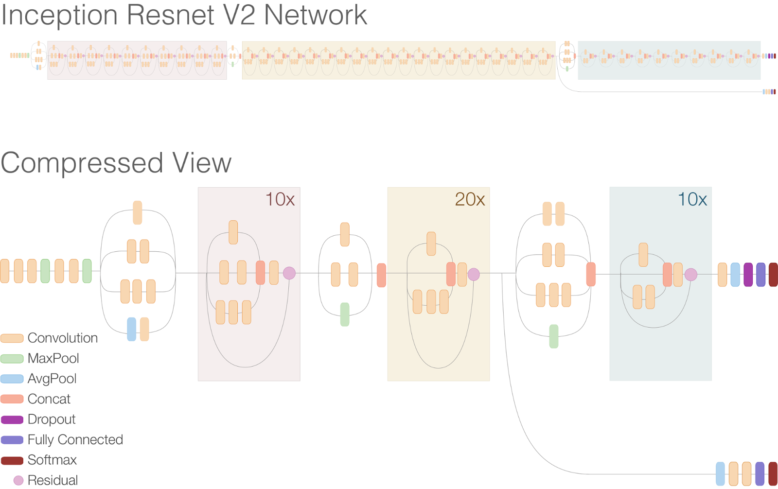
Our 2014 system used the Inception V1 image classification model to initialize the image encoder, which produces the encodings that are useful for recognizing different objects in the images. This was the best image model available at the time, achieving 89.6% top-5 accuracy on the benchmark ImageNet 2012 image classification task. We replaced this in 2015 with the newer Inception V2 image classification model, which achieves 91.8% accuracy on the same task. The improved vision component gave our captioning system an accuracy boost of 2 points in the BLEU-4 metric (which is commonly used in machine translation to evaluate the quality of generated sentences) and was an important factor of its success in the captioning challenge.

Today’s code release initializes the image encoder using the Inception V3 model, which achieves 93.9% accuracy on the ImageNet classification task. Initializing the image encoder with a better vision model gives the image captioning system a better ability to recognize different objects in the images, allowing it to generate more detailed and accurate descriptions. This gives an additional 2 points of improvement in the BLEU-4 metric over the system used in the captioning challenge.

Another key improvement to the vision component comes from fine-tuning the image model. This step addresses the problem that the image encoder is initialized by a model trained to classify objects in images, whereas the goal of the captioning system is to describe the objects in images using the encodings produced by the image model. For example, an image classification model will tell you that a dog, grass and a frisbee are in the image, but a natural description should also tell you the color of the grass and how the dog relates to the frisbee.

In the fine-tuning phase, the captioning system is improved by jointly training its vision and language components on human generated captions. This allows the captioning system to transfer information from the image that is specifically useful for generating descriptive captions, but which was not necessary for classifying objects. In particular, after fine-tuning it becomes better at correctly describing the colors of objects. Importantly, the fine-tuning phase must occur after the language component has already learned to generate captions - otherwise, the noisiness of the randomly initialized language component causes irreversible corruption to the vision component. For more details, read the full paper here.
Left: the better image model allows the captioning model to generate more detailed and accurate descriptions. Right: after fine-tuning the image model, the image captioning system is more likely to describe the colors of objects correctly.
Until recently our image captioning system was implemented in the DistBelief software framework. The TensorFlow implementation released today achieves the same level of accuracy with significantly faster performance: time per training step is just 0.7 seconds in TensorFlow compared to 3 seconds in DistBelief on an Nvidia K20 GPU, meaning that total training time is just 25% of the time previously required.

A natural question is whether our captioning system can generate novel descriptions of previously unseen contexts and interactions. The system is trained by showing it hundreds of thousands of images that were captioned manually by humans, and it often re-uses human captions when presented with scenes similar to what it’s seen before.
When the model is presented with scenes similar to what it’s seen before, it will often re-use human generated captions.
So does it really understand the objects and their interactions in each image? Or does it always regurgitate descriptions from the training data? Excitingly, our model does indeed develop the ability to generate accurate new captions when presented with completely new scenes, indicating a deeper understanding of the objects and context in the images. Moreover, it learns how to express that knowledge in natural-sounding English phrases despite receiving no additional language training other than reading the human captions.
Our model generates a completely new caption using concepts learned from similar scenes in the training set.
We hope that sharing this model in TensorFlow will help push forward image captioning research and applications, and will also allow interested people to learn and have fun. To get started training your own image captioning system, and for more details on the neural network architecture, navigate to the model’s home-page here. While our system uses the Inception V3 image classification model, you could even try training our system with the recently released Inception-ResNet-v2 model to see if it can do even better!

The 280-Year-Old Algorithm Inside Google Trips


Algorithms Engineering is a lot of fun because algorithms do not go out of fashion: one never knows when an oldie-but-goodie might come in handy. Case in point: Yesterday, Google announced Google Trips, a new app to assist you in your travels by helping you create your own “perfect day” in a city. Surprisingly, deep inside Google Trips, there is an algorithm that was invented 280 years ago.

In 1736, Leonhard Euler authored a brief but beautiful mathematical paper regarding the town of Königsberg and its 7 bridges, shown here:
Image from Wikipedia
In the paper, Euler studied the following question: is it possible to walk through the city crossing each bridge exactly once? As it turns out, for the city of Königsberg, the answer is no. To reach this answer, Euler developed a general approach to represent any layout of landmasses and bridges in terms of what he dubbed the Geometriam Situs (the “Geometry of Place”), which we now call Graph Theory. He represented each landmass as a “node” in the graph, and each bridge as an “edge,” like this:
Image from Wikipedia
Euler noticed that if all the nodes in the graph have an even number of edges (such graphs are called “Eulerian” in his honor) then, and only then, a cycle can be found that visits every edge exactly once. Keep this in mind, as we’ll rely on this fact later in the post.

Our team in Google Research has been fascinated by the “Geometry of Place” for some time, and we started investigating a question related to Euler’s: rather than visiting just the bridges, how can we visit as many interesting places as possible during a particular trip? We call this the “itineraries” problem. Euler didn’t study it, but it is a well known topic in Optimization, where it is often called the “Orienteering” problem.

While Euler’s problem has an efficient and exact solution, the itineraries problem is not just hard to solve, it is hard to even approximately solve! The difficulty lies in the interplay between two conflicting goals: first, we should pick great places to visit, but second, we should pick them to allow a good itinerary: not too much travel time; don’t visit places when they’re closed; don’t visit too many museums, etc. Embedded in such problems is the challenge of finding efficient routes, often referred to as the Travelling Salesman Problem (TSP).

Algorithms for Travel Itineraries

Fortunately, the real world has a property called the “triangle inequality” that says adding an extra stop to a route never makes it shorter. When the underlying geometry satisfies the triangle inequality, the TSP can be approximately solved using another algorithm discovered by Christofides in 1976. This is an important part of our solution, and builds on Euler’s paper, so we’ll give a quick four-step rundown of how it works here:
  1. We start with all our destinations separate, and repeatedly connect together the closest two that aren’t yet connected. This doesn’t yet give us an itinerary, but it does connect all the destinations via a minimum spanning tree of the graph.
  2. We take all the destinations that have an odd number of connections in this tree (Euler proved there must be an even number of these), and carefully pair them up.
  3. Because all the destinations now have an even number of edges, we’ve created an Eulerian graph, so we create a route that crosses each edge exactly once.
  4. We now have a great route, but it might visit some places more than once. No problem, we find any double visits and simply bypass them, going directly from the predecessor to the successor.
Christofides gave an elegant proof that the resulting route is always close to the shortest possible. Here’s an example of the Christofides’ algorithm in action on a location graph with the nodes representing places and the edges with costs representing the travel time between the places.
Construction of an Eulerian Tour in a location graph
Armed with this efficient route-finding subroutine, we can now start building itineraries one step at a time. At each step, we estimate the benefit to the user of each possible new place to visit, and likewise estimate the cost using the Christofides algorithm. A user’s benefit can be derived from a host of natural factors such as the popularity of the place and how different the place is relative to places already visited on the tour. We then pick whichever new place has the best benefit per unit of extra cost (e.g., time needed to include the new place in the tour). Here’s an example of our algorithm actually building a route in London using the location graph shown above:
Itineraries in Google Trips

With our first good approximate solution to the itineraries problem in hand, we started working with our colleagues from the Google Trips team, and we realized we’d barely scratched the surface. For instance, even if we produce the absolute perfect itinerary, any particular user of the system will very reasonably say, “That’s great, but all my friends say I also need to visit this other place. Plus, I’m only around for the morning, and I don’t want to miss this place you listed in the afternoon. And I’ve already seen Big Ben twice.” So rather than just producing an itinerary once and calling it a perfect day, we needed a fast dynamic algorithm for itineraries that users can modify on the fly to suit their individual taste. And because many people have bad data connections while traveling, the solution had to be efficient enough to run disconnected on a phone.

Better Itineraries Through the Wisdom of Crowds

While the algorithmic aspects of the problem were highly challenging, we realized that producing high-quality itineraries was just as dependent on our understanding of the many possible stopping points on the itinerary. We had Google’s extensive travel database to identify the interesting places to visit, and we also had great data from Google’s existing systems about how to travel from any place to any other. But we didn’t have a good sense for how people typically move through this geometry of places.

For this, we turned to the wisdom of crowds. This type of wisdom is used by Google to estimate delays on highways, and to discover when restaurants are most busy. Here, we use the same techniques to learn about common visit sequences that we can stitch together into itineraries that feel good to our users. We combine Google's knowledge of when places are popular, with the directions between those places to gather an idea of what tourists like to do when travelling.

And the crowd has a lot more wisdom to offer in the future. For example, we noticed that visits to Buckingham Palace spike around 11:30 and stay a bit longer than at other times of the day. This seemed a little strange to us, but when we looked more closely, it turns out to be the time of the Changing of the Guard. We’re looking now at ways to incorporate this type of timing information into the itinerary selection algorithms.

So give it a try: Google Trips, available now on Android and iOS, has you covered from departure to return.

The 2016 Google Earth Engine User Summit: Turning pixels into insights


"We are trying new methods [of flood modeling] in Earth Engine based on machine learning techniques which we think are cheaper, more scalable, and could exponentially drive down the cost of flood mapping and make it accessible to everyone."
-Beth Tellman, Arizona State University and Cloud to Street

Recently, Google headquarters hosted the Google Earth Engine User Summit 2016, a three-day hands-on technical workshop for scientists and students interested in using Google Earth Engine for planetary-scale cloud-based geospatial analysis. Earth Engine combines a multi-petabyte catalog of satellite imagery and geospatial datasets with a simple, yet powerful API backed by Google's cloud, which scientists and researchers use to detect, measure, and predict changes to the Earth's surface.
Earth Engine founder Rebecca Moore kicking off the first day of the summit
Summit attendees could choose among twenty-five hands-on workshops over the course of the three day summit, most generated for the summit specifically, giving attendees an exclusive introduction to the latest features in our platform. The sessions covered a wide range of topics and Earth Engine experience levels, from image classifiers and classifications, time series analysis, building custom web applications, all the way to arrays, matrices, and linear algebra in Earth Engine.
Terra Bella Product Manager, Kristi Bohl, taught a session on using SkySat imagery, like the image above over Sydney, Australia, for change detection. Workshop attendees also learned how to take advantage of the deep temporal stack the SkySat archive offers for change-over-time analyses.
Cross-correlation between Landsat 8 NDVI and the sum of CHIRPS precipitation. Red is high cross-correlation and blue is low. The gap in data is because CHIRPS is masked over water.
Nick Clinton, a developer advocate for Earth Engine, taught a time series session that covered statistical techniques as applied to satellite imagery data. Students learned how to make graphics like the above, which shows the cross-correlation between Landsat 8 NDVI and the sum of CHIRPS precipitation from the previous month over San Francisco, CA. The correlation should be high for relatively r-selected plants like grasses and weeds and relatively low for perennials, shrubs, or forest.

My workshop session covered how users can upload their own data into Earth Engine and the many different ways to take the results of their analyses with them, including rendering static map tiles hosted on Google Cloud Storage, exporting images, creating new assets, and even making movies, like this timelapse video of all the Sentinel 2A images captured over Sydney Australia.
Along with the workshop sessions, we hosted five plenary speakers and 18 lightning talk presenters. These presenters shared how Earth Engine fits into their research, spanning from drought monitoring, agriculture, conservation, flood risk mapping, and hydrological analysis.

Plenary Speakers
Lightning Presentations
Keeping our users first

It is always inspiring to see such a diverse group of people come together to celebrate, learn, and share all the amazing and wondrous things people are doing with Earth Engine. It is not only an opportunity for our users to learn the latest techniques; it is also a way for the Earth Engine team to experience the new and exciting ways people are harnessing Earth Engine to solve some of the most pressing environmental issues facing humanity.
We've already begun planning for next year's user summit, and based on the success of this year's, we're hoping to hold an even larger one.

Research from VLDB 2016: Improved Friend Suggestion using Ego-Net Analysis


On September 5 - 9, New Delhi, India hosted the 42nd International Conference on Very Large Data Bases (VLDB), a premier annual forum for academic and industry research on databases, data management, data mining and data analytics. Over the past several years, Google has actively participated in VLDB, both as official sponsor and with numerous contributions to the research and industrial tracks. In this post, we would like to share the research presented in one of the Google papers from VLDB 2016.

In Ego-net Community Mining Applied to Friend Suggestion, co-authored by Googlers Silvio Lattanzi, Vahab Mirrokni, Ismail Oner Sebe, Ahmed Taei, Sunita Verma and myself, we explore how social networks can provide better friend suggestions to users, a challenging practical problem faced by all social network platforms

Friend suggestion – the task of suggesting to a user the contacts she might already know in the network but that she hasn’t added yet – is major driver of user engagement and social connection in all online social networks. Designing a high quality system that can provide relevant and useful friend recommendations is very challenging, and requires state-of-the-art machine learning algorithms based on a multitude of parameters.

An effective family of features for friend suggestion consist of graph features such as the number of common friends between two users. While widely used, the number of common friends has some major drawbacks, including the following which is shown in Figure 1.
Figure 1: Ego-net of Sally.
In this figure we represent the social connections of Sally and her friends – the ego-net of Sally. An ego-net of a node (in this case, Sally) is defined as the graph that contains the node itself, all of the node’s neighbors and the connection among those nodes. Sally has 6 friends in her ego-net: Albert (her husband), Brian (her son), Charlotte (her mother) as well as Uma (her boss), Vincent and Wally (two of her team members). Notice how A, B and C are all connected with each other while they do not know U, V or W. On the other hand U, V and W have all added each other as their friend (except U and W who are good friend but somehow forgot to add each other).

Notice how each of A, B, C have a common friend with each of U, V and W: Sally herself. A friend recommendation system based on common neighbors might suggest to Sally’s son (for instance) to add Sally’s boss as his friend! In reality the situation is even more complicated because users’ online and offline friends span several different social circles or communities (family, work, school, sports, etc).

In our paper we introduce a novel technique for friend suggestions based on independently analyzing the ego-net structure. The main contribution of the paper is to show that it is possible to provide friend suggestions efficiently by constructing all ego-nets of the nodes in the graph and then independently applying community detection algorithms on them in large-scale distributed systems.

Specifically, the algorithm proceeds by constructing the ego-nets of all nodes and applying, independently on each of them, a community detection algorithm. More precisely the algorithm operates on so-called “ego-net-minus-ego” graphs, which is defined as the graph including only the neighbors of a given node, as shown in the figure below.
Figure 2: Clustering of the ego-net of Sally.
Notice how in this example the ego-net-minus-ego of Sally has two very clear communities: her family (A, B, C) and her co-workers (U, V, W) which are easily separated. Intuitively, this is because one might expect that while nodes (e.g. Sally) participate in many communities, there is usually a single (or a limited number of) contexts in which two specific neighbors interact. While Sally is both part of her family and work community, Sally and Uma interact only at work. Through extensive experimental evaluation on large-scale public social networks and formally through a simple mathematical model, our paper confirms this intuition. It seems that while communities are hard to separate in a global graph, they are easier to identify at the local level of ego-nets.

This allows for a novel graph-based method for friend suggestion which intuitively only allows suggestion of pairs of users that are clustered together in the same community from the point of view of their common friends. With this method, U and W will be suggested to add each other (as they are in the same community and they are not yet connected) while B and U will not be suggested as friends as they span two different communities.

From an algorithmic point of view, the paper introduces efficient parallel and distributed techniques for computing and clustering all ego-nets of very large graphs at the same time – a fundamental aspect enabling use of the system on the entire world Google+ graph. We have applied this feature in the “You May Know” system of Google+, resulting in a clear positive impact on the prediction task, improving the acceptance rate by more than 1.5% and decreasing the rejection rate by more than 3.3% (a significative impact at Google scales).

We believe that many future directions of work might stem from our preliminary results. For instance ego-net analysis could be potentially to automatically classify a user contacts in circles and to detect spam. Another interesting direction is the study of ego-network evolution in dynamic graphs.

Computational Thinking from a Dispositions Perspective


(Cross-posted on the Google for Education Blog)

In K–12 computer science (CS) education, much of the discussion about what students need to learn and do to has centered around computational thinking (CT). While much of the current work in CT education is focused on core concepts and their application, the one area of CT that has not been well explored is the relationship between CT as a problem solving model, and the dispositions or habits of mind that it can build in students of all ages.

Exploring the mindset that CT education can engender depends, in part, on the definition of CT itself. While there are a number of definitions of CT in circulation, Valerie Barr and I defined it in the following way:
CT is an approach to solving problems in a way that can be implemented with a computer. Students become not merely tool users but tool builders. They use a set of concepts, such as abstraction, recursion, and iteration, to process and analyze data, and to create real and virtual artifacts. CT is a problem solving methodology that can be automated and transferred and applied across subjects.
Like many others, our view of CT also included the core CT concepts: abstraction, algorithms and procedures, automation, data collection and analysis, data representation, modeling and simulation, parallelization and problem decomposition.
The idea of dispositions, however, comes from the field of vocational education and research on career development which focuses on the personal qualities or soft skills needed for employment (see full report from Economist Intelligence Unit here). These skills traditionally include being responsible, adaptable, flexible, self-directed, and self-motivated; being able to solve simple and complex problems, having integrity, self-confidence, and self-control. They can also include the ability to work with people of different ages and cultures, collaboration, complex communication and expert thinking.

Cuoco, Goldenberg, and Mark’s research also provided examples of what students should learn to develop the habits of mind used by scientists across numerous disciplines. These are: recognizing patterns, experimenting, describing, tinkering, inventing, visualizing, and conjecturing. Potter and Vickers also found that in the burgeoning field of cyber security “there is significant overlap between the roles for many soft skills, including analysis, consulting and process skills, leadership, and relationship management. Both communication and presentation skills were valued.”
CT, because of its emphasis on problem solving, provides a natural environment for embedding the idea of dispositions into K-12. According to the International Society for Technology in Education and the Computer Science Teachers Association, the set of dispositions that student practice and internalize while learning about CT can include:
  • confidence in dealing with complexity,
  • persistence in working with difficult problems,
  • the ability to handle ambiguity,
  • the ability to deal with open-ended problems,
  • setting aside differences to work with others to achieve a common goal or solution, and
  • knowing one's strengths and weaknesses when working with others.
Any teacher in any discipline is likely to tell you that persistence, problem solving, collaboration and awareness of one’s strengths and limitations are critical to successful learning for all students. So how do we make these dispositions a more explicit part of the CT curriculum? One of the ways to do so is to to call them out directly to students and explain why they are important in all areas of their study, career, and lives. In addition educators can:
  • Post in the classroom­­ a list of the Dispositions Leading to Success,
  • Help familiarize students with these dispositions by using the terms when talking with students and referring to the work they are doing. “Today we are going to be solving an open-ended problem. What do you think that means?”
  • Help students understand that they are developing these dispositions by congratulating them when these dispositions lead to success: “Great problem-solving skills!”; “Great job! Your persistence helped solve the problem”; “You dealt with ambiguity really well!”.
  • Engage students in discussions about the dispositions: “Today we are going to work in teams. What does it mean to be on a team? What types of people would you want on your team and why?”
  • Help students articulate their dispositions when developing their resumes or preparing for job interviews.
Guest speakers from industry might also:
  • Integrate the importance of dispositions into their talks with students: examples of the problems they have solved, how the different skills of team members led to different solutions, the role persistence played in solving a problem/developing a product or service…
  • Talk about the importance of dispositions to employers and how they contribute to their own organizational culture, the ways employers ask interviewees about their dispositions or how interviewees might respond (e.g. use the terms and give examples).
As Google’s Director of Education and University Relations, Maggie Johnson noted in a recent blog post, CT represents a core set of skills that are necessary for all students:
If we can make these explicit connections for students, they will see how the devices and apps that they use everyday are powered by algorithms and programs. They will learn the importance of data in making decisions. They will learn skills that will prepare them for a workforce that will be doing vastly different tasks than the workforce of today.
In addition to these concepts, we can now add developing critical dispositions for success in computing and in life to the list of benefits for teaching CT to all students.

Announcing the First Annual Global PhD Fellowship Summit and the 2016 Google PhD Fellows


In 2009, Google created the PhD Fellowship Program to recognize and support outstanding graduate students doing exceptional research in Computer Science and related disciplines. Now in its eighth year, our Fellowships have helped support over 250 graduate students in Australia, China and East Asia, India, North America, Europe and the Middle East who seek to shape and influence the future of technology.

Recently, Google PhD Fellows from around the globe converged on our Mountain View campus for the first annual Global PhD Fellowship Summit. The students heard talks from researchers like Jeff Dean, Françoise Beaufays, Peter Norvig, Maya Gupta and Amin Vahdat, and got a glimpse into some of the state-of-the-art research pursued across Google.
Senior Google Fellow Jeff Dean shares how TensorFlow is used at Google
Fellows also had the chance to connect one-on-one with Googlers to discuss their research, as well as receive feedback from leaders in their fields. The event wrapped up with a panel discussion with Dan Russell, Kristen LeFevre, Douglas Eck and Françoise Beaufays about their unique career paths. Maggie Johnson concluded the Summit by sharing about the different types of research environments across academia and industry.
(Left) PhD Fellows share their work with Google researchers during the poster session
(Right) Research panelists share their journeys through academia and industry
Our PhD Fellows represent some the best and brightest young researchers around the globe in Computer Science and it is our ongoing goal to support them as they make their mark on the world.

We’d also like to welcome the newest class of Google PhD Fellows recently awarded in China and East Asia, India, and Australia. We look forward to seeing each of them at next year’s summit!

2016 Global PhD Fellows

Computational Neuroscience
Cameron (Po-Hsuan) Chen, Princeton University
Grace Lindsay, Columbia University
Martino Sorbaro Sindaci, The University of Edinburgh

Human-Computer Interaction
Dana McKay, University of Melbourne
Koki Nagano, University of Southern California
Arvind Satyanarayan, Stanford University
Amy Xian Zhang, Massachusetts Institute of Technology

Machine Learning
Olivier Bachem, Swiss Federal Institute of Technology Zurich
Tianqi Chen, University of Washington
Emily Denton, New York University
Kwan Hui Lim, University of Melbourne
Yves-Laurent Kom Samo, University of Oxford
Woosang Lim, Korea Advanced Institute of Science and Technology
Anirban Santara, Indian Institute of Technology Kharagpur
Daniel Jaymin Mankowitz, Technion - Israel Institute of Technology
Lucas Maystre, École Polytechnique Fédérale de Lausanne
Arvind Neelakantan, University of Massachusetts, Amherst
Ludwig Schmidt, Massachusetts Institute of Technology
Quanming Yao, The Hong Kong University of Science and Technology
Shandian Zhe, Purdue University, West Lafayette

Machine Perception, Speech Technology and Computer Vision
Eugen Beck, RWTH Aachen University
Yu-Wei Chao, University of Michigan, Ann Arbor
Wei Liu, University of North Carolina at Chapel Hill
Aron Monszpart, University College London
Thomas Schoeps, Swiss Federal Institute of Technology Zurich
Tian Tan, Shanghai Jiao Tong University
Chia-Yin Tsai, Carnegie Mellon University
Weitao Xu, University of Queensland

Market Algorithms
Hossein Esfandiari, University of Maryland, College Park
Sandy Heydrich, Saarland University - Saarbrucken GSCS
Rad Niazadeh, Cornell University
Sadra Yazdanbod, Georgia Institute of Technology

Mobile Computing
Lei Kang, University of Wisconsin
Tauhidur Rahman, Cornell University
Chungkuk Yoo, Korea Advanced Institute of Science and Technology
Yuhao Zhu, University of Texas, Austin

Natural Language Processing
Tamer Alkhouli, RWTH Aachen University
Jose Camacho Collados, Sapienza - Università di Roma

Privacy and Security
Chitra Javali, University of New South Wales
Kartik Nayak, University of Maryland, College Park
Nicolas Papernot, Pennsylvania State University
Damian Vizar, École Polytechnique Fédérale de Lausanne
Xi Wu, University of Wisconsin

Programming Languages, Algorithms and Software Engineering
Marcelo Sousa, University of Oxford
Arpita Biswas, Indian Institute of Science

Structured Data and Database Management
Xiang Ren, University of Illinois, Urbana-Champaign

Systems and Networking
Ying Chen, Tsinghua University
Andrew Crotty, Brown University
Aniruddha Singh Kushwaha, Indian Institute of Technology Bombay
Ilias Marinos, University of Cambridge
Kay Ousterhout, University of California, Berkeley
Hong Zhang, The Hong Kong University of Science and Technology

Reproducible Science: Cancer Researchers Embrace Containers in the Cloud


Today we hear from the principal investigators of the ICGC-TCGA DREAM Somatic Mutation Calling Challenges about how they are encouraging cancer researchers to make use of Docker and Google Cloud Platform to gain a deeper understanding of the complex genetic mutations that occur in cancer, while doing so in a reproducible way.
– Nicole Deflaux and Jonathan Bingham, Google Genomics

Today’s genomic analysis software tools often give different answers when run in different computing environments - that’s like getting a different diagnosis from your doctor depending on which examination room you’re sitting in. Reproducible science matters, especially in cancer research where so many lives are at stake. The Cancer Moonshot has called for the research world to 'Break down silos and bring all the cancer fighters together'. Portable software “containers” and cloud computing hold the potential to help achieve these goals by making scientific data analysis more reproducible, reusable and scalable.

Our team of researchers from the Ontario Institute for Cancer Research, University of California Santa Cruz, Sage Bionetworks and Oregon Health and Sciences University is pushing the frontiers by encouraging scientists to package up their software in reusable Docker containers and make use of cloud-resident data from the Cancer Cloud Pilots funded by the National Cancer Institute.

In 2014 we initiated the ICGC-TCGA DREAM Somatic Mutation Calling (SMC) Challenges where Google provided credits on Google Cloud Platform. The first result of this collaboration was the DREAM-SMC DNA challenge, a public challenge that engaged cancer researchers from around the world to find the best methods for discovering DNA somatic mutations. By the end of the challenge, over 400 registered participants competed by submitting 3,500 open-source entries for 14 test genomes, providing key insights on the strengths and limitations of the current mutation detection methods.

The SMC-DNA challenge enabled comparison of results, but it did little to facilitate the exchange of cross-platform software tools. Accessing extremely large genome sequence input files and shepherding complex software pipelines created a “double whammy” to discourage data sharing and software reuse.

How can we overcome these barriers?

Exciting developments have taken place in the past couple of years that may annihilate these last barriers. The availability of cloud technologies and containerization can serve as the vanguards of reproducibility and interoperability.

Thus, a new way of creating open DREAM challenges has emerged: rather than encouraging the status quo where participants run their own methods themselves on their own systems, and the results cannot be verified, the new challenge design requires participants to submit open-source code packaged in Docker containers so that anyone can run their methods and verify the results. Real-time leaderboards show which entries are winning and top performers have a chance to claim a prize.

Working with Google Genomics and Google Cloud Platform, the DREAM-SMC organizers are now using cloud and containerization technologies to enable portability and reproducibility as a core part of the DREAM challenges. The latest SMC installments, the SMC-Het Challenge and the SMC-RNA Challenge have implemented this new plan:

  • SMC-Het Challenge: Tumour biopsies are composed of many different cell types in addition to tumour cells, including normal tissue and infiltrating immune cells. Furthermore, the tumours themselves are made of a mixture of different subpopulations, all related to one another through cell division and mutation. Critically, each sub-population can have distinct clinical outcomes, with some more resistant to treatment or more likely to metastasize than others. The goal of the SMC-Het Challenge is to identify the best methods for predicting tumor subpopulations and their “family tree” of relatedness from genome sequencing data.
  • SMC-RNA Challenge: The alteration of RNA production is a fundamental mechanism by which cancer cells rewire cellular circuitry. Genomic rearrangements in cancer cells can produce fused protein products that can bestow Frankenstein-like properties. Both RNA abundances and novel fusions can serve as the basis for clinically-important prognostic biomarkers. The SMC-RNA Challenge will identify the best methods to detect such rogue expressed RNAs in cancer cells.

Ultimately, the success will be gauged by the amount of serious participation in these latest competitions. So far, the signs are encouraging. SMC-Het, which focuses on a very new research area, launched in November 2015 and has already enlisted 18 teams contributing over 70 submissions. SMC-RNA just recently launched and will run until early 2017, with several of the world leaders in the field starting to prepare entries. What’s great about the submissions being packaged in containers is that even after the challenges end, the tested methods can be applied and further adapted by anyone around the world.

Thus, the moon shot need not be a lucky solo attempt made by one hero in one moment of inspiration. Instead, the new informatics of clouds and containers will enable us to combine intelligence so we can build a series of bridges from here to there.

To participate in the DREAM challenges, visit the SMC-Het and SMC-RNA Challenge sites.

Improving Inception and Image Classification in TensorFlow


Earlier this week, we announced the latest release of the TF-Slim library for TensorFlow, a lightweight package for defining, training and evaluating models, as well as checkpoints and model definitions for several competitive networks in the field of image classification.

In order to spur even further progress in the field, today we are happy to announce the release of Inception-ResNet-v2, a convolutional neural network (CNN) that achieves a new state of the art in terms of accuracy on the ILSVRC image classification benchmark. Inception-ResNet-v2 is a variation of our earlier Inception V3 model which borrows some ideas from Microsoft's ResNet papers [1][2]. The full details of the model are in our arXiv preprint Inception-v4, Inception-ResNet and the Impact of Residual Connections on Learning.

Residual connections allow shortcuts in the model and have allowed researchers to successfully train even deeper neural networks, which have lead to even better performance. This has also enabled significant simplification of the Inception blocks. Just compare the model architectures in the figures below:
Schematic diagram of Inception V3
Schematic diagram of Inception-ResNet-v2
At the top of the second Inception-ResNet-v2 figure, you'll see the full network expanded. Notice that this network is considerably deeper than the previous Inception V3. Below in the main figure is an easier to read version of the same network where the repeated residual blocks have been compressed. Here, notice that the inception blocks have been simplified, containing fewer parallel towers than the previous Inception V3.

The Inception-ResNet-v2 architecture is more accurate than previous state of the art models, as shown in the table below, which reports the Top-1 and Top-5 validation accuracies on the ILSVRC 2012 image classification benchmark based on a single crop of the image. Furthermore, this new model only requires roughly twice the memory and computation compared to Inception V3.


Model
Architecture

Checkpoint

Top-1 Accuracy

Top-5 Accuracy

Code
80.4
95.3

Code
78.0
93.9

Code
76.8
93.2

Code
TBA
79.9*
95.2*
(*): Results quoted in ResNet paper.

As an example, while both Inception V3 and Inception-ResNet-v2 models excel at identifying individual dog breeds, the new model does noticeably better. For instance, whereas the old model mistakenly reported Alaskan Malamute for the picture on the right, the new Inception-ResNet-v2 model correctly identifies the dog breeds in both images.
An Alaskan Malamute (left) and a Siberian Husky (right). Images from Wikipedia
In order to allow people to immediately begin experimenting, we are also releasing a pre-trained instance of the new Inception-ResNet-v2, as part of the TF-Slim Image Model Library.

We are excited to see what the community does with this improved model, following along as people adapt it and compare its performance on various tasks. Want to get started? See the accompanying instructions on how to train, evaluate or fine-tune a network.

As always, releasing the code was a team effort. Specific thanks are due to:
  • Model Architecture - Christian Szegedy, Sergey Ioffe, Vincent Vanhoucke, Alex Alemi
  • Systems Infrastructure - Jon Shlens, Benoit Steiner, Mark Sandler, and David Andersen
  • TensorFlow-Slim - Sergio Guadarrama and Nathan Silberman
  • Model Visualization - Fernanda Viégas and James Wexler

TF-Slim: A high level library to define complex models in TensorFlow


Earlier this year, we released a TensorFlow implementation of a state-of-the-art image classification model known as Inception-V3. This code allowed users to train the model on the ImageNet classification dataset via synchronized gradient descent, using either a single local machine or a cluster of machines. The Inception-V3 model was built on an experimental TensorFlow library called TF-Slim, a lightweight package for defining, training and evaluating models in TensorFlow. The TF-Slim library provides common abstractions which enable users to define models quickly and concisely, while keeping the model architecture transparent and its hyperparameters explicit.

Since that release, TF-Slim has grown substantially, with many types of layers, loss functions, and evaluation metrics added, along with handy routines for training and evaluating models. These routines take care of all the details you need to worry about when working at scale, such as reading data in parallel, deploying models on multiple machines, and more. Additionally, we have created the TF-Slim Image Models library, which provides definitions and training scripts for many widely used image classification models, using standard datasets. TF-Slim and its components are already widely used within Google, and many of these improvements have already been integrated into tf.contrib.slim.

Today, we are proud to share the latest release of TF-Slim with the TF community. Some highlights of this release include:
Want to get started using TF-Slim? See the README for details. Interested in working with image classification models? See these instructions or this Jupyter notebook.

The release of the TF-Slim library and the pre-trained model zoo has been the result of widespread collaboration within Google Research. In particular we want to highlight the vital contributions of the following researchers:
  • TF-Slim: Sergio Guadarrama, Nathan Silberman.
  • Model Definitions and Checkpoints: Christian Szegedy, Sergey Ioffe, Vincent Vanhoucke, Jon Shlens, Zbigniew Wojna, Vivek Rathod, George Papandreou, Alex Alemi
  • Systems Infrastructure: Jon Shlens, Matthieu Devin, Martin Wicke
  • Jupyter notebook: Nathan Silberman, Kevin Murphy
References:
[1] Going deeper with convolutions, Christian Szegedy, Wei Liu, Yangqing Jia, Pierre Sermanet, Scott Reed, Dragomir Anguelov, Dumitru Erhan, Vincent Vanhoucke, Andrew Rabinovich, CVPR 2015
[2] Batch Normalization: Accelerating Deep Network Training by Reducing Internal Covariate Shift Sergey Ioffe, Christian Szegedy, ICML 2015
[3] Rethinking the Inception Architecture for Computer Vision, Christian Szegedy, Vincent Vanhoucke, Sergey Ioffe, Jonathon Shlens, Zbigniew Wojna, arXiv technical report 2015
[4] Very Deep Convolutional Networks for Large-Scale Image Recognition, Karen Simonyan, Andrew Zisserman, ICLR 2015
[5] ImageNet Classification with Deep Convolutional Neural Networks, Alex Krizhevsky, Ilya Sutskever, Geoffrey E. Hinton, NIPS 2012
[6] Deep Residual Learning for Image Recognition, Kaiming He, Xiangyu Zhang, Shaoqing Ren, Jian Sun, CVPR 2016

Text summarization with TensorFlow


Every day, people rely on a wide variety of sources to stay informed -- from news stories to social media posts to search results. Being able to develop Machine Learning models that can automatically deliver accurate summaries of longer text can be useful for digesting such large amounts of information in a compressed form, and is a long-term goal of the Google Brain team.

Summarization can also serve as an interesting reading comprehension test for machines. To summarize well, machine learning models need to be able to comprehend documents and distill the important information, tasks which are highly challenging for computers, especially as the lengths of the documents increases.

In an effort to push this research forward, we’re open-sourcing TensorFlow model code for the task of generating news headlines on Annotated English Gigaword, a dataset often used in summarization research. We also specify the hyper-parameters in the documentation that achieve better than published state-of-the-art on the most commonly used metric as of the time of writing. Below we also provide samples generated by the model.

Extractive and Abstractive summarization

One approach to summarization is to extract parts of the document that are deemed interesting by some metric (for example, inverse-document frequency) and join them to form a summary. Algorithms of this flavor are called extractive summarization.
Original Text: Alice and Bob took the train to visit the zoo. They saw a baby giraffe, a lion, and a flock of colorful tropical birds. 
Extractive Summary: Alice and Bob visit the zoo. saw a flock of birds.
Above we extract the words bolded in the original text and concatenate them to form a summary. As we can see, sometimes the extractive constraint can make the summary awkward or grammatically strange.

Another approach is to simply summarize as humans do, which is to not impose the extractive constraint and allow for rephrasings. This is called abstractive summarization.
Abstractive summary: Alice and Bob visited the zoo and saw animals and birds.
In this example, we used words not in the original text, maintaining more of the information in a similar amount of words. It’s clear we would prefer good abstractive summarizations, but how could an algorithm begin to do this?

About the TensorFlow model

It turns out for shorter texts, summarization can be learned end-to-end with a deep learning technique called sequence-to-sequence learning, similar to what makes Smart Reply for Inbox possible. In particular, we’re able to train such models to produce very good headlines for news articles. In this case, the model reads the article text and writes a suitable headline.

To get an idea of what the model produces, you can take a look at some examples below. The first column shows the first sentence of a news article which is the model input, and the second column shows what headline the model has written.

Input: Article 1st sentence
Model-written headline
metro-goldwyn-mayer reported a third-quarter net loss of dlrs 16 million due mainly to the effect of accounting rules adopted this year
mgm reports 16 million net loss on higher revenue
starting from july 1, the island province of hainan in southern china will implement strict market access control on all incoming livestock and animal products to prevent the possible spread of epidemic diseases
hainan to curb spread of diseases
australian wine exports hit a record 52.1 million liters worth 260 million dollars (143 million us) in september, the government statistics office reported on monday
australian wine exports hit record high in september

Future Research

We’ve observed that due to the nature of news headlines, the model can generate good headlines from reading just a few sentences from the beginning of the article. Although this task serves as a nice proof-of-concept, we started looking at more difficult datasets where reading the entire document is necessary to produce good summaries. In those tasks training from scratch with this model architecture does not do as well as some other techniques we’re researching, but it serves as a baseline. We hope this release can also serve as a baseline for others in their summarization research.