Author Archives: Google AI

FedJAX: Federated Learning Simulation with JAX

Federated learning is a machine learning setting where many clients (i.e., mobile devices or whole organizations, depending on the task at hand) collaboratively train a model under the orchestration of a central server, while keeping the training data decentralized. For example, federated learning makes it possible to train virtual keyboard language models based on user data that never leaves a mobile device.

Federated learning algorithms accomplish this by first initializing the model at the server and completing three key steps for each round of training:

  1. The server sends the model to a set of sampled clients.
  2. These sampled clients train the model on local data.
  3. After training, the clients send the updated models to the server and the server aggregates them together.
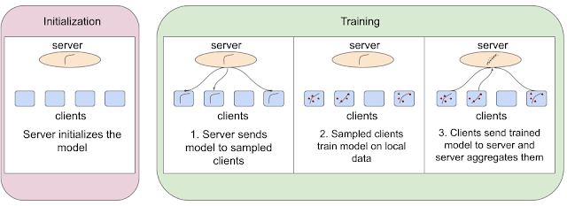
An example federated learning algorithm with four clients.

Federated learning has become a particularly active area of research due to an increased focus on privacy and security. Being able to easily translate ideas into code, iterate quickly, and compare and reproduce existing baselines is important for such a fast growing field.

In light of this, we are excited to introduce FedJAX, a JAX-based open source library for federated learning simulations that emphasizes ease-of-use in research. With its simple building blocks for implementing federated algorithms, prepackaged datasets, models and algorithms, and fast simulation speed, FedJAX aims to make developing and evaluating federated algorithms faster and easier for researchers. In this post we discuss the library structure and contents of FedJAX. We demonstrate that on TPUs FedJAX can be used to train models with federated averaging on the EMNIST dataset in a few minutes, and the Stack Overflow dataset in roughly an hour with standard hyperparameters.

Library Structure
Keeping ease of use in mind, FedJAX introduces only a few new concepts. Code written with FedJAX resembles the pseudo-code used to describe novel algorithms in academic papers, making it easy to get started. Additionally, while FedJAX provides building blocks for federated learning, users can replace these with the most basic implementations using just NumPy and JAX while still keeping the overall training reasonably fast.

Included Dataset and Models
In the current landscape of federated learning research, there are a variety of commonly used datasets and models, such as image recognition, language modeling, and more. A growing number of these datasets and models can be used straight out of the box in FedJAX, so the preprocessed datasets and models do not have to be written from scratch. This not only encourages valid comparisons between different federated algorithms but also accelerates the development of new algorithms.

At present, FedJAX comes packaged with the following datasets and sample models:

In addition to these standard setups, FedJAX provides tools to create new datasets and models that can be used with the rest of the library. Finally, FedJAX comes with standard implementations of federated averaging and other federated algorithms for training a shared model on decentralized examples, such as adaptive federated optimizers, agnostic federated averaging, and Mime, to make comparing and evaluating against existing algorithms easier.

Performance Evaluation
We benchmarked a standard FedJAX implementation of adaptive federated averaging on two tasks: the image recognition task for the federated EMNIST-62 dataset and the next word prediction task for the Stack Overflow dataset. Federated EMNIST-62 is a smaller dataset that consists of 3400 users and their writing samples, which are one of 62 characters (alphanumeric), while the Stack Overflow dataset is much larger and consists of millions of questions and answers from the Stack Overflow forum for hundreds of thousands of users.

We measured performance on various hardware specialized for machine learning. For federated EMNIST-62, we trained a model for 1500 rounds with 10 clients per round on GPU (NVIDIA V100) and TPU (1 TensorCore on a Google TPU v2) accelerators.

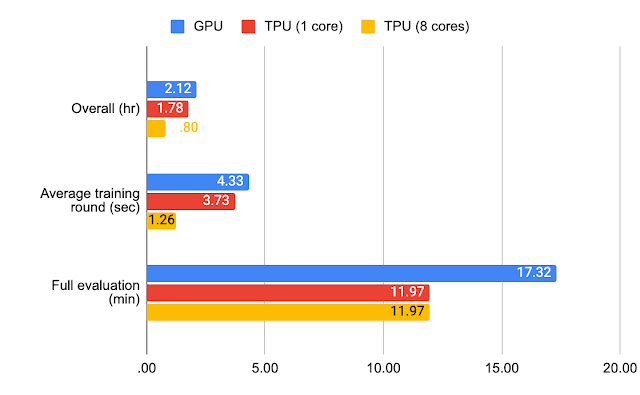
For Stack Overflow, we trained a model for 1500 rounds with 50 clients per round on GPU (NVIDIA V100) using jax.jit, TPU (1 TensorCore on a Google TPU v2) using only jax.jit, and multi-core TPU (8 TensorCores on a Google TPU v2) using jax.pmap. In the charts below, we’ve recorded the average training round completion time, time taken for full evaluation on test data, and time for the overall execution, which includes both training and full evaluation.
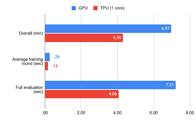
Benchmark results for federated EMNIST-62.
Benchmark results for Stack Overflow.

With standard hyperparameters and TPUs, the full experiments for federated EMNIST-62 can be completed in a few minutes and roughly an hour for Stack Overflow.
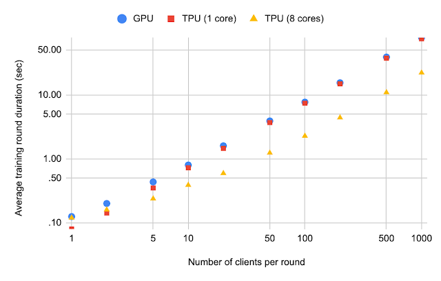
Stack Overflow average training round duration as the number of clients per round increases.

We also evaluate the Stack Overflow average training round duration as the number of clients per round increases. By comparing the average training round duration between TPU (8 cores) and TPU (1 core) in the figure, it is evident that using multiple TPU cores results in considerable runtime improvement if the number of clients participating per round is large (useful for applications like differentially private learning).

Conclusions and Future Work
In this post, we introduced FedJAX, a fast and easy-to-use federated learning simulation library for research. We hope that FedJAX will foster even more investigation and interest in federated learning. Moving forward, we plan to continually grow our existing collection of algorithms, aggregation mechanisms, datasets, and models.

Feel free to take a look at some of our tutorial notebooks, or try out FedJAX yourself! For more information about the library and relationship to platforms, such as Tensorflow Federated, see our paper, README, or FAQs.

Acknowledgements
We would like to thank Ke Wu and Sai Praneeth Kamireddy for contributing to the library and various discussions during development.

We would also like to thank Ehsan Amid, Theresa Breiner, Mingqing Chen, Fabio Costa, Roy Frostig, Zachary Garrett, Alex Ingerman, Satyen Kale, Rajiv Mathews, Lara Mcconnaughey, Brendan McMahan, Mehryar Mohri, Krzysztof Ostrowski, Max Rabinovich, Michael Riley, Vlad Schogol, Jane Shapiro, Gary Sivek, Luciana Toledo-Lopez, and Michael Wunder for helpful comments and contributions.

Source: Google AI Blog


Efficient Partitioning of Road Networks

Design techniques based on classical algorithms have proved useful for recent innovation on several large-scale problems, such as travel itineraries and routing challenges. For example, Dijkstra’s algorithm is often used to compute routes in graphs, but the size of the computation can increase quickly beyond the scale of a small town. The process of "partitioning" a road network, however, can greatly speed up algorithms by effectively shrinking how much of the graph is searched during computation.

In this post, we cover how we engineered a graph partitioning algorithm for road networks using ideas from classic algorithms, parts of which were presented in “Sketch-based Algorithms for Approximate Shortest Paths in Road Networks” at WWW 2021. Using random walks, a classical concept that is counterintuitively useful for computing shortest routes by decreasing the network size significantly, our algorithm can find a high quality partitioning of the whole road network of the North America continent nearly an order of magnitude faster1 than other partitioning algorithms with similar output qualities.

Using Graphs to Model Road Networks
There is a well-known and useful correspondence between road networks and graphs, where intersections become nodes and roads become edges.

Image from Wikipedia

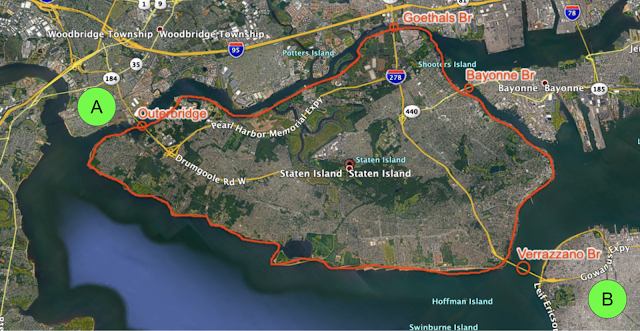
To understand how routing might benefit from partitioning, consider the most well-known solution for finding the fastest route: the Dijkstra algorithm, which works in a breadth-first search manner. The Dijkstra algorithm performs an exhaustive search starting from the source until it finds the destination. Because of this, as the distance between the source and the destination increases, the computation can become an order of magnitude slower. For example, it is faster to compute a route inside Seattle, WA than from Seattle, WA to San Francisco, CA. Moreover, even for intra-metro routes, the exhaustive volume of space explored by the Dijkstra algorithm during computation results in an impractical latency on the order of seconds. However, identifying regions that have more connections inside themselves, but fewer connections to the outside (such as Staten Island, NY) makes it possible to split the computation into multiple, smaller chunks.

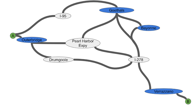
Top: A routing problem around Staten Island, NY. Bottom: Corresponding partitioning as a graph. Blue nodes indicate the only entrances to/exits from Staten Island.

Consider driving from point A to point B in the above image. Once one decides where to enter Staten Island (Outerbridge or Goethals) and where to exit (Verrazzano), the problem can be broken into the three smaller pieces of driving: To the entrance, the exit, and then the destination using the best route available. That means a routing algorithm only needs to consider these special points (beacons) to navigate between points A and B and can thus find the shortest accurate path faster.

Note that beacons are only useful as long as there are not too many of them—the fewer beacons there are, the fewer shortcuts need to be added, the smaller the search space, and the faster the computation—so a good partitioning should have relatively fewer beacons for the number of components (i.e., a particular area of a road network).

As the example of Staten Island illustrates, real-life road networks have many beacons (special points such as bridges, tunnels, or mountain passes) that result in some areas being very well-connected (e.g., with large grids of streets) and others being poorly connected (e.g., an island only accessible via a couple of bridges). The question becomes how to efficiently define the components and identify the smallest number of beacons that connect the road network.

Our Partitioning Algorithm
Because each connection between two components is a potential beacon, the approach we take to ensure there are not too many beacons is to divide the road network in a way that minimizes the number of connections between components.

To do this, we start by dividing the network into two balanced (i.e., of similar size) components while also minimizing the number of roads that connect those two components, which results in an effectively small ratio of beacons to roads in each component. Then, the algorithm keeps dividing the network into two at a time until all the components reach the desired size, in terms of the number of roads inside, that yields a useful multi-component partition. There is a careful balance here: If the size is too small, we will get too many beacons; whereas if it is too large, then it will be useful only for long routes. Therefore the size is left as an input parameter and found through experimentation when the algorithm is being finalized.

While there are numerous partitioning schemes, such as METIS (for general networks), PUNCH and inertial-flow (both optimized for road-network likes), our solution is based on the inertial-flow algorithm, augmented to run as efficiently on whole continents as it does on cities.

Balanced Partitioning for Road Networks
How does one divide a road network represented as a graph into two balanced components, as mentioned above? A first step is to make a graph smaller by grouping closely connected nodes together, which allows us to speed up the following two-way partitioning phase. This is where a random walk is useful.

Random walks enjoy many useful theoretical properties—which is why they have been used to study a range of topics from the motion of mosquitoes in a forest to heat diffusion—and that most relevant for our application is that they tend to get “trapped” in regions that are well connected inside but poorly connected outside. Consider a random walk on the streets of Staten Island for a fixed number of steps: because relatively few roads exit the island, most of the steps happen inside the island, and the probability of stepping outside the island is low.

Illustration of a random walk. Suppose the blue graph is a hypothetical road network corresponding to Staten Island. 50 random walks are performed, all starting at the middle point. Each random walk continues for 10 steps or until it steps out of the island. The numbers at each node depict how many times they were visited by a random walk. By the end, any node inside the island is visited much more frequently than the nodes outside.

After finding these small components, which will be highly connected nodes grouped together (such as Staten Island in the above example), the algorithm contracts each group into a new, single node.

Reducing the size of the original graph (left) by finding groups of nodes (middle) and coalescing each group into a single “super” node (right). Example here chosen manually to better illustrate the rest of the algorithm.

The final steps of the algorithm are to partition this much smaller graph into two parts and then refine the partitioning on this small graph to one on the original graph of the road network. We then use the inertial flow algorithm to find the cut on the smaller graph that minimizes the ratio of beacons (i.e., edges being cut) to nodes.

The algorithm evaluates different directions. For each direction, we find the division that minimizes the number of edges cut (e.g., beacons) between the first and last 10% of the nodes

Having found a cut on the small graph, the algorithm performs a refinement step to project the cut back to the original graph of the road network.

Conclusion
This work shows how classical algorithms offer many useful tools for solving problems at large scale. Graph partitioning can be used to break down a large scale graph problem into smaller subproblems to be solved independently and in parallel—which is particularly relevant in Google maps, where this partitioning algorithm is used to efficiently compute routes.

Acknowledgements
We thank our collaborators Lisa Fawcett, Sreenivas Gollapudi, Kostas Kollias, Ravi Kumar, Andrew Tomkins, Ameya Velingker from Google Research and Pablo Beltran, Geoff Hulten, Steve Jackson, Du Nguyen from Google Maps.


1This technique can also be used for any network structure, such as that for brain neurons. 

Source: Google AI Blog


Improving Generalization in Reinforcement Learning using Policy Similarity Embeddings

Reinforcement learning (RL) is a sequential decision-making paradigm for training intelligent agents to tackle complex tasks such as robotic locomotion, playing video games, flying stratospheric balloons and designing hardware chips. While RL agents have shown promising results in a variety of activities, it is difficult to transfer the capabilities of these agents to new tasks, even when these tasks are semantically equivalent. For example, consider a jumping task, where an agent, learning from image observations, needs to jump over an obstacle. Deep RL agents trained on a few of these tasks with varying obstacle positions struggle to successfully jump with obstacles at previously unseen locations.

Jumping task: The agent (white block), learning from pixels, needs to jump over an obstacle (gray square). The challenge is to generalize to unseen obstacle positions and floor heights in test tasks using a small number of training tasks. In a given task, the agent needs to time the jump precisely, at a specific distance from the obstacle, otherwise it will eventually hit the obstacle.

In “Contrastive Behavioral Similarity Embeddings for Generalization in Reinforcement Learning”, presented as a spotlight at ICLR 2021, we incorporate the inherent sequential structure in RL into the representation learning process to enhance generalization in unseen tasks. This is orthogonal to the predominant approaches before this work, which were typically adapted from supervised learning, and, as such, largely ignore this sequential aspect. Our approach exploits the fact that an agent, when operating in tasks with similar underlying mechanics, exhibits at least short sequences of behaviors that are similar across these tasks.

Prior work on generalization was typically adapted from supervised learning and revolved around enhancing the learning process. These approaches rarely exploit properties of the sequential aspect such as similarity in actions across temporal observations.

Our approach trains the agent to learn a representation in which states are close when the agent’s optimal behavior in these states and future states are similar. This notion of proximity, which we call behavioral similarity, generalizes to observations across different tasks. To measure behavioral similarity between states across various tasks (e.g., distinct obstacle positions in the jumping task), we introduce the policy similarity metric (PSM), a theoretically motivated state-similarity metric inspired by bisimulation. For example, the image below shows that the agent’s future actions in the two visually different states are the same, making these states similar according to PSM.

Understanding behavioral similarity. The agent (blue icon) needs to obtain the reward while maintaining distance from danger. Even though the initial states are visually different, they are similar in terms of their optimal behavior at current states as well as future states following the current state. Policy similarity metric (PSM) assigns high similarity to such behaviorally similar states and low similarity to dissimilar states.

For enhancing generalization, our approach learns state embeddings, which correspond to neural-network–based representations of task states, that bring together behaviorally similar states (such as in the figure above) while pushing behaviorally dissimilar states apart. To do so, we present contrastive metric embeddings (CMEs) that harness the benefits of contrastive learning for learning representations based on a state-similarity metric. We instantiate contrastive embeddings with the policy similarity metric (PSM) to learn policy similarity embeddings (PSEs). PSEs assign similar representations to states with similar behavior at both those states and future states, such as the two initial states shown in the image above.

As shown in the results below, PSEs considerably enhance generalization on the jumping task from pixels mentioned earlier, outperforming prior methods.

Method Grid Configuration
“Wide” “Narrow” “Random”
Regularization 17.2 (2.2) 10.2 (4.6) 9.3 ( 5.4)
PSEs 33.6 (10.0) 9.3 (5.3) 37.7 (10.4)
Data Augmentation    50.7 (24.2)       33.7 (11.8)       71.3 (15.6)   
Data Aug. + Bisimulation    41.4 (17.6) 17.4 (6.7) 33.4 (15.6)
Data Aug. + PSEs 87.0 (10.1) 52.4 (5.8) 83.4 (10.1)
Jumping Task Results: Percentage (%) of test tasks solved by different methods without and with data augmentation. The “wide”, “narrow”, and “random” grids are configurations shown in the figure below containing 18 training tasks and 268 test tasks. We report average performance across 100 runs with different random initializations, with standard deviation in parentheses.
Jumping Task Grid Configurations: Visualization of average performance of PSEs with data augmentation across different configurations. For each grid configuration, the height varies along the y-axis (11 heights) while the obstacle position varies along the x-axis (26 locations). The red letter T indicates the training tasks. Beige tiles are tasks PSEs solved while black tiles are unsolved tasks, in conjunction with data augmentation.

We also visualize the representations learned by PSEs and baseline methods by projecting them to 2D points with UMAP, a popular visualization technique for high dimensional data. As shown by the visualization, PSEs cluster behaviorally-similar states together and dissimilar states apart, unlike prior methods. Furthermore, PSEs partition the states into two sets: (1) all states before the jump and (2) states where actions do not affect the outcome (states after jump).

Visualizing learned representations. (a) Optimal trajectories on the jumping task (visualized as coloured blocks) with varying obstacle positions. Points with the same number label correspond to the same distance of the agent from the obstacle, the underlying optimal invariant feature across various jumping tasks. (b-d) We visualize the hidden representations using UMAP, where the color of points indicate the tasks of the corresponding observations. (b) PSEs capture the correct invariant feature as can be seen from points with the same number label being clustered together. That is, after the jump action (numbered block 2), all other actions (non-numbered blocks) are similar as shown by the overlapping curve. Contrary to PSEs, baselines including (c) l2-loss embeddings (instead of contrastive loss) and (d) reward-based bisimulation metrics do not put behaviorally similar states with similar number labels together. Poor generalization for (c, d) is likely due to states with the similar optimal behavior ending up with distant embeddings.

Conclusion
Overall, this work shows the benefits of exploiting the inherent structure in RL for learning effective representations. Specifically, this work advances generalization in RL by two contributions: the policy similarity metric and contrastive metric embeddings. PSEs combine these two ideas to enhance generalization. Exciting avenues for future work include finding better ways for defining behavior similarity and leveraging this structure for representation learning.

Acknowledgements
This is a joint work with Pablo Samuel Castro, Marlos C. Machado and Marc G. Bellemare. We would also like to thank David Ha, Ankit Anand, Alex Irpan, Rico Jonschkowski, Richard Song, Ofir Nachum, Dale Schuurmans, Aleksandra Faust and Dibya Ghosh for their insightful comments on this work.

Source: Google AI Blog


High-Quality, Robust and Responsible Direct Speech-to-Speech Translation

Speech-to-speech translation (S2ST) is key to breaking down language barriers between people all over the world. Automatic S2ST systems are typically composed of a cascade of speech recognition, machine translation, and speech synthesis subsystems. However, such cascade systems may suffer from longer latency, loss of information (especially paralinguistic and non-linguistic information), and compounding errors between subsystems.

In 2019, we introduced Translatotron, the first ever model that was able to directly translate speech between two languages. This direct S2ST model was able to be efficiently trained end-to-end and also had the unique capability of retaining the source speaker’s voice (which is non-linguistic information) in the translated speech. However, despite its ability to produce natural sounding translated speech in high fidelity, it still underperformed compared to a strong baseline cascade S2ST system (e.g., composed of a direct speech-to-text translation model [1, 2] followed by a Tacotron 2 TTS model).

In “Translatotron 2: Robust direct speech-to-speech translation”, we describe an improved version of Translatotron that significantly improves performance while also applying a new method for transferring the source speakers’ voices to the translated speech. The revised approach to voice transference is successful even when the input speech contains multiple speakers speaking in turns while also reducing the potential for misuse and better aligning with our AI Principles. Experiments on three different corpora consistently showed that Translatotron 2 outperforms the original Translatotron by a large margin on translation quality, speech naturalness, and speech robustness.

Translatotron 2
Translatotron 2 is composed of four major components: a speech encoder, a target phoneme decoder, a target speech synthesizer, and an attention module that connects them together. The combination of the encoder, the attention module, and the decoder is similar to a typical direct speech-to-text translation (ST) model. The synthesizer is conditioned on the output from both the decoder and the attention.

Model architecture of Translatotron 2 (for translating Spanish speech into English speech).

There are three novel changes between Translatotron and Translatotron 2 that are key factors in improving the performance:

  1. While the output from the target phoneme decoder is used only as an auxiliary loss in the original Translatotron, it is one of the inputs to the spectrogram synthesizer in Translatotron 2. This strong conditioning makes Translatotron 2 easier to train and yields better performance.
  2. The spectrogram synthesizer in the original Translatotron is attention-based, similar to the Tacotron 2 TTS model, and as a consequence, it also suffers from the robustness issues exhibited by Tacotron 2. In contrast, the spectrogram synthesizer employed in Translatotron 2 is duration-based, similar to that used by Non-Attentive Tacotron, which drastically improves the robustness of the synthesized speech.
  3. Both Translatotron and Translatotron 2 use an attention-based connection to the encoded source speech. However, in Translatotron 2, this attention is driven by the phoneme decoder instead of the spectrogram synthesizer. This ensures the acoustic information that the spectrogram synthesizer sees is aligned with the translated content that it’s synthesizing, which helps retain each speaker’s voice across speaker turns.

More Powerful and Responsible Voice Retention
The original Translatotron was able to retain the source speaker's voice in the translated speech, by conditioning its decoder on a speaker embedding generated from a separately trained speaker encoder. However, this approach also enabled it to generate the translated speech in a different speaker's voice if a clip of the target speaker's recording were used as the reference audio to the speaker encoder, or if the embedding of the target speaker were directly available. While this capability was powerful, it had the potential to be misused to spoof audio with arbitrary content, which posed a concern for production deployment.

To address this, we designed Translatotron 2 to use only a single speech encoder, which is responsible for both linguistic understanding and voice capture. In this way, the trained models cannot be directed to reproduce non-source voices. This approach can also be applied to the original Translatotron.

To retain speakers' voices across translation, researchers generally prefer to train S2ST models on parallel utterances with the same speaker's voice on both sides. Such a dataset with human recordings on both sides is extremely difficult to collect, because it requires a large number of fluent bilingual speakers. To avoid this difficulty, we use a modified version of PnG NAT, a TTS model that is capable of cross-lingual voice transferring to synthesize such training targets. Our modified PnG NAT model incorporates a separately trained speaker encoder in the same way as in our previous TTS work — the same strategy used for the original Translatotron — so that it is capable of zero-shot voice transference.

Following are examples of direct speech-to-speech translation from Translatotron 2 in which the source speaker’s voice is retained:

Input (Spanish): 
TTS-synthesized reference (English): 
Translatotron 2 prediction (English): 
Translatotron prediction (English): 

To enable S2ST models to retain each speaker’s voice in the translated speech when the input speech contains multiple speakers speaking in turns, we propose a simple concatenation-based data augmentation technique, called ConcatAug. This method augments the training data on the fly by randomly sampling pairs of training examples and concatenating the source speech, the target speech, and the target phoneme sequences into new training examples. The resulting samples contain two speakers’ voices in both the source and the target speech, which enables the model to learn on examples with speaker turns. Following are audio samples from Translatotron 2 with speaker turns:

Input (Spanish): 
TTS-synthesized reference (English): 
Translatotron 2 (with ConcatAug) prediction (English): 
Translatotron 2 (without ConcatAug) prediction (English): 

More audio samples are available here.

Performance
Translatotron 2 outperforms the original Translatotron by large margins in every aspect we measured: higher translation quality (measured by BLEU, where higher is better), speech naturalness (measured by MOS, higher is better), and speech robustness (measured by UDR, lower is better). It particularly excelled on the more difficult Fisher corpus. The performance of Translatotron 2 on translation quality and speech quality approaches that of a strong baseline cascade system, and is better than the cascade baseline on speech robustness.

Translation quality (measured by BLEU, where higher is better) evaluated on two Spanish-English corpora.
Speech naturalness (measured by MOS, where higher is better) evaluated on two Spanish-English corpora.
Speech robustness (measured by UDR, where lower is better) evaluated on two Spanish-English corpora.

Multilingual Speech-to-Speech Translation
Besides Spanish-to-English S2ST, we also evaluated the performance of Translatotron 2 on a multilingual set-up in which the model took speech input from four different languages and translated them into English. The language of the input speech was not provided, which forced the model to detect the language by itself.

Source Language frdeesca
Translatotron 2  27.018.827.722.5
Translatotron  18.910.818.813.9
ST (Wang et al. 202027.018.928.023.9
Training Target 82.186.085.189.3
Performance of multilingual X=>En S2ST on the CoVoST 2 corpus.

On this task, Translatotron 2 again outperformed the original Translatotron by a large margin. Although the results are not directly comparable between S2ST and ST, the close numbers suggest that the translation quality from Translatotron 2 is comparable to a baseline speech-to-text translation model, These results indicate that Translatotron 2 is also highly effective on multilingual S2ST.

Acknowledgments
The direct contributors to this work include Ye Jia, Michelle Tadmor Ramanovich, Tal Remez, Roi Pomerantz. We also thank Chung-Cheng Chiu, Quan Wang, Heiga Zen, Ron J. Weiss, Wolfgang Macherey, Yu Zhang, Yonghui Wu, Hadar Shemtov, Ruoming Pang, Nadav Bar, Hen Fitoussi, Benny Schlesinger, Michael Hassid for helpful discussions and support.

Source: Google AI Blog


Pathdreamer: A World Model for Indoor Navigation

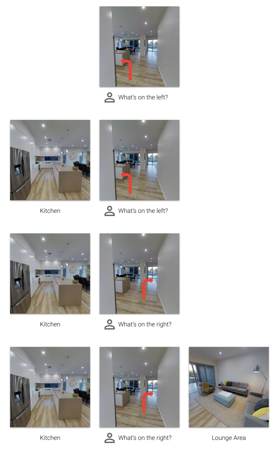
When a person navigates around an unfamiliar building, they take advantage of many visual, spatial and semantic cues to help them efficiently reach their goal. For example, even in an unfamiliar house, if they see a dining area, they can make intelligent predictions about the likely location of the kitchen and lounge areas, and therefore the expected location of common household objects. For robotic agents, taking advantage of semantic cues and statistical regularities in novel buildings is challenging. A typical approach is to implicitly learn what these cues are, and how to use them for navigation tasks, in an end-to-end manner via model-free reinforcement learning. However, navigation cues learned in this way are expensive to learn, hard to inspect, and difficult to re-use in another agent without learning again from scratch.

People navigating in unfamiliar buildings can take advantage of visual, spatial and semantic cues to predict what’s around a corner. A computational model with this capability is a visual world model.

An appealing alternative for robotic navigation and planning agents is to use a world model to encapsulate rich and meaningful information about their surroundings, which enables an agent to make specific predictions about actionable outcomes within their environment. Such models have seen widespread interest in robotics, simulation, and reinforcement learning with impressive results, including finding the first known solution for a simulated 2D car racing task, and achieving human-level performance in Atari games. However, game environments are still relatively simple compared to the complexity and diversity of real-world environments.

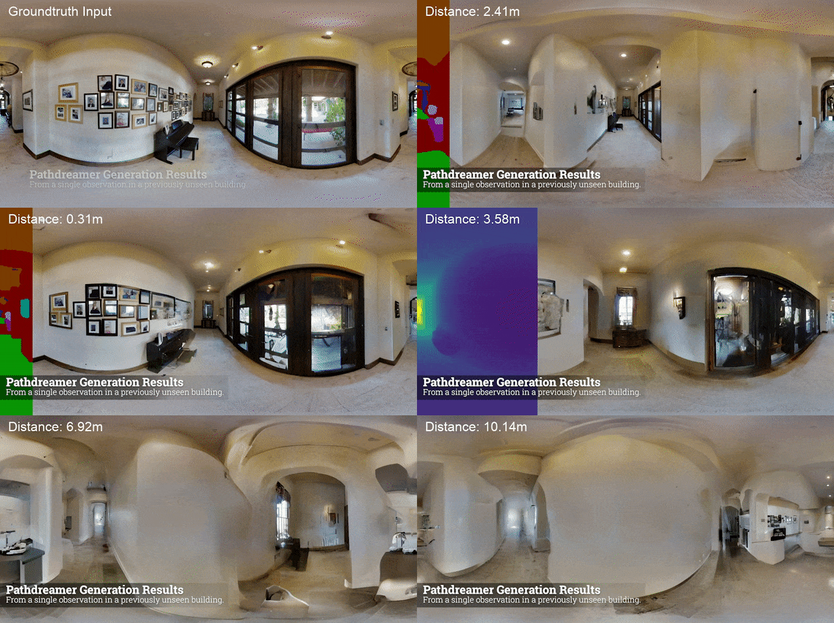
In “Pathdreamer: A World Model for Indoor Navigation”, published at ICCV 2021, we present a world model that generates high-resolution 360º visual observations of areas of a building unseen by an agent, using only limited seed observations and a proposed navigation trajectory. As illustrated in the video below, the Pathdreamer model can synthesize an immersive scene from a single viewpoint, predicting what an agent might see if it moved to a new viewpoint or even a completely unseen area, such as around a corner. Beyond potential applications in video editing and bringing photos to life, solving this task promises to codify knowledge about human environments to benefit robotic agents navigating in the real world. For example, a robot tasked with finding a particular room or object in an unfamiliar building could perform simulations using the world model to identify likely locations before physically searching anywhere. World models such as Pathdreamer can also be used to increase the amount of training data for agents, by training agents in the model.

Provided with just a single observation (RGB, depth, and segmentation) and a proposed navigation trajectory as input, Pathdreamer synthesizes high resolution 360º observations up to 6-7 meters away from the original location, including around corners. For more results, please refer to the full video.

How Does Pathdreamer Work?
Pathdreamer takes as input a sequence of one or more previous observations, and generates predictions for a trajectory of future locations, which may be provided up front or iteratively by the agent interacting with the returned observations. Both inputs and predictions consist of RGB, semantic segmentation, and depth images. Internally, Pathdreamer uses a 3D point cloud to represent surfaces in the environment. Points in the cloud are labelled with both their RGB color value and their semantic segmentation class, such as wall, chair or table.

To predict visual observations in a new location, the point cloud is first re-projected into 2D at the new location to provide ‘guidance’ images, from which Pathdreamer generates realistic high-resolution RGB, semantic segmentation and depth. As the model ‘moves’, new observations (either real or predicted) are accumulated in the point cloud. One advantage of using a point cloud for memory is temporal consistency — revisited regions are rendered in a consistent manner to previous observations.

Internally, Pathdreamer represents surfaces in the environment via a 3D point cloud containing both semantic labels (top) and RGB color values (bottom). To generate a new observation, Pathdreamer ‘moves’ through the point cloud to the new location and uses the re-projected point cloud image for guidance.

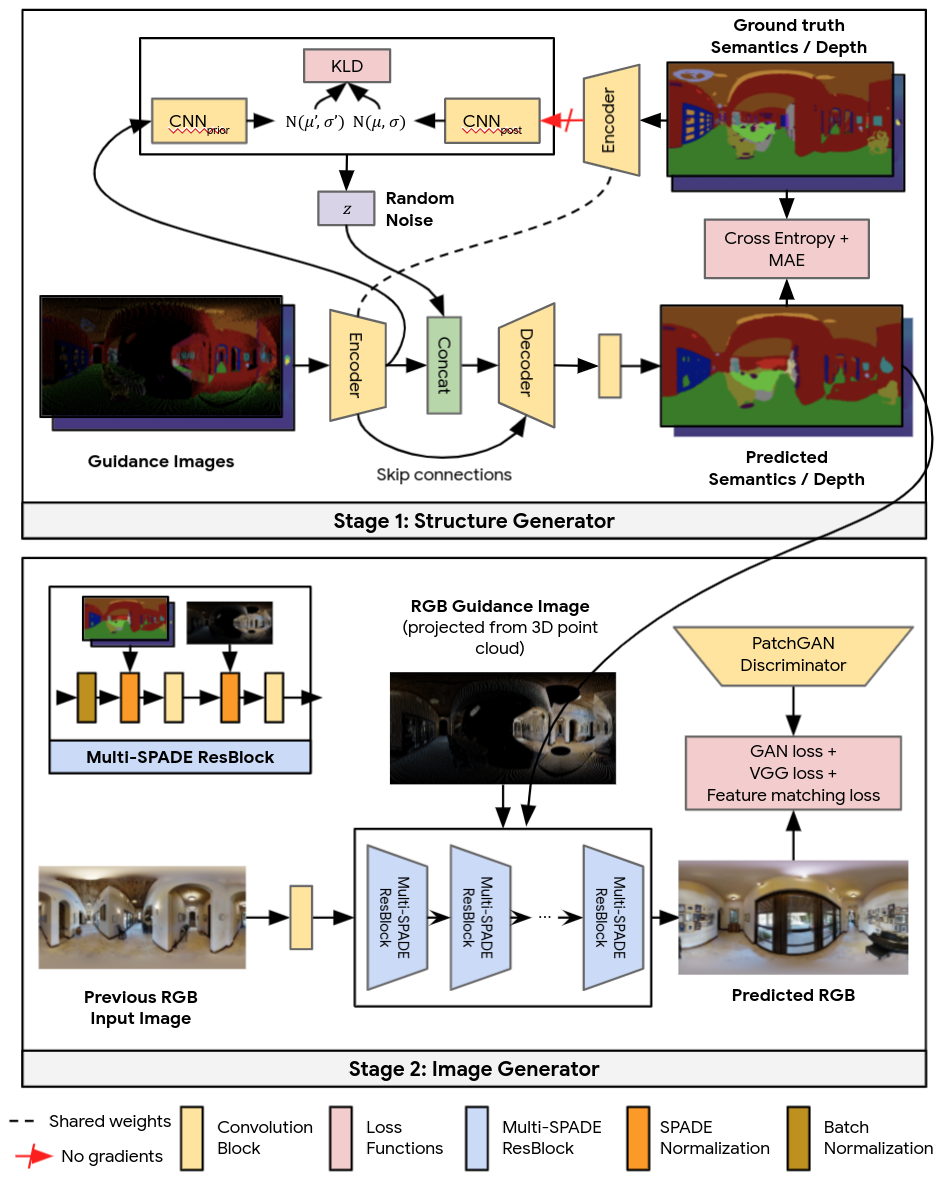
To convert guidance images into plausible, realistic outputs Pathdreamer operates in two stages: the first stage, the structure generator, creates segmentation and depth images, and the second stage, the image generator, renders these into RGB outputs. Conceptually, the first stage provides a plausible high-level semantic representation of the scene, and the second stage renders this into a realistic color image. Both stages are based on convolutional neural networks.

Pathdreamer operates in two stages: the first stage, the structure generator, creates segmentation and depth images, and the second stage, the image generator, renders these into RGB outputs. The structure generator is conditioned on a noise variable to enable the model to synthesize diverse scenes in areas of high uncertainty.

Diverse Generation Results
In regions of high uncertainty, such as an area predicted to be around a corner or in an unseen room, many different scenes are possible. Incorporating ideas from stochastic video generation, the structure generator in Pathdreamer is conditioned on a noise variable, which represents the stochastic information about the next location that is not captured in the guidance images. By sampling multiple noise variables, Pathdreamer can synthesize diverse scenes, allowing an agent to sample multiple plausible outcomes for a given trajectory. These diverse outputs are reflected not only in the first stage outputs (semantic segmentation and depth images), but in the generated RGB images as well.

Pathdreamer is capable of generating multiple diverse and plausible images for regions of high uncertainty. Guidance images on the leftmost column represent pixels that were previously seen by the agent. Black pixels represent regions that were previously unseen, for which Pathdreamer renders diverse outputs by sampling multiple random noise vectors. In practice, the generated output can be informed by new observations as the agent navigates the environment.

Pathdreamer is trained with images and 3D environment reconstructions from Matterport3D, and is capable of synthesizing realistic images as well as continuous video sequences. Because the output imagery is high-resolution and 360º, it can be readily converted for use by existing navigation agents for any camera field of view. For more details and to try out Pathdreamer yourself, we recommend taking a look at our open source code.

Application to Visual Navigation Tasks
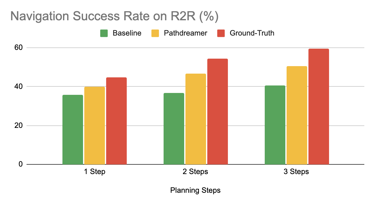
As a visual world model, Pathdreamer shows strong potential to improve performance on downstream tasks. To demonstrate this, we apply Pathdreamer to the task of Vision-and-Language Navigation (VLN), in which an embodied agent must follow a natural language instruction to navigate to a location in a realistic 3D environment. Using the Room-to-Room (R2R) dataset, we conduct an experiment in which an instruction-following agent plans ahead by simulating many possible navigable trajectory through the environment, ranking each against the navigation instructions, and choosing the best ranked trajectory to execute. Three settings are considered. In the Ground-Truth setting, the agent plans by interacting with the actual environment, i.e. by moving. In the Baseline setting, the agent plans ahead without moving by interacting with a navigation graph that encodes the navigable routes within the building, but does not provide any visual observations. In the Pathdreamer setting, the agent plans ahead without moving by interacting with the navigation graph and also receives corresponding visual observations generated by Pathdreamer.

When planning ahead for three steps (approximately 6m), in the Pathdreamer setting the VLN agent achieves a navigation success rate of 50.4%, significantly higher than the 40.6% success rate in the Baseline setting without Pathdreamer. This suggests that Pathdreamer encodes useful and accessible visual, spatial and semantic knowledge about real-world indoor environments. As an upper bound illustrating the performance of a perfect world model, under the Ground-Truth setting (planning by moving) the agent’s success rate is 59%, although we note that this setting requires the agent to expend significant time and resources to physically explore many trajectories, which would likely be prohibitively costly in a real-world setting.

We evaluate several planning settings for an instruction-following agent using the Room-to-Room (R2R) dataset. Planning ahead using a navigation graph with corresponding visual observations synthesized by Pathdreamer (Pathdreamer setting) is more effective than planning ahead using the navigation graph alone (Baseline setting), capturing around half the benefit of planning ahead using a world model that perfectly matches reality (Ground-Truth setting).

Conclusions and Future Work
These results showcase the promise of using world models such as Pathdreamer for complicated embodied navigation tasks. We hope that Pathdreamer will help unlock model-based approaches to challenging embodied navigation tasks such as navigating to specified objects and VLN.

Applying Pathdreamer to other embodied navigation tasks such as Object-Nav, continuous VLN, and street-level navigation are natural directions for future work. We also envision further research on improved architecture and modeling directions for the Pathdreamer model, as well as testing it on more diverse datasets, including but not limited to outdoor environments. To explore Pathdreamer in more detail, please visit our GitHub repository.

Acknowledgements
This project is a collaboration with Jason Baldridge, Honglak Lee, and Yinfei Yang. We thank Austin Waters, Noah Snavely, Suhani Vora, Harsh Agrawal, David Ha, and others who provided feedback throughout the project. We are also grateful for general support from Google Research teams. Finally, we thank Tom Small for creating the animation in the third figure.

Source: Google AI Blog


Announcing WIT: A Wikipedia-Based Image-Text Dataset

Multimodal visio-linguistic models rely on rich datasets in order to model the relationship between images and text. Traditionally, these datasets have been created by either manually captioning images, or crawling the web and extracting the alt-text as the caption. While the former approach tends to result in higher quality data, the intensive manual annotation process limits the amount of data that can be created. On the other hand, the automated extraction approach can lead to bigger datasets, but these require either heuristics and careful filtering to ensure data quality or scaling-up models to achieve strong performance. An additional shortcoming of existing datasets is the dearth of coverage in non-English languages. This naturally led us to ask: Can one overcome these limitations and create a high-quality, large-sized, multilingual dataset with a variety of content?

Today we introduce the Wikipedia-Based Image Text (WIT) Dataset, a large multimodal dataset, created by extracting multiple different text selections associated with an image from Wikipedia articles and Wikimedia image links. This was accompanied by rigorous filtering to only retain high quality image-text sets. As detailed in “WIT: Wikipedia-based Image Text Dataset for Multimodal Multilingual Machine Learning”, presented at SIGIR ‘21, this resulted in a curated set of 37.5 million entity-rich image-text examples with 11.5 million unique images across 108 languages. The WIT dataset is available for download and use under the Creative Commons license. We are also excited to announce that we are hosting a competition with the WIT dataset in Kaggle in collaboration with Wikimedia Research and other external collaborators.

Dataset   Images     Text     Contextual Text     Languages  
Flickr30K 32K 158K - < 8
SBU Captions     1M 1M - 1
MS-COCO 330K 1.5M - < 4; 7 (test only)
CC-3M
CC-12M
3.3M
12M
3.3M
12M
-
-
1
1
WIT 11.5M 37.5M ~119M 108
WIT’s increased language coverage and larger size relative to previous datasets.

The unique advantages of the WIT dataset are:

  1. Size: WIT is the largest multimodal dataset of image-text examples that is publicly available.
  2. Multilingual: With 108 languages, WIT has 10x or more languages than any other dataset.
  3. Contextual information: Unlike typical multimodal datasets, which have only one caption per image, WIT includes many page-level and section-level contextual information.
  4. Real world entities: Wikipedia, being a broad knowledge-base, is rich with real world entities that are represented in WIT.
  5. Challenging test set: In our recent work accepted at EMNLP, all state-of-the-art models demonstrated significantly lower performance on WIT vs. traditional evaluation sets (e.g., ~30 point drop in recall).

Generating the Dataset
The main goal of WIT was to create a large dataset without sacrificing on quality or coverage of concepts. Thus, we started by leveraging the largest online encyclopedia available today: Wikipedia.

For an example of the depth of information available, consider the Wikipedia page for Half Dome (Yosemite National Park, CA). As shown below, the article has numerous interesting text captions and relevant contextual information for the image, such as the page title, main page description, and other contextual information and metadata.

Example wikipedia page with various image-associated text selections and contexts we can extract. From the Wikipedia page for Half Dome : Photo by DAVID ILIFF. License: CC BY-SA 3.0.
Example of the Wikipedia page for this specific image of Half Dome. From the Wikipedia page for Half Dome : Photo by DAVID ILIFF. License: CC BY-SA 3.0.

We started by selecting Wikipedia pages that have images, then extracted various image-text associations and surrounding contexts. To further refine the data, we performed a rigorous filtering process to ensure data quality. This included text-based filtering to ensure caption availability, length and quality (e.g., by removing generic default filler text); image-based filtering to ensure each image is a certain size with permissible licensing; and finally, image-and-text-entity–based filtering to ensure suitability for research (e.g., excluding those classified as hate speech). We further randomly sampled image-caption sets for evaluation by human editors, who overwhelmingly agreed that 98% of the samples had good image-caption alignment.

Highly Multilingual
With data in 108 languages, WIT is the first large-scale, multilingual, multimodal dataset.

# of Image-Text Sets   Unique Languages   # of Images   Unique Languages  
> 1M 9 > 1M 6
500K - 1M 10 500K - 1M 12
  100K - 500K   36   100K - 500K   35
50K - 100K 15 50K - 100K 17
14K - 50K 38 13K - 50K 38
WIT: coverage statistics across languages.
Example of an image that is present in more than a dozen Wikipedia pages across >12 languages. From the Wikipedia page for Wolfgang Amadeus Mozart.

The First Contextual Image-Text Dataset
Most multimodal datasets only offer a single text caption (or multiple versions of a similar caption) for the given image. WIT is the first dataset to provide contextual information, which can help researchers model the effect of context on image captions as well as the choice of images.

WIT dataset example showing image-text data and additional contextual information.

In particular, key textual fields of WIT that may be useful for research include:

  • Text captions: WIT offers three different kinds of image captions. This includes the (potentially context influenced) “Reference description”, the (likely context independent) “Attribution description” and “Alt-text description”.
  • Contextual information: This includes the page title, page description, URL and local context about the Wikipedia section including the section title and text.

WIT has broad coverage across these different fields, as shown below.

Image-Text Fields of WIT     Train Val Test Total / Unique
Rows / Tuples   37.1M     261.8K     210.7K   37.6M
Unique Images 11.4M 58K 57K 11.5M
Reference Descriptions 16.9M 150K 104K   17.2M / 16.7M  
Attribution Descriptions 34.8M 193K 200K 35.2M / 10.9M
Alt-Text 5.3M 29K 29K 5.4M / 5.3M
Context Texts - - - 119.8M
Key fields of WIT include both text captions and contextual information.

A High-Quality Training Set and a Challenging Evaluation Benchmark
The broad coverage of diverse concepts in Wikipedia means that the WIT evaluation sets serve as a challenging benchmark, even for state-of-the-art models. We found that for image-text retrieval, the mean recall scores for traditional datasets were in the 80s, whereas for the WIT test set, it was in the 40s for well-resourced languages and in the 30s for the under-resourced languages. We hope this in turn can help researchers to build stronger, more robust models.

WIT Dataset and Competition with Wikimedia and Kaggle
Additionally, we are happy to announce that we are partnering with Wikimedia Research and a few external collaborators to organize a competition with the WIT test set. We are hosting this competition in Kaggle. The competition is an image-text retrieval task. Given a set of images and text captions, the task is to retrieve the appropriate caption(s) for each image.

To enable research in this area, Wikipedia has kindly made available images at 300-pixel resolution and a Resnet-50–based image embeddings for most of the training and the test dataset. Kaggle will be hosting all this image data in addition to the WIT dataset itself and will provide colab notebooks. Further, the competitors will have access to a discussion forum in Kaggle in order to share code and collaborate. This enables anyone interested in multimodality to get started and run experiments easily. We are excited and looking forward to what will result from the WIT dataset and the Wikipedia images in the Kaggle platform.

Conclusion
We believe that the WIT dataset will aid researchers in building better multimodal multilingual models and in identifying better learning and representation techniques, ultimately leading to improved Machine Learning models in real-world tasks over visio-linguistic data. For any questions, please contact [email protected]. We would love to hear about how you are using the WIT dataset.

Acknowledgements
We would like to thank our co-authors in Google Research: Jiecao Chen, Michael Bendersky and Marc Najork. We thank Beer Changpinyo, Corinna Cortes, Joshua Gang, Chao Jia, Ashwin Kakarla, Mike Lee, Zhen Li, Piyush Sharma, Radu Soricut, Ashish Vaswani, Yinfei Yang, and our reviewers for their insightful feedback and comments.

We thank Miriam Redi and Leila Zia from Wikimedia Research for collaborating with us on the competition and providing image pixels and image embedding data. We thank Addison Howard and Walter Reade for helping us host this competition in Kaggle. We also thank Diane Larlus (Naver Labs Europe (NLE)), Yannis Kalantidis (NLE), Stéphane Clinchant (NLE), Tiziano Piccardi Ph.D. student at EPFL, Lucie-Aimée Kaffee PhD student at University of Southampton and Yacine Jernite (Hugging Face) for their valuable contribution towards the competition.

Source: Google AI Blog


Toward Fast and Accurate Neural Networks for Image Recognition

As neural network models and training data size grow, training efficiency is becoming an important focus for deep learning. For example, GPT-3 demonstrates remarkable capability in few-shot learning, but it requires weeks of training with thousands of GPUs, making it difficult to retrain or improve. What if, instead, one could design neural networks that were smaller and faster, yet still more accurate?

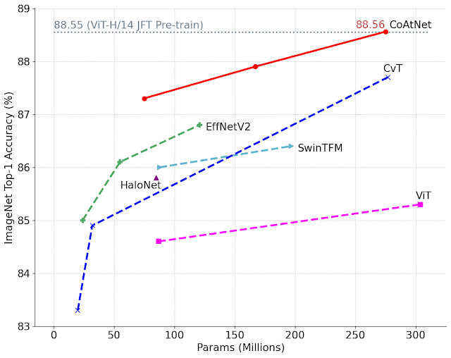
In this post, we introduce two families of models for image recognition that leverage neural architecture search, and a principled design methodology based on model capacity and generalization. The first is EfficientNetV2 (accepted at ICML 2021), which consists of convolutional neural networks that aim for fast training speed for relatively small-scale datasets, such as ImageNet1k (with 1.28 million images). The second family is CoAtNet, which are hybrid models that combine convolution and self-attention, with the goal of achieving higher accuracy on large-scale datasets, such as ImageNet21 (with 13 million images) and JFT (with billions of images). Compared to previous results, our models are 4-10x faster while achieving new state-of-the-art 90.88% top-1 accuracy on the well-established ImageNet dataset. We are also releasing the source code and pretrained models on the Google AutoML github.

EfficientNetV2: Smaller Models and Faster Training
EfficientNetV2 is based upon the previous EfficientNet architecture. To improve upon the original, we systematically studied the training speed bottlenecks on modern TPUs/GPUs and found: (1) training with very large image sizes results in higher memory usage and thus is often slower on TPUs/GPUs; (2) the widely used depthwise convolutions are inefficient on TPUs/GPUs, because they exhibit low hardware utilization; and (3) the commonly used uniform compound scaling approach, which scales up every stage of convolutional networks equally, is sub-optimal. To address these issues, we propose both a training-aware neural architecture search (NAS), in which the training speed is included in the optimization goal, and a scaling method that scales different stages in a non-uniform manner.

The training-aware NAS is based on the previous platform-aware NAS, but unlike the original approach, which mostly focuses on inference speed, here we jointly optimize model accuracy, model size, and training speed. We also extend the original search space to include more accelerator-friendly operations, such as FusedMBConv, and simplify the search space by removing unnecessary operations, such as average pooling and max pooling, which are never selected by NAS. The resulting EfficientNetV2 networks achieve improved accuracy over all previous models, while being much faster and up to 6.8x smaller.

To further speed up the training process, we also propose an enhanced method of progressive learning, which gradually changes image size and regularization magnitude during training. Progressive training has been used in image classification, GANs, and language models. This approach focuses on image classification, but unlike previous approaches that often trade accuracy for improved training speed, can slightly improve the accuracy while also significantly reducing training time. The key idea in our improved approach is to adaptively change regularization strength, such as dropout ratio or data augmentation magnitude, according to the image size. For the same network, small image size leads to lower network capacity and thus requires weak regularization; vice versa, a large image size requires stronger regularization to combat overfitting.

Progressive learning for EfficientNetV2. Here we mainly focus on three types of regularizations: data augmentation, mixup, and dropout.

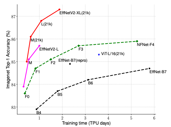
We evaluate the EfficientNetV2 models on ImageNet and a few transfer learning datasets, such as CIFAR-10/100, Flowers, and Cars. On ImageNet, EfficientNetV2 significantly outperforms previous models with about 5–11x faster training speed and up to 6.8x smaller model size, without any drop in accuracy.

EfficientNetV2 achieves much better training efficiency than prior models for ImageNet classification.

CoAtNet: Fast and Accurate Models for Large-Scale Image Recognition
While EfficientNetV2 is still a typical convolutional neural network, recent studies on Vision Transformer (ViT) have shown that attention-based transformer models could perform better than convolutional neural networks on large-scale datasets like JFT-300M. Inspired by this observation, we further expand our study beyond convolutional neural networks with the aim of finding faster and more accurate vision models.

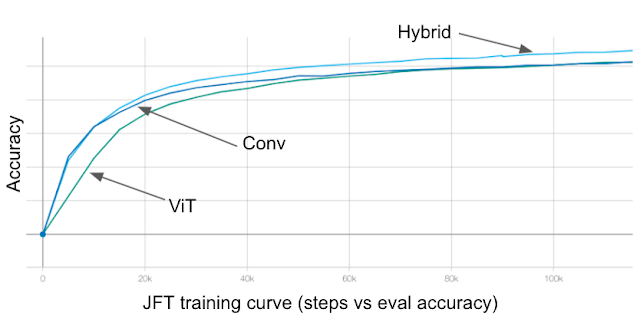
In “CoAtNet: Marrying Convolution and Attention for All Data Sizes”, we systematically study how to combine convolution and self-attention to develop fast and accurate neural networks for large-scale image recognition. Our work is based on an observation that convolution often has better generalization (i.e., the performance gap between training and evaluation) due to its inductive bias, while self-attention tends to have greater capacity (i.e., the ability to fit large-scale training data) thanks to its global receptive field. By combining convolution and self-attention, our hybrid models can achieve both better generalization and greater capacity.

Comparison between convolution, self-attention, and hybrid models. Convolutional models converge faster, ViTs have better capacity, while the hybrid models achieve both faster convergence and better accuracy.

We observe two key insights from our study: (1) depthwise convolution and self-attention can be naturally unified via simple relative attention, and (2) vertically stacking convolution layers and attention layers in a way that considers their capacity and computation required in each stage (resolution) is surprisingly effective in improving generalization, capacity and efficiency. Based on these insights, we have developed a family of hybrid models with both convolution and attention, named CoAtNets (pronounced “coat” nets). The following figure shows the overall CoAtNet network architecture:

Overall CoAtNet architecture. Given an input image with size HxW, we first apply convolutions in the first stem stage (S0) and reduce the size to H/2 x W/2. The size continues to reduce with each stage. Ln refers to the number of layers. Then, the early two stages (S1 and S2) mainly adopt MBConv building blocks consisting of depthwise convolution. The later two stages (S3 and S4) mainly adopt Transformer blocks with relative self-attention. Unlike the previous Transformer blocks in ViT, here we use pooling between stages, similar to Funnel Transformer. Finally, we apply a classification head to generate class prediction.

CoAtNet models consistently outperform ViT models and its variants across a number of datasets, such as ImageNet1K, ImageNet21K, and JFT. When compared to convolutional networks, CoAtNet exhibits comparable performance on a small-scale dataset (ImageNet1K) and achieves substantial gains as the data size increases (e.g. on ImageNet21K and JFT).

Comparison between CoAtNet and previous models after pre-training on the medium sized ImageNet21K dataset. Under the same model size, CoAtNet consistently outperforms both ViT and convolutional models. Noticeably, with only ImageNet21K, CoAtNet is able to match the performance of ViT-H pre-trained on JFT.

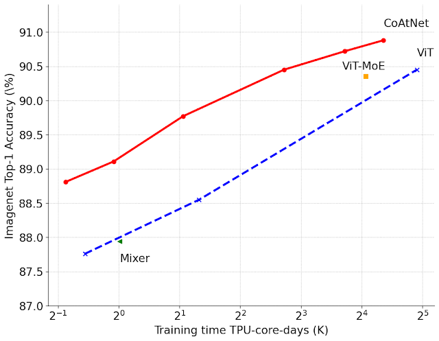
We also evaluated CoAtNets on the large-scale JFT dataset. To reach a similar accuracy target, CoAtNet trains about 4x faster than previous ViT models and more importantly, achieves a new state-of-the-art top-1 accuracy on ImageNet of 90.88%.

Comparison between CoAtNets and previous ViTs. ImageNet top-1 accuracy after pre-training on JFT dataset under different training budget. The four best models are trained on JFT-3B with about 3 billion images.

Conclusion and Future Work
In this post, we introduce two families of neural networks, named EfficientNetV2 and CoAtNet, which achieve state-of-the-art performance on image recognition. All EfficientNetV2 models are open sourced and the pretrained models are also available on the TFhub. CoAtNet models will also be open-sourced soon. We hope these new neural networks can benefit the research community and the industry. In the future we plan to further optimize these models and apply them to new tasks, such as zero-shot learning and self-supervised learning, which often require fast models with high capacity.

Acknowledgements
Special thanks to our co-authors Hanxiao Liu and Quoc Le. We also thank the Google Research, Brain Team and the open source contributors.

Source: Google AI Blog


Revisiting Mask-Head Architectures for Novel Class Instance Segmentation

Instance segmentation is the task of grouping pixels in an image into instances of individual things, and identifying those things with a class label (countable objects such as people, animals, cars, etc., and assigning unique identifiers to each, e.g., car_1 and car_2). As a core computer vision task, it is critical to many downstream applications, such as self-driving cars, robotics, medical imaging, and photo editing. In recent years, deep learning has made significant strides in solving the instance segmentation problem with architectures like Mask R-CNN. However, these methods rely on collecting a large labeled instance segmentation dataset. But unlike bounding box labels, which can be collected in 7 seconds per instance with methods like Extreme clicking, collecting instance segmentation labels (called “masks”) can take up to 80 seconds per instance, an effort that is costly and creates a high barrier to entry for this research. And a related task, pantopic segmentation, requires even more labeled data.

The partially supervised instance segmentation setting, where only a small set of classes are labeled with instance segmentation masks and the remaining (majority of) classes are labeled only with bounding boxes, is an approach that has the potential to reduce the dependence on manually-created mask labels, thereby significantly lowering the barriers to developing an instance segmentation model. However this partially supervised approach also requires a stronger form of model generalization to handle novel classes not seen at training time—e.g., training with only animal masks and then tasking the model to produce accurate instance segmentations for buildings or plants. Further, naïve approaches, such as training a class-agnostic Mask R-CNN, while ignoring mask losses for any instances that don’t have mask labels, have not worked well. For example, on the typical “VOC/Non-VOC” benchmark, where one trains on masks for a subset of 20 classes in COCO (called “seen classes”) and is tested on the remaining 60 classes (called “unseen classes”), a typical Mask R-CNN with Resnet-50 backbone gets to only ~18% mask mAP (mean Average Precision, higher is better) on unseen classes, whereas when fully supervised it can achieve a much higher >34% mask mAP on the same set.

In “The surprising impact of mask-head architecture on novel class segmentation”, to be presented at ICCV 2021, we identify the main culprits for Mask R-CNN’s poor performance on novel classes and propose two easy-to-implement fixes (one training protocol fix, one mask-head architecture fix) that work in tandem to close the gap to fully supervised performance. We show that our approach applies generally to crop-then-segment models, i.e., a Mask R-CNN or Mask R-CNN-like architecture that computes a feature representation of the entire image and then subsequently passes per-instance crops to a second-stage mask prediction network—also called a mask-head network. Putting our findings together, we propose a Mask R-CNN–based model that improves over the current state-of-the-art by a significant 4.7% mask mAP without requiring more complex auxiliary loss functions, offline trained priors, or weight transfer functions proposed by previous work. We have also open sourced the code bases for two versions of the model, called Deep-MAC and Deep-MARC, and published a colab to interactively produce masks like the video demo below.

A demo of our model, DeepMAC, which learns to predict accurate masks, given user specified boxes, even on novel classes that were not seen at training time. Try it yourself in the colab. Image credits: Chris Briggs, Wikipedia and Europeana.

Impact of Cropping Methodology in Partially Supervised Settings
An important step of crop-then-segment models is cropping—Mask R-CNN is trained by cropping a feature map as well as the ground truth mask to a bounding box corresponding to each instance. These cropped features are passed to another neural network (called a mask-head network) that computes a final mask prediction, which is then compared against the ground truth crop in the mask loss function. There are two choices for cropping: (1) cropping directly to the ground truth bounding box of an instance, or (2) cropping to bounding boxes predicted by the model (called, proposals). At test time, cropping is always performed with proposals as ground truth boxes are not assumed to be available.

Cropping to ground truth boxes vs. cropping to proposals predicted by a model during training. Standard Mask R-CNN implementations use both types of crops, but we show that cropping exclusively to ground truth boxes yields significantly stronger performance on novel categories.
We consider a general family of Mask R-CNN–like architectures with one small, but critical difference from typical Mask R-CNN training setups: we crop using ground truth boxes (instead of proposal boxes) at training time.

Typical Mask R-CNN implementations pass both types of crops to the mask head. However, this choice has traditionally been considered an unimportant implementation detail, because it does not affect performance significantly in the fully supervised setting. In contrast, for partially supervised settings, we find that cropping methodology plays a significant role—while cropping exclusively to ground truth boxes during training doesn’t change the results significantly in the fully supervised setting, it has a surprising and dramatic positive impact in the partially supervised setting, performing significantly better on unseen classes.

Performance of Mask R-CNN on unseen classes when trained with either proposals and ground truth (the default) or with only ground truth boxes. Training mask heads with only ground truth boxes yields a significant boost to performance on unseen classes, upwards of 9% mAP. We report performance with the ResNet-101-FPN backbone.

Unlocking the Full Generalization Potential of the Mask Head
Even more surprisingly, the above approach unlocks a novel phenomenon—with cropping-to-ground truth enabled during training, the mask head of Mask R-CNN takes on a disproportionate role in the ability of the model to generalize to unseen classes. As an example, in the following figure, we compare models that all have cropping-to-ground-truth enabled, but different out-of-the-box mask-head architectures on a parking meter, cell phone, and pizza (classes unseen during training).

Mask predictions for unseen classes with four different mask-head architectures (from left to right: ResNet-4, ResNet-12, ResNet-20, Hourglass-20, where the number refers to the number of layers of the neural network). Despite never having seen masks from the ‘parking meter’, ‘pizza’ or ‘mobile phone’ class, the rightmost mask-head architecture can segment these classes correctly. From left to right, we show better mask-head architectures predicting better masks. Moreover, this difference is only apparent when evaluating on unseen classes — if we evaluate on seen classes, all four architectures exhibit similar performance.

Particularly notable is that these differences between mask-head architectures are not as obvious in the fully supervised setting. Incidentally, this may explain why previous works in instance segmentation have almost exclusively used shallow (i.e., low number of layers) mask heads, as there has been no benefit to the added complexity. Below we compare the mask mAP of three different mask-head architectures on seen versus unseen classes. All three models do equally well on the set of seen classes, but the deep hourglass mask heads stand out when applied to unseen classes. We find hourglass mask heads to be the best among the architectures we tried and we use hourglass mask heads with 50 or more layers to get the best results.

Performance of ResNet-4, Hourglass-10 and Hourglass-52 mask-head architectures on seen and unseen classes. There is a significant difference in performance on unseen classes, even though the performance on seen classes barely changes.

Finally, we show that our findings are general, holding for a variety of backbones (e.g., ResNet, SpineNet, Hourglass) and detector architectures including anchor-based and anchor-free detectors and even when there is no detector at all.

Putting It Together
To achieve the best result, we combined the above findings: We trained a Mask R-CNN model with cropping-to-ground-truth enabled and a deep Hourglass-52 mask head with a SpineNet backbone on high resolution images (1280x1280). We call this model Deep-MARC (Deep Mask heads Above R-CNN). Without using any offline training or other hand-crafted priors, Deep-MARC exceeds previous state-of-the-art models by > 4.5% (absolute) mask mAP. Demonstrating the general nature of this approach, we also see strong results with a CenterNet-based (as opposed to Mask R-CNN-based) model (called Deep-MAC), which also exceeds the previous state of the art.

Comparison of Deep-MAC and Deep-MARC to other partially supervised instance segmentation approaches like MaskX R-CNN, ShapeMask and CPMask.

Conclusion
We develop instance segmentation models that are able to generalize to classes that were not part of the training set. We highlight the role of two key ingredients that can be applied to any crop-then-segment model (such as Mask R-CNN): (1) cropping-to-ground truth boxes during training, and (2) strong mask-head architectures. While neither of these ingredients have a large impact on the classes for which masks are available during training, employing both leads to significant improvement on novel classes for which masks are not available during training. Moreover, these ingredients are sufficient for achieving state-of-the-art-performance on the partially-supervised COCO benchmark. Finally, our findings are general and may also have implications for related tasks, such as panoptic segmentation and pose estimation.

Acknowledgements
We thank our co-authors Zhichao Lu, Siyang Li, and Vivek Rathod. We thank David Ross and our anonymous ICCV reviewers for their comments which played a big part in improving this research.

Source: Google AI Blog