Author Archives: Google AI

Practical Differentially Private Clustering

Over the last several years, progress has been made on privacy-safe approaches for handling sensitive data, for example, while discovering insights into human mobility and through use of federated analytics such as RAPPOR. In 2019, we released an open source library to enable developers and organizations to use techniques that provide differential privacy, a strong and widely accepted mathematical notion of privacy. Differentially-private data analysis is a principled approach that enables organizations to learn and release insights from the bulk of their data while simultaneously providing a mathematical guarantee that those results do not allow any individual user's data to be distinguished or re-identified.

In this post, we consider the following basic problem: Given a database containing several attributes about users, how can one create meaningful user groups and understand their characteristics? Importantly, if the database at hand contains sensitive user attributes, how can one reveal these group characteristics without compromising the privacy of individual users?

Such a task falls under the broad umbrella of clustering, a fundamental building block in unsupervised machine learning. A clustering method partitions the data points into groups and provides a way to assign any new data point to a group with which it is most similar. The k-means clustering algorithm has been one such influential clustering method. However, when working with sensitive datasets, it can potentially reveal significant information about individual data points, putting the privacy of the corresponding user at risk.

Today, we announce the addition of a new differentially private clustering algorithm to our differential privacy library, which is based on privately generating new representative data points. We evaluate its performance on multiple datasets and compare to existing baselines, finding competitive or better performance.

K-means Clustering
Given a set of data points, the goal of k-means clustering is to identify (at most) k points, called cluster centers, so as to minimize the loss given by the sum of squared distances of the data points from their closest cluster center. This partitions the set of data points into k groups. Moreover, any new data point can be assigned to a group based on its closest cluster center. However, releasing the set of cluster centers has the potential to leak information about particular users — for example, consider a scenario where a particular data point is significantly far from the rest of the points, so the standard k-means clustering algorithm returns a cluster center at this single point, thereby revealing sensitive information about this single point. To address this, we design a new algorithm for clustering with the k-means objective within the framework of differential privacy.

A Differentially Private Algorithm
In “Locally Private k-Means in One Round”, published at ICML 2021, we presented a differentially private algorithm for clustering data points. That algorithm had the advantage of being private in the local model, where the user’s privacy is protected even from the central server performing the clustering. However, any such approach necessarily incurs a significantly larger loss than approaches using models of privacy that require trusting a central server.1

Here, we present a similarly inspired clustering algorithm that works in the central model of differential privacy, where the central server is trusted to have complete access to the raw data, and the goal is to compute differentially private cluster centers, which do not leak information about individual data points. The central model is the standard model for differential privacy, and algorithms in the central model can be more easily substituted in place of their non-private counterparts since they do not require changes to the data collection process. The algorithm proceeds by first generating, in a differentially private manner, a core-set that consists of weighted points that “represent” the data points well. This is followed by executing any (non-private) clustering algorithm (e.g., k-means++) on this privately generated core-set.

At a high level, the algorithm generates the private core-set by first using random-projection–based locality-sensitive hashing (LSH) in a recursive manner2 to partition the points into “buckets” of similar points, and then replacing each bucket by a single weighted point that is the average of the points in the bucket, with a weight equal to the number of points in the same bucket. As described so far, though, this algorithm is not private. We make it private by performing each operation in a private manner by adding noise to both the counts and averages of points within a bucket.

This algorithm satisfies differential privacy because each point’s contributions to the bucket counts and the bucket averages are masked by the added noise, so the behavior of the algorithm does not reveal information about any individual point. There is a tradeoff with this approach: if the number of points in the buckets is too large, then individual points will not be well-represented by points in the core-set, whereas if the number of points in a bucket is too small, then the added noise (to the counts and averages) will become significant in comparison to the actual values, leading to poor quality of the core-set. This trade-off is realized with user-provided parameters in the algorithm that control the number of points that can be in a bucket.

Visual illustration of the algorithm.

Experimental Evaluation
We evaluated the algorithm on a few benchmark datasets, comparing its performance to that of the (non-private) k-means++ algorithm, as well as a few other algorithms with available implementations, namely diffprivlib and dp-clustering-icml17. We use the following benchmark datasets: (i) a synthetic dataset consisting of 100,000 data points in 100 dimensions sampled from a mixture of 64 Gaussians; (ii) neural representations for the MNIST dataset on handwritten digits obtained by training a LeNet model; (iii) the UC Irvine dataset on Letter Recognition; and (iv) the UC Irvine dataset on Gas Turbine CO and NOx Emissions.3

We analyze the normalized k-means loss (mean squared distance from data points to the nearest center) while varying the number of target centers (k) for these benchmark datasets.4 The described algorithm achieves a lower loss than the other private algorithms in three out of the four datasets we consider.

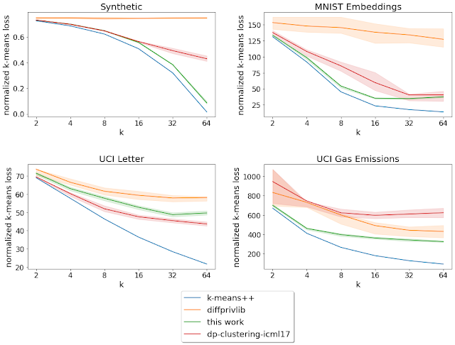
Normalized loss for varying k = number of target clusters (lower is better). The solid curves denote the mean over the 20 runs, and the shaded region denotes the 25-75th percentile range.

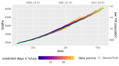
Moreover, for datasets with specified ground-truth labels (i.e., known groupings), we analyze the cluster label accuracy, which is the accuracy of the labeling obtained by assigning the most frequent ground-truth label in each cluster found by the clustering algorithm to all points in that cluster. Here, the described algorithm performs better than other private algorithms for all the datasets with pre-specified ground-truth labels that we consider.

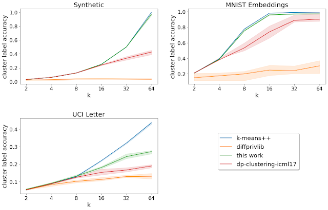
Cluster label accuracy for varying k = number of target clusters (higher is better). The solid curves denote the mean over the 20 runs, and the shaded region denotes the 25-75th percentile range.

Limitations and Future Directions
There are a couple of limitations to consider when using this or any other library for private clustering.

  1. It is important to separately account for the privacy loss in any preprocessing (e.g., centering the data points or rescaling the different coordinates) done before using the private clustering algorithm. So, we hope to provide support for differentially private versions of commonly used preprocessing methods in the future and investigate changes so that the algorithm performs better with data that isn’t necessarily preprocessed.
  2. The algorithm described requires a user-provided radius, such that all data points lie within a sphere of that radius. This is used to determine the amount of noise that is added to the bucket averages. Note that this differs from diffprivlib and dp-clustering-icml17 which take in different notions of bounds of the dataset (e.g., a minimum and maximum of each coordinate). For the sake of our experimental evaluation, we calculated the relevant bounds non-privately for each dataset. However, when running the algorithms in practice, these bounds should generally be privately computed or provided without knowledge of the dataset (e.g., using the underlying range of the data). Although, note that in case of the algorithm described, the provided radius need not be exactly correct; any data points outside of the provided radius are replaced with the closest points that are within the sphere of that radius.

Conclusion
This work proposes a new algorithm for computing representative points (cluster centers) within the framework of differential privacy. With the rise in the amount of datasets collected around the world, we hope that our open source tool will help organizations obtain and share meaningful insights about their datasets, with the mathematical assurance of differential privacy.

Acknowledgements
We thank Christoph Dibak, Badih Ghazi, Miguel Guevara, Sasha Kulankhina, Ravi Kumar, Pasin Manurangsi, Jane Shapiro, Daniel Simmons-Marengo, Yurii Sushko, and Mirac Vuslat Basaran for their help.


1As shown by Uri Stemmer in Locally private k-means clustering (SODA 2020). 
2This is similar to work on LSH Forest, used in the context of similarity-search queries. 
3Datasets (iii) and (iv) were centered to have mean zero before evaluating the algorithms. 
4Evaluation done for fixed privacy parameters ε = 1.0 and δ = 1e-6. Note that dp-clustering-icml17 works in the pure differential privacy model (namely, with δ = 0); k-means++, of course, has no privacy parameters. 

Source: Google AI Blog


Predicting Spreadsheet Formulas from Semi-structured Contexts

Hundreds of millions of people use spreadsheets, and formulas in those spreadsheets allow users to perform sophisticated analyses and transformations on their data. Although formula languages are simpler than general-purpose programming languages, writing these formulas can still be tedious and error-prone, especially for end-users. We've previously developed tools to understand patterns in spreadsheet data to automatically fill missing values in a column, but they were not built to support the process of writing formulas.

In "SpreadsheetCoder: Formula Prediction from Semi-structured Context", published at ICML 2021, we describe a new model that learns to automatically generate formulas based on the rich context around a target cell. When a user starts writing a formula with the “=” sign in a target cell, the system generates possible relevant formulas for that cell by learning patterns of formulas in historical spreadsheets. The model uses the data present in neighboring rows and columns of the target cell as well as the header row as context. It does this by first embedding the contextual structure of a spreadsheet table, consisting of neighboring and header cells, and then generates the desired spreadsheet formula using this contextual embedding. The formula is generated as two components: 1) the sequence of operators (e.g., SUM, IF, etc.), and 2) the corresponding ranges on which the operators are applied (e.g., “A2:A10”). The feature based on this model is now generally available to Google Sheets users.

Given the user’s intent to enter a formula in cells B7, C7, and D7, the system automatically infers the most likely formula the user might want to write in those cells.
Given the target cell (D4), the model uses the header and surrounding cell values as context to generate the target formula consisting of the corresponding sequence of operators and range.

Model Architecture
The model uses an encoder-decoder architecture that allows the flexibility to embed multiple types of contextual information (such as that contained in neighboring rows, columns, headers, etc.) in the encoder, which the decoder can use to generate desired formulas. To compute the embedding of the tabular context, it first uses a BERT-based architecture to encode several rows above and below the target cell (together with the header row). The content in each cell includes its data type (such as numeric, string, etc.) and its value, and the cell contents present in the same row are concatenated together into a token sequence to be embedded using the BERT encoder. Similarly, it encodes several columns to the left and to the right of the target cell. Finally, it performs a row-wise and column-wise convolution on the two BERT encoders to compute an aggregated representation of the context.

The decoder uses a long short-term memory (LSTM) architecture to generate the desired target formula as a sequence of tokens by first predicting a formula-sketch (consisting of formula operators without ranges) and then generating the corresponding ranges using cell addresses relative to the target cell. It additionally leverages an attention mechanism to compute attention vectors over the header and cell data, which are concatenated to the LSTM output layer before making the predictions.

The overall architecture of the formula prediction model.

In addition to the data present in neighboring rows and columns, the model also leverages additional information from the high-level sheet structure, such as headers. Using TPUs for model predictions, we ensure low latency on generating formula suggestions and are able to handle more requests on fewer machines.

Leveraging the high-level spreadsheet structure, the model can learn ranges that span thousands of rows.

Results
In the paper, we trained the model on a corpus of spreadsheets created by and shared with Googlers. We split 46k Google Sheets with formulas into 42k for training, 2.3k for validation, and 1.7k for testing. The model achieves a 42.5% top-1 full-formula accuracy, and 57.4% top-1 formula-sketch accuracy, both of which we find high enough to be practically useful in our initial user studies. We perform an ablation study, in which we test several simplifications of the model by removing different components, and find that having row- and column-based context embedding as well as header information is important for models to perform well.

The performance of different ablations of our model with increasing lengths of the target formula.

Conclusion
Our model illustrates the benefits of learning to represent the two-dimensional relational structure of the spreadsheet tables together with high-level structural information, such as table headers, to facilitate formula predictions. There are several exciting research directions, both in terms of designing new model architectures to incorporate more tabular structure as well as extending the model to support more applications such as bug detection and automated chart creation in spreadsheets. We are also looking forward to seeing how users use this feature and learning from feedback for future improvements.

Acknowledgements
We gratefully acknowledge the key contributions of the other team members, including Alexander Burmistrov, Xinyun Chen, Hanjun Dai, Prashant Khurana, Petros Maniatis, Rahul Srinivasan, Charles Sutton, Amanuel Taddesse, Peilun Zhang, and Denny Zhou.

Source: Google AI Blog


How Underspecification Presents Challenges for Machine Learning

Machine learning (ML) models are being used more widely today than ever before and are becoming increasingly impactful. However, they often exhibit unexpected behavior when they are used in real-world domains. For example, computer vision models can exhibit surprising sensitivity to irrelevant features, while natural language processing models can depend unpredictably on demographic correlations not directly indicated by the text. Some reasons for these failures are well-known: for example, training ML models on poorly curated data, or training models to solve prediction problems that are structurally mismatched with the application domain. Yet, even when these known problems are handled, model behavior can still be inconsistent in deployment, varying even between training runs.

In “Underspecification Presents Challenges for Credibility in Modern Machine Learning”, to be published in the Journal of Machine Learning Research, we show that a key failure mode especially prevalent in modern ML systems is underspecification. The idea behind underspecification is that while ML models are validated on held-out data, this validation is often insufficient to guarantee that the models will have well-defined behavior when they are used in a new setting. We show that underspecification appears in a wide variety of practical ML systems and suggest some strategies for mitigation.

Underspecification
ML systems have been successful largely because they incorporate validation of the model on held-out data to ensure high performance. However, for a fixed dataset and model architecture, there are often many distinct ways that a trained model can achieve high validation performance. But under standard practice, models that encode distinct solutions are often treated as equivalent because their held-out predictive performance is approximately equivalent.

Importantly, the distinctions between these models do become clear when they are measured on criteria beyond standard predictive performance, such as fairness or robustness to irrelevant input perturbations. For example, among models that perform equally well on standard validations, some may exhibit greater performance disparities between social groups than others, or rely more heavily on irrelevant information. These differences, in turn, can translate to real differences in behavior when the model is used in real-world scenarios.

Underspecification refers to this gap between the requirements that practitioners often have in mind when they build an ML model, and the requirements that are actually enforced by the ML pipeline (i.e., the design and implementation of a model). An important consequence of underspecification is that even if the pipeline could in principle return a model that meets all of these requirements, there is no guarantee that in practice the model will satisfy any requirement beyond accurate prediction on held-out data. In fact, the model that is returned may have properties that instead depend on arbitrary or opaque choices made in the implementation of the ML pipeline, such as those arising from random initialization seeds, data ordering, hardware, etc. Thus, ML pipelines that do not include explicit defects may still return models that behave unexpectedly in real-world settings.

Identifying Underspecification in Real Applications
In this work, we investigated concrete implications of underspecification in the kinds of ML models that are used in real-world applications. Our empirical strategy was to construct sets of models using nearly identical ML pipelines, to which we only applied small changes that had no practical effect on standard validation performance. Here, we focused on the random seed used to initialize training and determine data ordering. If important properties of the model can be substantially influenced by these changes, it indicates that the pipeline does not fully specify this real-world behavior. In every domain where we conducted this experiment, we found that these small changes induced substantial variation on axes that matter in real-world use.

Underspecification in Computer Vision
As an example, consider underspecification and its relationship to robustness in computer vision. A central challenge in computer vision is that deep models often suffer from brittleness under distribution shifts that humans do not find challenging. For instance, image classification models that perform well on the ImageNet benchmark are known to perform poorly on benchmarks like ImageNet-C, which apply common image corruptions, such as pixelization or motion blur, to the standard ImageNet test set.

In our experiment, we showed that model sensitivity to these corruptions is underspecified by standard pipelines. Following the strategy discussed above, we generated fifty ResNet-50 image classification models using the same pipeline and the same data. The only difference between these models was the random seed used in training. When evaluated on the standard ImageNet validation set, these models achieved practically equivalent performance. However, when the models were evaluated on different test sets in the ImageNet-C benchmark (i.e., on corrupted data), performance on some tests varied by orders of magnitude more than on standard validations. This pattern persisted for larger-scale models that were pre-trained on much larger datasets (e.g., a BiT-L model pre-trained on the 300 million image JFT-300M dataset). For these models, varying the random seed at the fine-tuning stage of training produced a similar pattern of variations.

Left: Parallel axis plots showing the variation in accuracy between identical, randomly initialized ResNet-50 models on strongly corrupted ImageNet-C data. Lines represent the performance of each model in the ensemble on classification tasks using uncorrupted test data, as well as corrupted data (pixelation, contrast, motion blur, and brightness). Given values are the deviation in accuracy from the ensemble mean, scaled by the standard deviation of accuracies on the “clean” ImageNet test set. The solid black line highlights the performance of an arbitrarily selected model to show how performance on one test may not be a good indication of performance on others. Right: Example images from the standard ImageNet test set, with corrupted versions from the ImageNet-C benchmark.

We also showed that underspecification can have practical implications in special-purpose computer vision models built for medical imaging, where deep learning models have shown great promise. We considered two research pipelines intended as precursors for medical applications: one ophthalmology pipeline for building models that detect diabetic retinopathy and referable diabetic macular edema from retinal fundus images, and one dermatology pipeline for building models to recognize common dermatological conditions from photographs of skin. In our experiments, we considered pipelines that were validated only on randomly held-out data.

We then stress-tested models produced by these pipelines on practically important dimensions. For the ophthalmology pipeline, we tested how models trained with different random seeds performed when applied to images taken from a new camera type not encountered during training. For the dermatology pipeline, the stress test was similar, but for patients with different estimated skin types (i.e., non-dermatologist evaluation of tone and response to sunlight). In both cases, we found that standard validations were not enough to fully specify the trained model’s performance on these axes. In the ophthalmology application, the random seed used in training induced wider variability in performance on a new camera type than would have been expected from standard validations, and in the dermatology application, the random seed induced similar variation in performance in skin-type subgroups, even though the overall performance of the models was stable across seeds.

These results reiterate that standard hold-out testing alone is not sufficient to ensure acceptable model behavior in medical applications, underscoring the need for expanded testing protocols for ML systems intended for application in the medical domain. In the medical literature, such validations are termed "external validation" and have historically been part of reporting guidelines such as STARD and TRIPOD. These are being emphasized in updates such as STARD-AI and TRIPOD-AI. Finally, as part of regulated medical device development processes (see, e.g., US and EU regulations), there are other forms of safety and performance related considerations, such as mandatory compliance to standards for risk management, human factors engineering, clinical validations and accredited body reviews, that aim to ensure acceptable medical application performance.

Relative variability of medical imaging models on stress tests, using the same conventions as the figure above. Top left: Variation in AUC between diabetic retinopathy classification models trained using different random seeds when evaluated on images from different camera types. In this experiment, camera type 5 was not encountered during training. Bottom left: Variation in accuracy between skin condition classification models trained using different random seeds when evaluated on different estimated skin types (approximated by dermatologist-trained laypersons from retrospective photographs and potentially subject to labeling errors). Right: example images from the original test set (left) and the stress test set (right).

Underspecification in Other Applications

The cases discussed above are a small subset of models that we probed for underspecification. Other cases we examined include:

  • Natural Language Processing: We showed that on a variety of NLP tasks, underspecification affected how models derived from BERT-processed sentences. For example, depending on the random seed, a pipeline could produce a model that depends more or less on correlations involving gender (e.g., between gender and occupation) when making predictions.
  • Acute Kidney Injury (AKI) prediction: We showed that underspecification affects reliance on operational versus physiological signals in AKI prediction models based on electronic health records.
  • Polygenic Risk Scores (PRS): We showed that underspecification influences the ability for (PRS) models, which predict clinical outcomes based on patient genomic data, to generalize across different patient populations.

In each case, we showed that these important properties are left ill-defined by standard training pipelines, making them sensitive to seemingly innocuous choices.

Conclusion
Addressing underspecification is a challenging problem. It requires full specification and testing of requirements for a model beyond standard predictive performance. Doing this well needs full engagement with the context in which the model will be used, an understanding of how the training data were collected, and often, incorporation of domain expertise when the available data fall short. These aspects of ML system design are often underemphasized in ML research today. A key goal of this work is to show how underinvestment in this area can manifest concretely, and to encourage the development of processes for fuller specification and testing of ML pipelines.

Some important first steps in this area are to specify stress testing protocols for any applied ML pipeline that is meant to see real-world use. Once these criteria are codified in measurable metrics, a number of different algorithmic strategies may be useful for improving them, including data augmentation, pretraining, and incorporation of causal structure. It should be noted, however, that ideal stress testing and improvement processes will usually require iteration: both the requirements for ML systems, and the world in which they are used, are constantly changing.

Acknowledgements
We would like to thank all of our co-authors, Dr. Nenad Tomasev (DeepMind), Prof. Finale Doshi-Velez (Harvard SEAS), UK Biobank, and our partners, EyePACS, Aravind Eye Hospital and Sankara Nethralaya.

Source: Google AI Blog


SimVLM: Simple Visual Language Model Pre-training with Weak Supervision

Vision-language modeling grounds language understanding in corresponding visual inputs, which can be useful for the development of important products and tools. For example, an image captioning model generates natural language descriptions based on its understanding of a given image. While there are various challenges to such cross-modal work, significant progress has been made in the past few years on vision-language modeling thanks to the adoption of effective vision-language pre-training (VLP). This approach aims to learn a single feature space from both visual and language inputs, rather than learning two separate feature spaces, one each for visual inputs and another for language inputs. For this purpose, existing VLP often leverages an object detector, like Faster R-CNN, trained on labeled object detection datasets to isolate regions-of-interest (ROI), and relies on task-specific approaches (i.e., task-specific loss functions) to learn representations of images and texts jointly. Such approaches require annotated datasets or time to design task-specific approaches, and so, are less scalable.

To address this challenge, in “SimVLM: Simple Visual Language Model Pre-training with Weak Supervision”, we propose a minimalist and effective VLP, named SimVLM, which stands for “Simple Visual Language Model”. SimVLM is trained end-to-end with a unified objective, similar to language modeling, on a vast amount of weakly aligned image-text pairs (i.e., the text paired with an image is not necessarily a precise description of the image). The simplicity of SimVLM enables efficient training on such a scaled dataset, which helps the model to achieve state-of-the-art performance across six vision-language benchmarks. Moreover, SimVLM learns a unified multimodal representation that enables strong zero-shot cross-modality transfer without fine-tuning or with fine-tuning only on text data, including for tasks such as open-ended visual question answering, image captioning and multimodal translation.

Model and Pre-training Procedure
Unlike existing VLP methods that adopt pre-training procedures similar to masked language modeling (like in BERT), SimVLM adopts the sequence-to-sequence framework and is trained with a one prefix language model (PrefixLM) objective, which receives the leading part of a sequence (the prefix) as inputs, then predicts its continuation. For example, given the sequence “A dog is chasing after a yellow ball”, the sequence is randomly truncated to “A dog is chasing” as the prefix, and the model will predict its continuation. The concept of a prefix similarly applies to images, where an image is divided into a number of “patches”, then a subset of those patches are sequentially fed to the model as inputs—this is called an “image patch sequence”. In SimVLM, for multimodal inputs (e.g., images and their captions), the prefix is a concatenation of both the image patch sequence and prefix text sequence, received by the encoder. The decoder then predicts the continuation of the textual sequence. Compared to prior VLP models combining several pre-training losses, the PrefixLM loss is the only training objective and significantly simplifies the training process. This approach for SimVLM maximizes its flexibility and universality in accommodating different task setups.

Finally, due to its success for both language and vision tasks, like BERT and ViT, we adopt the Transformer architecture as the backbone of our model, which, unlike prior ROI-based VLP approaches, enables the model to directly take in raw images as inputs. Moreover, inspired by CoAtNet, we adopt a convolution stage consisting of the first three blocks of ResNet in order to extract contextualized patches, which we find more advantageous than the naïve linear projection in the original ViT model. The overall model architecture is illustrated below.

Overview of the SimVLM model architecture.

The model is pre-trained on large-scale web datasets for both image-text and text-only inputs. For joint vision and language data, we use the training set of ALIGN which contains about 1.8B noisy image-text pairs. For text-only data, we use the Colossal Clean Crawled Corpus (C4) dataset introduced by T5, totaling 800G web-crawled documents.

Benchmark Results
After pre-training, we fine-tune our model on the following multimodal tasks: VQA, NLVR2, SNLI-VE, COCO Caption, NoCaps and Multi30K En-De. For example, for VQA the model takes an image and corresponding questions about the input image, and generates the answer as output. We evaluate SimVLM models of three different sizes (base: 86M parameters, large: 307M and huge: 632M) following the same setup as in ViT. We compare our results with strong existing baselines, including LXMERT, VL-T5, UNITER, OSCAR, Villa, SOHO, UNIMO, VinVL, and find that SimVLM achieves state-of-the-art performance across all these tasks despite being much simpler.

VQA       NLVR2       SNLI-VE       CoCo Caption
Model test-dev test-std   dev   test-P dev test B@4 M C S
LXMERT 72.4 72.5 74.9 74.5 - - - - - -
VL-T5 - 70.3 74.6 73.6 - - - - 116.5 -
UNITER 73.8 74 79.1 80 79.4 79.4 - - - -
OSCAR 73.6 73.8 79.1 80.4 - - 41.7 30.6 140 24.5
Villa 74.7 74.9 79.8 81.5 80.2 80 - - - -
SOHO 73.3 73.5 76.4 77.3 85 85 - - - -
UNIMO 75.1 75.3 - - 81.1 80.6 39.6 - 127.7 -
VinVL 76.6 76.6 82.7 84 - - 41 31.1 140.9 25.2
SimVLM base 77.9 78.1 81.7 81.8 84.2 84.2 39 32.9 134.8 24
SimVLM large 79.3 79.6 84.1 84.8 85.7 85.6 40.3 33.4 142.6 24.7
SimVLM huge    80 80.3 84.5 85.2  86.2   86.3   40.6   33.7   143.3   25.4 
Evaluation results on a subset of 6 vision-language benchmarks in comparison with existing baseline models. Metrics used above (higher is better): BLEU-4 (B@4), METEOR (M), CIDEr (C), SPICE (S). Similarly, evaluation on NoCaps and Multi30k En-De also show state-of-the-art performance.

Zero-Shot Generalization
Since SimVLM has been trained on large amounts of data from both visual and textual modalities, it is interesting to ask whether it is capable of performing zero-shot cross-modality transfer. We examine the model on multiple tasks for this purpose, including image captioning, multilingual captioning, open-ended VQA and visual text completion. We take the pre-trained SimVLM and directly decode it for multimodal inputs with fine-tuning only on text data or without fine-tuning entirely. Some examples are given in the figure below. It can be seen that the model is able to generate not only high-quality image captions, but also German descriptions, achieving cross-lingual and cross-modality transfer at the same time.

Examples of SimVLM zero-shot generalization. (a) Zero-shot image captioning: Given an image together with text prompts, the pre-trained model predicts the content of the image without fine-tuning. (b) zero-shot cross-modality transfer on German image captioning: The model generates captions in German even though it has never been fine-tuned on image captioning data in German. (c) Generative VQA: The model is capable of generating answers outside the candidates of the original VQA dataset. (d) Zero-shot visual text completion: The pre-trained model completes a textual description grounded on the image contents; (e) Zero-shot open-ended VQA: The model provides factual answers to the questions about images, after continued pre-training on the WIT dataset. Images are from NoCaps, which come from the Open Images dataset under the CC BY 2.0 license.

To quantify SimVLM’s zero-shot performance, we take the pre-trained, frozen model and decode it on the COCO Caption and NoCaps benchmarks, then compare with supervised baselines. Even without supervised fine-tuning (in the middle-rows), SimVLM can reach zero-shot captioning quality close to the quality of supervised methods.

Zero shot image captioning results. Here “Pre.” indicates the model is pre-trained and “Sup.” means the model is finetuned on task-specific supervision. For NoCaps, [In, Near, Out] refer to in-domain, near-domain and out-of-domain respectively. We compare results from BUTD, AoANet, M2 Transformer, OSCAR and VinVL. Metrics used above (higher is better): BLEU-4 (B@4), METEOR (M), CIDEr (C), SPICE (S). For NoCaps, CIDEr numbers are reported.

Conclusion
We propose a simple yet effective framework for VLP. Unlike prior work using object detection models and task-specific auxiliary losses, our model is trained end-to-end with a single prefix language model objective. On various vision-language benchmarks, this approach not only obtains state-of-the-art performance, but also exhibits intriguing zero-shot behaviors in multimodal understanding tasks.

Acknowledgements
We would like to thank Jiahui Yu, Adams Yu, Zihang Dai, Yulia Tsvetkov for preparation of the SimVLM paper, Hieu Pham, Chao Jia, Andrew Dai, Bowen Zhang, Zhifeng Chen, Ruoming Pang, Douglas Eck, Claire Cui and Yonghui Wu for helpful discussions, Krishna Srinivasan, Samira Daruki, Nan Du and Aashi Jain for help with data preparation, Jonathan Shen, Colin Raffel and Sharan Narang for assistance on experimental settings, and others on the Brain team for support throughout this project.

Source: Google AI Blog


Baselines for Uncertainty and Robustness in Deep Learning

Machine learning (ML) is increasingly being used in real-world applications, so understanding the uncertainty and robustness of a model is necessary to ensure performance in practice. For example, how do models behave when deployed on data that differs from the data on which they were trained? How do models signal when they are likely to make a mistake?

To get a handle on an ML model's behavior, its performance is often measured against a baseline for the task of interest. With each baseline, researchers must try to reproduce results only using descriptions from the corresponding papers , which results in serious challenges for replication. Having access to the code for experiments may be more useful, assuming it is well-documented and maintained. But even this is not enough, because the baselines must be rigorously validated. For example, in retrospective analyses over a collection of works [1, 2, 3], authors often find that a simple well-tuned baseline outperforms more sophisticated methods. In order to truly understand how models perform relative to each other, and enable researchers to measure whether new ideas in fact yield meaningful progress, models of interest must be compared to a common baseline.

In “Uncertainty Baselines: Benchmarks for Uncertainty & Robustness in Deep Learning”, we introduce Uncertainty Baselines, a collection of high-quality implementations of standard and state-of-the-art deep learning methods for a variety of tasks, with the goal of making research on uncertainty and robustness more reproducible. The collection spans 19 methods across nine tasks, each with at least five metrics. Each baseline is a self-contained experiment pipeline with easily reusable and extendable components and with minimal dependencies outside of the framework in which it is written. The included pipelines are implemented in TensorFlow, PyTorch, and Jax. Additionally, the hyperparameters for each baseline have been extensively tuned over numerous iterations so as to provide even stronger results.

Uncertainty Baselines
As of this writing, Uncertainty Baselines provides a total of 83 baselines, comprising 19 methods encompassing standard and more recent strategies over nine datasets. Example methods include BatchEnsemble, Deep Ensembles, Rank-1 Bayesian Neural Nets, Monte Carlo Dropout, and Spectral-normalized Neural Gaussian Processes. It acts as a successor in merging several popular benchmarks in the community: Can You Trust Your Model's Uncertainty?, BDL benchmarks, and Edward2's baselines.

Dataset Inputs Output Train Examples Test Datasets
CIFAR RGB images 10-class distribution 50,000 3
ImageNet RGB images 1000-class distribution 1,281,167 6
CLINC Intent Detection Dialog system query text 150-class distribution (in 10 domains) 15,000 2
Kaggle's Diabetic Retinopathy Detection RGB images Probability of Diabetic Retinopathy 35,126 1
Wikipedia Toxicity Wikipedia comment text Probability of toxicity 159,571 3

A subset of 5 out of 9 available datasets for which baselines are provided. The datasets span tabular, text, and image modalities.

Uncertainty Baselines sets up each baseline under a choice of base model, training dataset, and a suite of evaluation metrics. Each is then tuned over its hyperparameters to maximize performance on such metrics. The available baselines vary among these three axes:

Modularity and Reusability
In order for researchers to use and build on the baselines, we deliberately optimized them to be as modular and minimal as possible. As seen in the workflow figure below, Uncertainty Baselines introduces no new class abstractions, instead reusing classes that pre-exist in the ecosystem (e.g., TensorFlow’s tf.data.Dataset). The train/evaluation pipeline for each of the baselines is contained in a standalone Python file for that experiment, which can run on CPU, GPU, or Google Cloud TPUs. Because of this independence between baselines, we are able to develop baselines in any of TensorFlow, PyTorch or JAX.

Workflow diagram for how the different components of Uncertainty Baselines are structured. All datasets are subclasses of the BaseDataset class, which provides a simple API for use in baselines written with any of the supported frameworks. The outputs from any of the baselines can then be analyzed with the Robustness Metrics library.

One area of debate among research engineers is how to manage hyperparameters and other experiment configuration values, which can easily number in the dozens. Instead of using one of the many frameworks built for this, and risk users having to learn yet another library, we opted to simply use Python flags, i.e., flags defined using Abseil that follow Python conventions. This should be a familiar technique to most researchers, and is easy to extend and plug into other pipelines.

Reproducibility
In addition to being able to run each of our baselines using the documented commands and get the same reported results, we also aim to release hyperparameter tuning results and final model checkpoints for further reproducibility. Right now we only have these fully open-sourced for the Diabetic Retinopathy baselines, but we will continue to upload more results as we run them. Additionally, we have examples of baselines that are exactly reproducible up to hardware determinism.

Practical Impact
Each of the baselines included in our repository has gone through extensive hyperparameter tuning, and we hope that researchers can readily reuse this effort without the need for expensive retraining or retuning. Additionally, we hope to avoid minor differences in the pipeline implementations affecting baseline comparisons.

Uncertainty Baselines has already been used in numerous research projects. If you are a researcher with other methods or datasets you would like to contribute, please open a GitHub issue to start a discussion!

Acknowledgements
We would like to thank a number of folks who are codevelopers, provided guidance, and/or helped review this post: Neil Band, Mark Collier, Josip Djolonga, Michael W. Dusenberry, Sebastian Farquhar, Angelos Filos, Marton Havasi, Rodolphe Jenatton, Ghassen Jerfel, Jeremiah Liu, Zelda Mariet, Jeremy Nixon, Shreyas Padhy, Jie Ren, Tim G. J. Rudner, Yeming Wen, Florian Wenzel, Kevin Murphy, D. Sculley, Balaji Lakshminarayanan, Jasper Snoek, Yarin Gal.

Source: Google AI Blog


An ML-Based Framework for COVID-19 Epidemiology

Over the past 20 months, the COVID-19 pandemic has had a profound impact on daily life, presented logistical challenges for businesses planning for supply and demand, and created difficulties for governments and organizations working to support communities with timely public health responses. While there have been well-studied epidemiology models that can help predict COVID-19 cases and deaths to help with these challenges, this pandemic has generated an unprecedented amount of real-time publicly-available data, which makes it possible to use more advanced machine learning techniques in order to improve results.

In "A prospective evaluation of AI-augmented epidemiology to forecast COVID-19 in the USA and Japan", accepted to npj Digital Medicine, we continued our previous work [1, 2, 3, 4] and proposed a framework designed to simulate the effect of certain policy changes on COVID-19 deaths and cases, such as school closings or a state-of-emergency at a US-state, US-county, and Japan-prefecture level, using only publicly-available data. We conducted a 2-month prospective assessment of our public forecasts, during which our US model tied or outperformed all other 33 models on COVID19 Forecast Hub. We also released a fairness analysis of the performance on protected sub-groups in the US and Japan. Like other Google initiatives to help with COVID-19 [1, 2, 3], we are releasing daily forecasts based on this work to the public for free, on the web [us, ja] and through BigQuery.

Prospective forecasts for the USA and Japan models. Ground truth cumulative deaths counts (green lines) are shown alongside the forecasts for each day. Each daily forecast contains a predicted increase in deaths for each day during the prediction window of 4 weeks (shown as colored dots, where shading shifting to yellow indicates days further from the date of prediction in the forecasting horizon, up to 4 weeks). Predictions of deaths are shown for the USA (above) and Japan (below).

The Model
Models for infectious diseases have been studied by epidemiologists for decades. Compartmental models are the most common, as they are simple, interpretable, and can fit different disease phases effectively. In compartmental models, individuals are separated into mutually exclusive groups, or compartments, based on their disease status (such as susceptible, exposed, or recovered), and the rates of change between these compartments are modeled to fit the past data. A population is assigned to compartments representing disease states, with people flowing between states as their disease status changes.

In this work, we propose a few extensions to the Susceptible-Exposed-Infectious-Removed (SEIR) type compartmental model. For example, susceptible people becoming exposed causes the susceptible compartment to decrease and the exposed compartment to increase, with a rate that depends on disease spreading characteristics. Observed data for COVID-19 associated outcomes, such as confirmed cases, hospitalizations and deaths, are used for training of compartmental models.

Visual explanation of "compartmental” models in epidemiology. People "flow" between compartments. Real-world events, like policy changes and more ICU beds, change the rate of flow between compartments.

Our framework proposes a number of novel technical innovations:

  1. Learned transition rates: Instead of using static rates for transitions between compartments across all locations and times, we use machine-learned rates to map them. This allows us to take advantage of the vast amount of available data with informative signals, such as Google's COVID-19 Community Mobility Reports, healthcare supply, demographics, and econometrics features.
  2. Explainability: Our framework provides explainability for decision makers, offering insights on disease propagation trends via its compartmental structure, and suggesting which factors may be most important for driving compartmental transitions.
  3. Expanded compartments: We add hospitalization, ICU, ventilator, and vaccine compartments and demonstrate efficient training despite data sparsity.
  4. Information sharing across locations: As opposed to fitting to an individual location, we have a single model for all locations in a country (e.g., >3000 US counties) with distinct dynamics and characteristics, and we show the benefit of transferring information across locations.
  5. Seq2seq modeling: We use a sequence-to-sequence model with a novel partial teacher forcing approach that minimizes amplified growth of errors into the future.

Forecast Accuracy
Each day, we train models to predict COVID-19 associated outcomes (primarily deaths and cases) 28 days into the future. We report the mean absolute percentage error (MAPE) for both a country-wide score and a location-level score, with both cumulative values and weekly incremental values for COVID-19 associated outcomes.

We compare our framework with alternatives for the US from the COVID19 Forecast Hub. In MAPE, our models outperform all other 33 models except one — the ensemble forecast that also includes our model’s predictions, where the difference is not statistically significant.

We also used prediction uncertainty to estimate whether a forecast is likely to be accurate. If we reject forecasts that the model considers uncertain, we can improve the accuracy of the forecasts that we do release. This is possible because our model has well-calibrated uncertainty.

Mean average percentage error (MAPE, the lower the better) decreases as we remove uncertain forecasts, increasing accuracy.

What-If Tool to Simulate Pandemic Management Policies and Strategies
In addition to understanding the most probable scenario given past data, decision makers are interested in how different decisions could affect future outcomes, for example, understanding the impact of school closures, mobility restrictions and different vaccination strategies. Our framework allows counterfactual analysis by replacing the forecasted values for selected variables with their counterfactual counterparts. The results of our simulations reinforce the risk of prematurely relaxing non-pharmaceutical interventions (NPIs) until the rapid disease spreading is reduced. Similarly, the Japan simulations show that maintaining the State of Emergency while having a high vaccination rate greatly reduces infection rates.

What-if simulations on the percent change of predicted exposed individuals assuming different non-pharmaceutical interventions (NPIs) for the prediction date of March 1, 2021 in Texas, Washington and South Carolina. Increased NPI restrictions are associated with a larger % reduction in the number of exposed people.
What-if simulations on the percent change of predicted exposed individuals assuming different vaccination rates for the prediction date of March 1, 2021 in Texas, Washington and South Carolina. Increased vaccination rate also plays a key role to reduce exposed count in these cases.

Fairness Analysis
To ensure that our models do not create or reinforce unfairly biased decision making, in alignment with our AI Principles, we performed a fairness analysis separately for forecasts in the US and Japan by quantifying whether the model's accuracy was worse on protected sub-groups. These categories include age, gender, income, and ethnicity in the US, and age, gender, income, and country of origin in Japan. In all cases, we demonstrated no consistent pattern of errors among these groups once we controlled for the number of COVID-19 deaths and cases that occur in each subgroup.

Normalized errors by median income. The comparison between the two shows that patterns of errors don't persist once errors are normalized by cases. Left: Normalized errors by median income for the US. Right: Normalized errors by median income for Japan.

Real-World Use Cases
In addition to quantitative analyses to measure the performance of our models, we conducted a structured survey in the US and Japan to understand how organisations were using our model forecasts. In total, seven organisations responded with the following results on the applicability of the model.

  • Organization type: Academia (3), Government (2), Private industry (2)
  • Main user job role: Analyst/Scientist (3), Healthcare professional (1), Statistician (2), Managerial (1)
  • Location: USA (4), Japan (3)
  • Predictions used: Confirmed cases (7), Death (4), Hospitalizations (4), ICU (3), Ventilator (2), Infected (2)
  • Model use case: Resource allocation (2), Business planning (2), scenario planning (1), General understanding of COVID spread (1), Confirm existing forecasts (1)
  • Frequency of use: Daily (1), Weekly (1), Monthly (1)
  • Was the model helpful?: Yes (7)

To share a few examples, in the US, the Harvard Global Health Institute and Brown School of Public Health used the forecasts to help create COVID-19 testing targets that were used by the media to help inform the public. The US Department of Defense used the forecasts to help determine where to allocate resources, and to help take specific events into account. In Japan, the model was used to make business decisions. One large, multi-prefecture company with stores in more than 20 prefectures used the forecasts to better plan their sales forecasting, and to adjust store hours.

Limitations and next steps
Our approach has a few limitations. First, it is limited by available data, and we are only able to release daily forecasts as long as there is reliable, high-quality public data. For instance, public transportation usage could be very useful but that information is not publicly available. Second, there are limitations due to the model capacity of compartmental models as they cannot model very complex dynamics of Covid-19 disease propagation. Third, the distribution of case counts and deaths are very different between the US and Japan. For example, most of Japan's COVID-19 cases and deaths have been concentrated in a few of its 47 prefectures, with the others experiencing low values. This means that our per-prefecture models, which are trained to perform well across all Japanese prefectures, often have to strike a delicate balance between avoiding overfitting to noise while getting supervision from these relatively COVID-19-free prefectures.

We have updated our models to take into account large changes in disease dynamics, such as the increasing number of vaccinations. We are also expanding to new engagements with city governments, hospitals, and private organizations. We hope that our public releases continue to help public and policy-makers address the challenges of the ongoing pandemic, and we hope that our method will be useful to epidemiologists and public health officials in this and future health crises.

Acknowledgements
This paper was the result of hard work from a variety of teams within Google and collaborators around the globe. We'd especially like to thank our paper co-authors from the School of Medicine at Keio University, Graduate School of Public Health at St Luke’s International University, and Graduate School of Medicine at The University of Tokyo.

Source: Google AI Blog


Self-Supervised Learning Advances Medical Image Classification

In recent years, there has been increasing interest in applying deep learning to medical imaging tasks, with exciting progress in various applications like radiology, pathology and dermatology. Despite the interest, it remains challenging to develop medical imaging models, because high-quality labeled data is often scarce due to the time-consuming effort needed to annotate medical images. Given this, transfer learning is a popular paradigm for building medical imaging models. With this approach, a model is first pre-trained using supervised learning on a large labeled dataset (like ImageNet) and then the learned generic representation is fine-tuned on in-domain medical data.

Other more recent approaches that have proven successful in natural image recognition tasks, especially when labeled examples are scarce, use self-supervised contrastive pre-training, followed by supervised fine-tuning (e.g., SimCLR and MoCo). In pre-training with contrastive learning, generic representations are learned by simultaneously maximizing agreement between differently transformed views of the same image and minimizing agreement between transformed views of different images. Despite their successes, these contrastive learning methods have received limited attention in medical image analysis and their efficacy is yet to be explored.

In “Big Self-Supervised Models Advance Medical Image Classification”, to appear at the International Conference on Computer Vision (ICCV 2021), we study the effectiveness of self-supervised contrastive learning as a pre-training strategy within the domain of medical image classification. We also propose Multi-Instance Contrastive Learning (MICLe), a novel approach that generalizes contrastive learning to leverage special characteristics of medical image datasets. We conduct experiments on two distinct medical image classification tasks: dermatology condition classification from digital camera images (27 categories) and multilabel chest X-ray classification (5 categories). We observe that self-supervised learning on ImageNet, followed by additional self-supervised learning on unlabeled domain-specific medical images, significantly improves the accuracy of medical image classifiers. Specifically, we demonstrate that self-supervised pre-training outperforms supervised pre-training, even when the full ImageNet dataset (14M images and 21.8K classes) is used for supervised pre-training.

SimCLR and Multi Instance Contrastive Learning (MICLe)
Our approach consists of three steps: (1) self-supervised pre-training on unlabeled natural images (using SimCLR); (2) further self-supervised pre-training using unlabeled medical data (using either SimCLR or MICLe); followed by (3) task-specific supervised fine-tuning using labeled medical data.

Our approach comprises three steps: (1) Self-supervised pre-training on unlabeled ImageNet using SimCLR (2) Additional self-supervised pre-training using unlabeled medical images. If multiple images of each medical condition are available, a novel Multi-Instance Contrastive Learning (MICLe) strategy is used to construct more informative positive pairs based on different images. (3) Supervised fine-tuning on labeled medical images. Note that unlike step (1), steps (2) and (3) are task and dataset specific.

After the initial pre-training with SimCLR on unlabeled natural images is complete, we train the model to capture the special characteristics of medical image datasets. This, too, can be done with SimCLR, but this method constructs positive pairs only through augmentation and does not readily leverage patients' meta data for positive pair construction. Alternatively, we use MICLe, which uses multiple images of the underlying pathology for each patient case, when available, to construct more informative positive pairs for self-supervised learning. Such multi-instance data is often available in medical imaging datasets — e.g., frontal and lateral views of mammograms, retinal fundus images from each eye, etc.

Given multiple images of a given patient case, MICLe constructs a positive pair for self-supervised contrastive learning by drawing two crops from two distinct images from the same patient case. Such images may be taken from different viewing angles and show different body parts with the same underlying pathology. This presents a great opportunity for self-supervised learning algorithms to learn representations that are robust to changes of viewpoint, imaging conditions, and other confounding factors in a direct way. MICLe does not require class label information and only relies on different images of an underlying pathology, the type of which may be unknown.

MICLe generalizes contrastive learning to leverage special characteristics of medical image datasets (patient metadata) to create realistic augmentations, yielding further performance boost of image classifiers.

Combining these self-supervised learning strategies, we show that even in a highly competitive production setting we can achieve a sizable gain of 6.7% in top-1 accuracy on dermatology skin condition classification and an improvement of 1.1% in mean AUC on chest X-ray classification, outperforming strong supervised baselines pre-trained on ImageNet (the prevailing protocol for training medical image analysis models). In addition, we show that self-supervised models are robust to distribution shift and can learn efficiently with only a small number of labeled medical images.

Comparison of Supervised and Self-Supervised Pre-training
Despite its simplicity, we observe that pre-training with MICLe consistently improves the performance of dermatology classification over the original method of pre-training with SimCLR under different pre-training dataset and base network architecture choices. Using MICLe for pre-training, translates to (1.18 ± 0.09)% increase in top-1 accuracy for dermatology classification over using SimCLR. The results demonstrate the benefit accrued from utilizing additional metadata or domain knowledge to construct more semantically meaningful augmentations for contrastive pre-training. In addition, our results suggest that wider and deeper models yield greater performance gains, with ResNet-152 (2x width) models often outperforming ResNet-50 (1x width) models or smaller counterparts.

Comparison of supervised and self-supervised pre-training, followed by supervised fine-tuning using two architectures on dermatology and chest X-ray classification. Self-supervised learning utilizes unlabeled domain-specific medical images and significantly outperforms supervised ImageNet pre-training.

Improved Generalization with Self-Supervised Models
For each task we perform pretraining and fine-tuning using the in-domain unlabeled and labeled data respectively. We also use another dataset obtained in a different clinical setting as a shifted dataset to further evaluate the robustness of our method to out-of-domain data. For the chest X-ray task, we note that self-supervised pre-training with either ImageNet or CheXpert data improves generalization, but stacking them both yields further gains. As expected, we also note that when only using ImageNet for self-supervised pre-training, the model performs worse compared to using only in-domain data for pre-training.

To test the performance under distribution shift, for each task, we held out additional labeled datasets for testing that were collected under different clinical settings. We find that the performance improvement in the distribution-shifted dataset (ChestX-ray14) by using self-supervised pre-training (both using ImageNet and CheXpert data) is more pronounced than the original improvement on the CheXpert dataset. This is a valuable finding, as generalization under distribution shift is of paramount importance to clinical applications. On the dermatology task, we observe similar trends for a separate shifted dataset that was collected in skin cancer clinics and had a higher prevalence of malignant conditions. This demonstrates that the robustness of the self-supervised representations to distribution shifts is consistent across tasks.

Evaluation of models on distribution-shifted datasets for the chest-xray interpretation task. We use the model trained on in-domain data to make predictions on an additional shifted dataset without any further fine-tuning (zero-shot transfer learning). We observe that self-supervised pre-training leads to better representations that are more robust to distribution shifts.
Evaluation of models on distribution-shifted datasets for the dermatology task. Our results generally suggest that self-supervised pre-trained models can generalize better to distribution shifts with MICLe pre-training leading to the most gains.

Improved Label Efficiency
We further investigate the label-efficiency of the self-supervised models for medical image classification by fine-tuning the models on different fractions of labeled training data. We use label fractions ranging from 10% to 90% for both Derm and CheXpert training datasets and examine how the performance varies using the different available label fractions for the dermatology task. First, we observe that pre-training using self-supervised models can compensate for low label efficiency for medical image classification, and across the sampled label fractions, self-supervised models consistently outperform the supervised baseline. These results also suggest that MICLe yields proportionally higher gains when fine-tuning with fewer labeled examples. In fact, MICLe is able to match baselines using only 20% of the training data for ResNet-50 (4x) and 30% of the training data for ResNet152 (2x).

Top-1 accuracy for dermatology condition classification for MICLe, SimCLR, and supervised models under different unlabeled pre-training datasets and varied sizes of label fractions. MICLe is able to match baselines using only 20% of the training data for ResNet-50 (4x).

Conclusion
Supervised pre-training on natural image datasets is commonly used to improve medical image classification. We investigate an alternative strategy based on self-supervised pre-training on unlabeled natural and medical images and find that it can significantly improve upon supervised pre-training, the standard paradigm for training medical image analysis models. This approach can lead to models that are more accurate and label efficient and are robust to distribution shifts. In addition, our proposed Multi-Instance Contrastive Learning method (MICLe) enables the use of additional metadata to create realistic augmentations, yielding further performance boost of image classifiers.

Self-supervised pre-training is much more scalable than supervised pre-training because class label annotation is not required. We hope this paper will help popularize the use of self-supervised approaches in medical image analysis yielding label efficient and robust models suited for clinical deployment at scale in the real world.

Acknowledgements
This work involved collaborative efforts from a multidisciplinary team of researchers, software engineers, clinicians, and cross-functional contributors across Google Health and Google Brain. We thank our co-authors: Basil Mustafa, Fiona Ryan, Zach Beaver, Jan Freyberg, Jon Deaton, Aaron Loh, Alan Karthikesalingam, Simon Kornblith, Ting Chen, Vivek Natarajan, and Mohammad Norouzi. We also thank Yuan Liu from Google Health for valuable feedback and our partners for access to the datasets used in the research.

Source: Google AI Blog


Google at ICCV 2021

The International Conference on Computer Vision 2021 (ICCV 2021), one of the world's premier conferences on computer vision, starts this week. A Champion Sponsor and leader in computer vision research, Google will have a strong presence at ICCV 2021 with more than 50 research presentations and involvement in the organization of a number of workshops and tutorials.

If you are attending ICCV this year, we hope you’ll check out the work of our researchers who are actively pursuing the latest innovations in computer vision. Learn more about our research being presented in the list below (Google affilitation in bold).

Organizing Committee
Diversity and Inclusion Chair: Negar Rostamzadeh
Area Chairs: Andrea Tagliasacchi, Boqing Gong, Ce Liu, Dilip Krishnan, Jordi Pont-Tuset, Michael Rubinstein, Michael S. Ryoo, Negar Rostamzadeh, Noah Snavely, Rodrigo Benenson, Tsung-Yi Lin, Vittorio Ferrari

Publications
MosaicOS: A Simple and Effective Use of Object-Centric Images for Long-Tailed Object Detection
Cheng Zhang, Tai-Yu Pan, Yandong Li, Hexiang Hu, Dong Xuan, Soravit Changpinyo, Boqing Gong, Wei-Lun Chao

Learning to Resize Images for Computer Vision Tasks
Hossein Talebi, Peyman Milanfar

Joint Representation Learning and Novel Category Discovery on Single- and Multi-Modal Data
Xuhui Jia, Kai Han, Yukun Zhu, Bradley Green

Explaining in Style: Training a GAN to Explain a Classifier in StyleSpace
Oran Lang, Yossi Gandelsman, Michal Yarom, Yoav Wald, Gal Elidan, Avinatan Hassidim, William T. Freeman, Phillip Isola, Amir Globerson, Michal Irani, Inbar Mosseri

Learning Fast Sample Re-weighting without Reward Data
Zizhao Zhang, Tomas Pfister

Contrastive Multimodal Fusion with TupleInfoNCE
Yunze Liu, Qingnan Fan, Shanghang Zhang, Hao Dong, Thomas Funkhouser, Li Yi

Learning Temporal Dynamics from Cycles in Narrated Video
Dave Epstein*, Jiajun Wu, Cordelia Schmid, Chen Sun

Patch Craft: Video Denoising by Deep Modeling and Patch Matching
Gregory Vaksman, Michael Elad, Peyman Milanfar

How to Train Neural Networks for Flare Removal
Yicheng Wu*, Qiurui He, Tianfan Xue, Rahul Garg, Jiawen Chen, Ashok Veeraraghavan, Jonathan T. Barron

Learning to Reduce Defocus Blur by Realistically Modeling Dual-Pixel Data
Abdullah Abuolaim*, Mauricio Delbracio, Damien Kelly, Michael S. Brown, Peyman Milanfar

Hybrid Neural Fusion for Full-Frame Video Stabilization
Yu-Lun Liu, Wei-Sheng Lai, Ming-Hsuan Yang, Yung-Yu Chuang, Jia-Bin Huang

A Dark Flash Normal Camera
Zhihao Xia*, Jason Lawrence, Supreeth Achar

Efficient Large Scale Inlier Voting for Geometric Vision Problems
Dror Aiger, Simon Lynen, Jan Hosang, Bernhard Zeisl

Big Self-Supervised Models Advance Medical Image Classification
Shekoofeh Azizi, Basil Mustafa, Fiona Ryan*, Zachary Beaver, Jan Freyberg, Jonathan Deaton, Aaron Loh, Alan Karthikesalingam, Simon Kornblith, Ting Chen, Vivek Natarajan, Mohammad Norouzi

Physics-Enhanced Machine Learning for Virtual Fluorescence Microscopy
Colin L. Cooke, Fanjie Kong, Amey Chaware, Kevin C. Zhou, Kanghyun Kim, Rong Xu, D. Michael Ando, Samuel J. Yang, Pavan Chandra Konda, Roarke Horstmeyer

Retrieve in Style: Unsupervised Facial Feature Transfer and Retrieval
Min Jin Chong, Wen-Sheng Chu, Abhishek Kumar, David Forsyth

Deep Survival Analysis with Longitudinal X-Rays for COVID-19
Michelle Shu, Richard Strong Bowen, Charles Herrmann, Gengmo Qi, Michele Santacatterina, Ramin Zabih

MUSIQ: Multi-Scale Image Quality Transformer
Junjie Ke, Qifei Wang, Yilin Wang, Peyman Milanfar, Feng Yang

imGHUM: Implicit Generative Models of 3D Human Shape and Articulated Pose
Thiemo Alldieck, Hongyi Xu, Cristian Sminchisescu

Deep Hybrid Self-Prior for Full 3D Mesh Generation
Xingkui Wei, Zhengqing Chen, Yanwei Fu, Zhaopeng Cui, Yinda Zhang

Differentiable Surface Rendering via Non-Differentiable Sampling
Forrester Cole, Kyle Genova, Avneesh Sud, Daniel Vlasic, Zhoutong Zhang

A Lazy Approach to Long-Horizon Gradient-Based Meta-Learning
Muhammad Abdullah Jamal, Liqiang Wang, Boqing Gong

ViViT: A Video Vision Transformer
Anurag Arnab, Mostafa Dehghani, Georg Heigold, Chen Sun, Mario Lučić, Cordelia Schmid

The Surprising Impact of Mask-Head Architecture on Novel Class Segmentation (see the blog post)
Vighnesh Birodkar, Zhichao Lu, Siyang Li, Vivek Rathod, Jonathan Huang

Generalize Then Adapt: Source-Free Domain Adaptive Semantic Segmentation
Jogendra Nath Kundu, Akshay Kulkarni, Amit Singh, Varun Jampani, R. Venkatesh Babu

Unified Graph Structured Models for Video Understanding
Anurag Arnab, Chen Sun, Cordelia Schmid

The Many Faces of Robustness: A Critical Analysis of Out-of-Distribution Generalization
Dan Hendrycks, Steven Basart, Norman Mu, Saurav Kadavath, Frank Wang, Evan Dorundo, Rahul Desai, Tyler Zhu, Samyak Parajuli, Mike Guo, Dawn Song, Jacob Steinhardt, Justin Gilmer

Learning Rare Category Classifiers on a Tight Labeling Budget
Ravi Teja Mullapudi, Fait Poms, William R. Mark, Deva Ramanan, Kayvon Fatahalian

Composable Augmentation Encoding for Video Representation Learning
Chen Sun, Arsha Nagrani, Yonglong Tian, Cordelia Schmid

Multi-Task Self-Training for Learning General Representations
Golnaz Ghiasi, Barret Zoph, Ekin D. Cubuk, Quoc V. Le, Tsung-Yi Lin

With a Little Help From My Friends: Nearest-Neighbor Contrastive Learning of Visual Representations
Debidatta Dwibedi, Yusuf Aytar, Jonathan Tompson, Pierre Sermanet, Andrew Zisserman

Understanding Robustness of Transformers for Image Classification
Srinadh Bhojanapalli, Ayan Chakrabarti, Daniel Glasner, Daliang Li, Thomas Unterthiner, Andreas Veit

Impact of Aliasing on Generalization in Deep Convolutional Networks
Cristina Vasconcelos, Hugo Larochelle, Vincent Dumoulin, Rob Romijnders, Nicolas Le Roux, Ross Goroshin

von Mises-Fisher Loss: An Exploration of Embedding Geometries for Supervised Learning
Tyler R. Scott*, Andrew C. Gallagher, Michael C. Mozer

Contrastive Learning for Label Efficient Semantic Segmentation
Xiangyun Zhao*, Raviteja Vemulapalli, Philip Andrew Mansfield, Boqing Gong, Bradley Green, Lior Shapira, Ying Wu

Interacting Two-Hand 3D Pose and Shape Reconstruction from Single Color Image
Baowen Zhang, Yangang Wang, Xiaoming Deng, Yinda Zhang, Ping Tan, Cuixia Ma, Hongan Wang

Telling the What While Pointing to the Where: Multimodal Queries for Image Retrieval
Soravit Changpinyo, Jordi Pont-Tuset, Vittorio Ferrari, Radu Soricut

SO-Pose: Exploiting Self-Occlusion for Direct 6D Pose Estimation
Yan Di, Fabian Manhardt, Gu Wang, Xiangyang Ji, Nassir Navab, Federico Tombari

Patch2CAD: Patchwise Embedding Learning for In-the-Wild Shape Retrieval from a Single Image
Weicheng Kuo, Anelia Angelova, Tsung-Yi Lin, Angela Dai

NeRD: Neural Reflectance Decomposition From Image Collections
Mark Boss, Raphael Braun, Varun Jampani, Jonathan T. Barron, Ce Liu, Hendrik P.A. Lensch

THUNDR: Transformer-Based 3D Human Reconstruction with Markers
Mihai Zanfir, Andrei Zanfir, Eduard Gabriel Bazavan, William T. Freeman, Rahul Sukthankar, Cristian Sminchisescu

Discovering 3D Parts from Image Collections
Chun-Han Yao, Wei-Chih Hung, Varun Jampani, Ming-Hsuan Yang

Multiresolution Deep Implicit Functions for 3D Shape Representation
Zhang Chen*, Yinda Zhang, Kyle Genova, Sean Fanello, Sofien Bouaziz, Christian Hane, Ruofei Du, Cem Keskin, Thomas Funkhouser, Danhang Tang

AI Choreographer: Music Conditioned 3D Dance Generation With AIST++ (see the blog post)
Ruilong Li*, Shan Yang, David A. Ross, Angjoo Kanazawa

Learning Object-Compositional Neural Radiance Field for Editable Scene Rendering
Bangbang Yang, Han Zhou, Yinda Zhang, Hujun Bao, Yinghao Xu, Guofeng Zhang, Yijin Li, Zhaopeng Cui

VariTex: Variational Neural Face Textures
Marcel C. Buhler, Abhimitra Meka, Gengyan Li, Thabo Beeler, Otmar Hilliges

Pathdreamer: A World Model for Indoor Navigation (see the blog post)
Jing Yu Koh, Honglak Lee, Yinfei Yang, Jason Baldridge, Peter Anderson

4D-Net for Learned Multi-Modal Alignment
AJ Piergiovanni, Vincent Casser, Michael S. Ryoo, Anelia Angelova

Episodic Transformer for Vision-and-Language Navigation
Alexander Pashevich*, Cordelia Schmid, Chen Sun

Graph-to-3D: End-to-End Generation and Manipulation of 3D Scenes Using Scene Graphs
Helisa Dhamo, Fabian Manhardt, Nassir Navab, Federico Tombari

Unconditional Scene Graph Generation
Sarthak Garg, Helisa Dhamo, Azade Farshad, Sabrina Musatian, Nassir Navab, Federico Tombari

Panoptic Narrative Grounding
Cristina González, Nicolás Ayobi, Isabela Hernández, José Hernández, Jordi Pont-Tuset, Pablo Arbeláez

Cross-Camera Convolutional Color Constancy
Mahmoud Afifi*, Jonathan T. Barron, Chloe LeGendre, Yun-Ta Tsai, Francois Bleibel

Defocus Map Estimation and Deblurring from a Single Dual-Pixel Image
Shumian Xin*, Neal Wadhwa, Tianfan Xue, Jonathan T. Barron, Pratul P. Srinivasan, Jiawen Chen, Ioannis Gkioulekas, Rahul Garg

COMISR: Compression-Informed Video Super-Resolution
Yinxiao Li, Pengchong Jin, Feng Yang, Ce Liu, Ming-Hsuan Yang, Peyman Milanfar

Mip-NeRF: A Multiscale Representation for Anti-Aliasing Neural Radiance Fields
Jonathan T. Barron, Ben Mildenhall, Matthew Tancik, Peter Hedman, Ricardo Martin-Brualla, Pratul P. Srinivasan

Nerfies: Deformable Neural Radiance Fields
Keunhong Park*, Utkarsh Sinha, Jonathan T. Barron, Sofien Bouaziz, Dan B Goldman, Steven M. Seitz, Ricardo Martin-Brualla

Baking Neural Radiance Fields for Real-Time View Synthesis
Peter Hedman, Pratul P. Srinivasan, Ben Mildenhall, Jonathan T. Barron, Paul Debevec

Stacked Homography Transformations for Multi-View Pedestrian Detection
Liangchen Song, Jialian Wu, Ming Yang, Qian Zhang, Yuan Li, Junsong Yuan

COTR: Correspondence Transformer for Matching Across Images
Wei Jiang, Eduard Trulls, Jan Hosang, Andrea Tagliasacchi, Kwang Moo Yi

Large Scale Interactive Motion Forecasting for Autonomous Driving: The Waymo Open Motion Dataset
Scott Ettinger, Shuyang Cheng, Benjamin Caine, Chenxi Liu, Hang Zhao, Sabeek Pradhan, Yuning Chai, Ben Sapp, Charles R. Qi, Yin Zhou, Zoey Yang, Aurélien Chouard, Pei Sun, Jiquan Ngiam, Vijay Vasudevan, Alexander McCauley, Jonathon Shlens, Dragomir Anguelov

Low-Shot Validation: Active Importance Sampling for Estimating Classifier Performance on Rare Categories
Fait Poms, Vishnu Sarukkai, Ravi Teja Mullapudi, Nimit S. Sohoni, William R. Mark, Deva Ramanan, Kayvon Fatahalian

Vector Neurons: A General Framework for SO(3)-Equivariant Networks
Congyue Deng, Or Litany, Yueqi Duan, Adrien Poulenard, Andrea Tagliasacchi, Leonidas J. Guibas

SLIDE: Single Image 3D Photography with Soft Layering and Depth-Aware Inpainting
Varun Jampani, Huiwen Chang, Kyle Sargent, Abhishek Kar, Richard Tucker, Michael Krainin, Dominik Kaeser, William T. Freeman, David Salesin, Brian Curless, Ce Liu

DeepPanoContext: Panoramic 3D Scene Understanding with Holistic Scene Context Graph and Relation-Based Optimization
Cheng Zhang, Zhaopeng Cui, Cai Chen, Shuaicheng Liu, Bing Zeng, Hujun Bao, Yinda Zhang

Infinite Nature: Perpetual View Generation of Natural Scenes from a Single Image
Andrew Liu, Richard Tucker, Varun Jampani, Ameesh Makadia, Noah Snavely, Angjoo Kanazawa

Workshops (only Google affiliations are noted)
Visual Inductive Priors for Data-Efficient Deep Learning Workshop
Speakers: Ekin Dogus Cubuk, Chelsea Finn

Instance-Level Recognition Workshop
Organizers: Andre Araujo, Cam Askew, Bingyi Cao, Jack Sim, Tobias Weyand

Unsup3D: Unsupervised 3D Learning in the Wild
Speakers: Adel Ahmadyan, Noah Snavely, Tali Dekel

Embedded and Real-World Computer Vision in Autonomous Driving (ERCVAD 2021)
Speakers: Mingxing Tan

Adversarial Robustness in the Real World
Speakers: Nicholas Carlini

Neural Architectures: Past, Present and Future
Speakers: Been Kim, Hanxiao Liu Organizers: Azade Nazi, Mingxing Tan, Quoc V. Le

Computational Challenges in Digital Pathology
Organizers: Craig Mermel, Po-Hsuan Cameron Chen

Interactive Labeling and Data Augmentation for Vision
Speakers: Vittorio Ferrari

Map-Based Localization for Autonomous Driving
Speakers: Simon Lynen

DeeperAction: Challenge and Workshop on Localized and Detailed Understanding of Human Actions in Videos
Speakers: Chen Sun Advisors: Rahul Sukthankar

Differentiable 3D Vision and Graphics
Speakers: Angjoo Kanazawa

Deep Multi-Task Learning in Computer Vision
Speakers: Chelsea Finn

Computer Vision for AR/VR
Speakers: Matthias Grundmann, Ira Kemelmacher-Shlizerman

GigaVision: When Gigapixel Videography Meets Computer Vision
Organizers: Feng Yang

Human Interaction for Robotic Navigation
Speakers: Peter Anderson

Advances in Image Manipulation Workshop and Challenges
Organizers: Ming-Hsuan Yang

More Exploration, Less Exploitation (MELEX)
Speakers: Angjoo Kanazawa

Structural and Compositional Learning on 3D Data
Speakers: Thomas Funkhouser, Kyle Genova Organizers: Fei Xia

Simulation Technology for Embodied AI
Organizers: Li Yi

Video Scene Parsing in the Wild Challenge Workshop
Speakers: Liang-Chieh (Jay) Chen

Structured Representations for Video Understanding
Organizers: Cordelia Schmid

Closing the Loop Between Vision and Language
Speakers: Cordelia Schmid

Segmenting and Tracking Every Point and Pixel: 6th Workshop on Benchmarking Multi-Target Tracking
Organizers: Jun Xie, Liang-Chieh Chen

AI for Creative Video Editing and Understanding
Speakers: Angjoo Kanazawa, Irfan Essa

BEHAVIOR: Benchmark for Everyday Household Activities in Virtual, Interactive, and Ecological Environments
Speakers: Chelsea Finn Organizers: Fei Xia

Computer Vision for Automated Medical Diagnosis
Organizers: Maithra Raghu

Computer Vision for the Factory Floor
Speakers: Cordelia Schmid

Tutorials (only Google affiliations are noted)
Towards Robust, Trustworthy, and Explainable Computer Vision
Speakers: Sara Hooker

Multi-Modality Learning from Videos and Beyond
Organizers: Arsha Nagrani

Tutorial on Large Scale Holistic Video Understanding
Organizers: David Ross

Efficient Video Understanding: State of the Art, Challenges, and Opportunities
Organizers: Arsha Nagrani

* Indicates work done while at Google

Source: Google AI Blog


Finding Complex Metal Oxides for Technology Advancement

A crystalline material has atoms systematically arranged in repeating units, with this structure and the elements it contains determining the material’s properties. For example, silicon’s crystal structure allows it to be widely used in the semiconductor industry, whereas graphite’s soft, layered structure makes for great pencils. One class of crystalline materials that are critical for a wide range of applications, ranging from battery technology to electrolysis of water (i.e., splitting H2O into its component hydrogen and oxygen), are crystalline metal oxides, which have repeating units of oxygen and metals. Researchers suspect that there is a significant number of crystalline metal oxides that could prove to be useful, but their number and the extent of their useful properties is unknown.

In “Discovery of complex oxides via automated experiments and data science”, a collaborative effort with partners at the Joint Center for Artificial Photosynthesis (JCAP), a Department of Energy (DOE) Energy Innovation Hub at Caltech, we present a systematic search for new complex crystalline metal oxides using a novel approach for rapid materials synthesis and characterization. Using a customized inkjet printer to print samples with different ratios of metals, we were able to generate more than 350k distinct compositions, a number of which we discovered had interesting properties. One example, based on cobalt, tantalum and tin, exhibited tunable transparency, catalytic activity, and stability in strong acid electrolytes, a rare combination of properties of importance for renewable energy technologies. To stimulate continued research in this field, we are releasing a database consisting of nine channels of optical absorption measurements, which can be used as an indicator of interesting properties, across 376,752 distinct compositions of 108 3-metal oxide systems, along with model results that identify the most promising compositions for a variety of technical applications.

Background
There are on the order of 100 properties of interest in materials science that are relevant to enhancing existing technologies and to creating new ones, ranging from electrical, optical, and magnetic to thermal and mechanical. Traditionally, exploring materials for a target technology involves considering only one or a few such properties at a time, resulting in many parallel efforts where the same materials are being evaluated. Machine learning (ML) for material properties prediction has been successfully deployed in many of these parallel efforts, but the models are inherently specialized and fail to capture the universality of the prediction problem. Instead of asking traditional questions of how ML can help find a suitable material for a particular property, we instead apply ML to find a short-list of materials that may be exceptional for any given property. This strategy combines high throughput materials experiments with a physics-aware data science workflow.

A challenge in realizing this strategy is that the search space for new crystalline metal oxides is enormous. For example, the Inorganic Crystal Structure Database (ICSD) lists 73 metals that exist in oxides composed of a single metal and oxygen. Generating novel compounds simply by making various combinations of these metals would yield 62,196 possible 3-metal oxide systems, some of which will contain several unique structures. If, in addition, one were to vary the relative quantities of each metal, the set of possible combinations would be orders of magnitude larger.

However, while this search space is large, only a small fraction of these novel compositions will form new crystalline structures, with the majority simply resulting in combinations of existing structures. While these combinations of structures may be interesting for some applications, the goal is to find the core single-structure compositions. Of the possible 3-metal oxide systems, the ICSD reports only 2,205 with experimentally confirmed compositions, indicating that the vast majority of possible compositions either have not been explored or have yielded negative results and have not been published. In the present work we do not directly measure the crystal structures of new materials, but instead use high throughput experiments to enable ML-based inferences of where new structures can be found.

Synthesis
Our goal was to explore a large swath of chemical space as quickly as possible. Whereas traditional synthesis techniques like physical vapor deposition can create high quality thin films, we decided to reuse an existing technology that was already optimized to mix and deposit small amounts of material very quickly: an inkjet printer. We made each metal element printable by dissolving a metal nitrate or metal chloride into an ink solution. We then printed a series of lines on glass plates, where the ratios of the elements used in the printing varied along each line according to our experiment design so that we could generate thousands of unique compositions per plate. Several such plates were then dried and baked together in a series of ovens to oxidize the metals. Due to the inherent variability in the printing, drying, and baking of the plates, we opted to print 10 duplicates of each composition. Even with this level of replication, we still were able to generate novel compositions 100x faster than traditional vapor deposition techniques.

The modified professional grade inkjet printer.
Top: A printed and baked plate that is 10 x 15 cm. Bottom: A close-up of a portion of the plate. Since the optical properties vary with composition, the gradient in composition appears as a color gradient along each line.

Characterization
When making samples at this rate, it is hard to find a characterization technique that can keep up. A traditional approach to design a material for a specific purpose would require significant time to measure the pertinent properties of each combination, but for the analysis to keep up with our high-throughput printing method, we needed something faster. So, we built a custom microscope capable of taking pictures at nine discrete wavelengths ranging from the ultraviolet (385 nm), through the visible, to the infrared (850 nm). This microscope produced over 20 TB of image data over the course of the project, which we used to calculate the optical absorption coefficients of each sample at each wavelength. While optical absorption itself is important for technologies such as solar energy harvesting, in our work we are interested in optical absorption vs. wavelength as a fingerprint of each material.

Analysis
After generating 376,752 distinct compositions, we needed to know which ones were actually interesting. We hypothesized that since the structure of a material determines its properties, when a material property (in this case, the optical absorption spectrum) changes in a nontrivial way, that could indicate a structural change. To test this, we built two ML models to identify potentially interesting compositions.

As the composition of metals changes in a metal oxide, the crystal structure of the resulting material may change. The map of the compositions that crystallize into the same structure, which we call the phase, is the “phase diagram”. The first model, the ‘phase diagram’ model, is a physics-based model that assumes thermodynamic equilibrium, which imposes limits on the number of phases that can coexist. Assuming that the optical properties of a combination of crystalline phases vary linearly with the ratio of each crystalline phase, the model generates a set of phases that best fit the optical absorption spectra. The phase diagram model involved a comprehensive search through the space of thermodynamically allowed phase diagrams. The second model seeks to identify “emergent properties” by identifying 3-metal oxide absorption spectra that can not be explained by a linear combination of 1-metal or 2-metal oxide signals.

Phase analysis of compounds with different relative fractions of the metals iron (Fe), tin (Sn) and yttrium (Y). Left: Panels showing the absorption coefficient at different wavelengths: a) 375 nm; b) 530 nm; c) 660 nm, d) 850 nm. Right: Based on the absorption, the phase diagram model identifies the boundaries at which changes in the relative composition in the compound lead to different optical properties and hence suggest compositions with potentially interesting behavior. In panels e), f) and g), red points are candidate phases, and vertices where blue lines meet indicate interesting phase behavior. Panel h) shows the emergent property model, where compositions are colored by the log-likelihood of their properties being explainable by lower-order compositions (darker colors are more likely to represent more interesting compounds).

Experimental Verification
In the end our systematic, combinatorial sweep of 108 3-metal oxide systems found 51 of these systems exhibited interesting behavior. Of these 108 systems, only 1 of them has an experimentally reported entry in the ICSD. We performed an in-depth experimental study of one unexplored system, the Co-Ta-Sn oxides. With guidance from the high throughput workflow, we validated the discovery of a new family of solid solutions by x-ray diffraction, successfully resynthesized the new materials using a common technique (physical vapor deposition), validated the surprisingly high transparency in compositions with up to 30% Co, and performed follow-up electrochemical testing that demonstrated electrocatalytic activity for water oxidation (a critical step in hydrogen fuel synthesis from water). Catalyst testing for water oxidation is far more expensive than the optical screening from our high throughput workflow, and even though there is no known connection between the optical properties and the catalytic properties, we use the analysis of optical properties to select a small number of compositions for catalyst testing, demonstrating our high level concept of using one high throughput workflow to down-select materials for practically any target technology.

Conclusions
The Co-Ta-Sn oxide example illustrates how finding new materials quickly is an important step in developing improved technologies, such as those critical for hydrogen production. We hope this work inspires the materials community — for the experimentalists, we hope to inspire creativity in aggressively scaling high-throughput techniques, and for computationalists, we hope to provide a rich dataset with plenty of negative results to better inform ML and other data science models.

Acknowledgements
It was a pleasure and a privilege to work with John Gregoire and Joel Haber at Caltech for this complex, long-running project. Additionally, we would like to thank Zan Armstrong, Sam Yang, Kevin Kan, Lan Zhou, Matthias Richter, Chris Roat, Nick Wagner, Marc Coram, Marc Berndl, Pat Riley, and Ted Baltz for their contributions.

Source: Google AI Blog


Introducing FLAN: More generalizable Language Models with Instruction Fine-Tuning

For a machine learning model to generate meaningful text, it must have a large amount of knowledge about the world as well as the ability to abstract. While language models that are trained to do this are increasingly able to automatically acquire this knowledge as they scale, how to best unlock this knowledge and apply it to specific real-world tasks is not clear.

One well-established technique for doing this is called fine-tuning, which is training a pretrained model such as BERT and T5 on a labeled dataset to adapt it to a downstream task. However, fine-tuning requires a large number of training examples, along with stored model weights for each downstream task, which is not always practical, particularly for large models.

In “Fine-tuned Language Models Are Zero-Shot Learners”, we explore a simple technique called instruction fine-tuning, or instruction tuning for short. This involves fine-tuning a model not to solve a specific task, but to make it more amenable to solving NLP tasks in general. We use instruction tuning to train a model, which we call Fine-tuned LAnguage Net (FLAN). Because the instruction tuning phase of FLAN only takes a small number of updates compared to the large amount of computation involved in pre-training the model, it's the metaphorical dessert to the main course of pretraining. This enables FLAN to perform various unseen tasks.

An illustration of how FLAN works: The model is fine-tuned on disparate sets of instructions and generalizes to unseen instructions. As more types of tasks are added to the fine-tuning data model performance improves.

Background
One recent popular technique for using language models to solve tasks is called zero-shot or few-shot prompting. This technique formulates a task based on text that a language model might have seen during training, where then the language model generates the answer by completing the text. For instance, to classify the sentiment of a movie review, a language model might be given the sentence, “The movie review ‘best RomCom since Pretty Woman’ is _” and be asked to complete the sentence with either the word “positive” or “negative”.

Although this technique demonstrates good performance for some tasks, it requires careful prompt engineering to design tasks to look like data that the model has seen during training — an approach that performs well on some but not all tasks and also can be an unintuitive way for practitioners to interact with the model. For example, the creators of GPT-3 (one of the largest language models in use today) found that such prompting techniques did not result in good performance on natural language inference (NLI) tasks

Instruction Tuning
FLAN instead fine-tunes the model on a large set of varied instructions that use a simple and intuitive description of the task, such as “Classify this movie review as positive or negative,” or “Translate this sentence to Danish.”

Creating a dataset of instructions from scratch to fine-tune the model would take a considerable amount of resources. Therefore, we instead make use of templates to transform existing datasets into an instructional format.

Example templates for a natural language inference dataset.

We show that by training a model on these instructions it not only becomes good at solving the kinds of instructions it has seen during training but becomes good at following instructions in general.

Evaluating the Model
To compare FLAN against other techniques in a meaningful way, we used established benchmark datasets to compare the performance of our model with existing models. Also, we evaluated how FLAN performs without having seen any examples from that dataset during training.

However, if we trained on datasets that were too similar to an evaluation dataset, that might still skew the performance results. For example, training on one question-answering dataset might help the model do better on another question-answering dataset. Because of this, we group all datasets into clusters by type of task and hold out not just the training data for the dataset, but the entire task cluster to which the dataset belongs.

We grouped our datasets into the clusters below.

Results
We evaluated FLAN on 25 tasks and found that it improves over zero-shot prompting on all but four of them. We found that our results are better than zero-shot GPT-3 on 20 of 25 tasks, and better than even few-shot GPT-3 on some tasks.

For various models, we show the average accuracy over all datasets in a task cluster. Natural language inference datasets: ANLI R1–R3, CB, and RTE. Reading comprehension datasets: BoolQ, MultiRC, OpenbookQA. Closed-book QA datasets: ARC, NQ, TriviaQA.

We also find that model scale is very important for the ability of the model to benefit from instruction tuning. At smaller scales, the FLAN technique actually degrades performance, and only at larger scales does the model become able to generalize from instructions in the training data to unseen tasks. This might be because models that are too small do not have enough parameters to perform a large number of tasks.

Instruction tuning only improves performance on unseen tasks for models of certain size.

Conclusion
The FLAN model is not the first to train on a set of instructions, but to our knowledge we are the first to apply this technique at scale and show that it can improve the generalization ability of the model. We hope that the method we presented will help inspire more research into models that can perform unseen tasks and learn from very little data.

We also released the code to perform the transformations so that other researchers can reproduce our results and build on them.

Acknowledgements
We thank our collaborators Vincent Y. Zhao, Kelvin Guu, Adams Wei Yu, Brian Lester, Nan Du, Andrew M. Dai, and Quoc V. Le at Google Research.

Source: Google AI Blog