Tag Archives: speech

Recreating Natural Voices for People with Speech Impairments

On June 2nd, 2021, Major League Baseball in the United States celebrated Lou Gehrig Day, commemorating both the day in 1925 that Lou Gehrig became the Yankees’ starting first baseman, and the day in 1941 that he passed away from amyotrophic lateral sclerosis (ALS, also known as Lou Gehrig’s disease) at the age of 37. ALS is a progressive neurodegenerative disease that affects motor neurons, which connect the brain with the muscles throughout the body, and govern muscle control and voluntary movements. When voluntary muscle control is affected, people may lose their ability to speak, eat, move and breathe.

In honor of Lou Gehrig, former NFL player and ALS advocate Steve Gleason, who lost his ability to speak due to ALS, recited Gehrig’s famous “Luckiest Man” speech at the June 2nd event using a recreation of his voice generated by a machine learning (ML) model. Gleason’s voice recreation was developed in collaboration with Google’s Project Euphonia, which aims to empower people who have impaired speaking ability due to ALS to better communicate using their own voices.

Steve Gleason, who lost his voice to ALS, worked with Google’s Project Euphonia to generate a speech in his own voice in honor of Lou Gehrig. A portion of Gleason’s speech was broadcast in ballparks across the country during the 4th inning on June 2nd, 2021.

Today we describe PnG NAT, the model adopted by Project Euphonia to recreate Steve Gleason’s voice. PnG NAT is a new text-to-speech synthesis (TTS) model that merges two state-of-the-art technologies, PnG BERT and Non-Attentive Tacotron (NAT), into a single model. It demonstrates significantly better quality and fluency than previous technologies, and represents a promising approach that can be extended to a wider array of users.

Recreating a Voice
Non-Attentive Tacotron (NAT) is the successor to Tacotron 2, a sequence-to-sequence neural TTS model proposed in 2017. Tacotron 2 used an attention module to connect the input text sequence and the output speech spectrogram frame sequence, so that the model knows which part of the text to pay attention to when generating each time step of the synthesized speech spectrogram. Tacotron 2 was the first TTS model that was able to synthesize speech that sounds as natural as a person speaking. However, with extensive experimentation we discovered that there is a small probability that the model can suffer from robustness issues — such as babbling, repeating, or skipping part of the text — due to the inherent flexibility of the attention mechanism.

NAT improves upon Tacotron 2 by replacing the attention module with a duration-based upsampler, which predicts a duration for each input phoneme and upsamples the encoded phoneme representation so that the output length corresponds to the length of the predicted speech spectrogram. Such a change both resolves the robustness issue, and improves the naturalness of the synthesized speech. This approach also enables precise control of the speech duration for each phoneme of the input text while still maintaining highly natural synthesis quality. Because recordings of people with ALS often exhibit disfluent speech, this ability to exert per-phoneme control is key for achieving the fluency of the recreated voice.

Non-Attentive Tacotron (NAT) model.

While NAT addresses the robustness issue and enables precise duration control in neural TTS, we build upon it to further improve the natural language understanding of the TTS input. For this, we apply PnG BERT, which uses an approach similar to BERT, but is specifically designed for TTS. It is pre-trained with self-supervision on both the phoneme representation and the grapheme representation of the same content from a large text corpus, and then is used as the encoder of the TTS model. This results in a significant improvement of the prosody and pronunciation of the synthesized speech, especially in difficult cases.

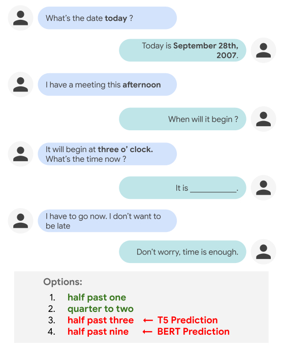
Take, for example, the following audio, which was synthesized from a regular NAT model that takes only phonemes as input:

In comparison, the audio synthesized from PnG NAT on the same input text includes an additional pause that makes the meaning more clear.

The input text to both models is, “To cancel the payment, press one; or to continue, two.” Notice the different pause lengths before the ending “two” in the two versions. The word “two” in the version output by the regular NAT model could be confused for “too”. Because “too” and “two” have identical pronunciation (and thus the same phoneme representation), the regular NAT model does not understand which of the two is appropriate, and assumes it to be the word that more frequently follows a comma, “too”. In contrast, the PnG NAT model can more easily tell the difference, because it takes graphemes in addition to phonemes as input, and thus makes more appropriate pause.

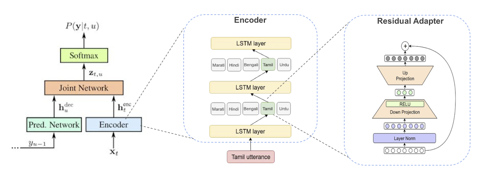
The PnG NAT model integrates the pre-trained PnG BERT model as the encoder to the NAT model. The hidden representations output from the encoder are used by NAT to predict the duration of each phoneme, and are then upsampled to match the length of the audio spectrogram, as outlined above. In the final step, a non-attentive decoder converts the upsampled hidden representations into audio speech spectrograms, which are finally converted into audio waveforms by a neural vocoder.

PnG BERT and the pre-training objectives. Yellow boxes represent phonemes, and pink boxes represent graphemes.
PnG NAT: PnG BERT replaces the original encoder in the NAT model. The random masking for the Masked Language Model (MLM) pre-training is removed.

To recreate Steve Gleason’s voice, we first trained a PnG NAT model with recordings from 31 professional speakers, and then fine-tuned it with 30 minutes of Gleason’s recordings. Because these latter recordings were made after he was diagnosed with ALS, they exhibit signs of slurring. The fine tuned model was able to synthesize speech that sounds very similar to these recordings. However, because the symptoms of ALS were already present in Gleason’s speech, they exhibited some similar disfluencies.

To mitigate this, we leveraged the phoneme duration control of NAT as well as the model trained with professional speakers. We first predicted the durations of each phoneme for both a professional speaker and for Gleason, and then used the geometric mean of the two durations for each phoneme to guide the NAT output. As a result, the model is able to speak in Gleason’s voice, but more fluently than in the original recordings.

Here is the full version of the synthesized Lou Gehrig speech in Gleason’s voice:

Besides recreating voices for people with ALS, PnG NAT is also powering voices for a variety of customers through Google Cloud Custom Voice.

Project Euphonia
Of the millions of people around the world who have neurologic conditions that may impact their speech, such as ALS, cerebral palsy or Down syndrome, many may find it difficult to be understood, which can make face-to-face communication challenging. Using voice-activated technologies can be frustrating too, as they don’t always work reliably. Project Euphonia is a Google Research initiative focused on helping people with impaired speech be better understood. The team is researching ways to improve speech recognition for individuals with speech impairments (see recent blog post and segment in TODAY show), as well as customized text-to-speech technology (see Age of AI documentary featuring former NFL player Tim Shaw).

Acknowledgements
Many people across Google Research, Google Cloud and Consumer Apps, and Google Accessibility teams contributed to this project and the event, including Michael Brenner, Bob MacDonald, Heiga Zen, Yu Zhang, Jonathan Shen, Isaac Elias‎, Yonghui Wu, Anne Keck, Danielle Notaro, Kevin Hogan, Zack Kaplan, KR Liu, Kyndra Price, Zoe Ortiz.

Source: Google AI Blog


Two New Datasets for Conversational NLP: TimeDial and Disfl-QA

A key challenge in natural language processing (NLP) is building conversational agents that can understand and reason about different language phenomena that are unique to realistic speech. For example, because people do not always premeditate exactly what they are going to say, a natural conversation often includes interruptions to speech, called disfluencies. Such disfluencies can be simple (like interjections, repetitions, restarts, or corrections), which simply break the continuity of a sentence, or more complex semantic disfluencies, in which the underlying meaning of a phrase changes. In addition, understanding a conversation also often requires knowledge of temporal relationships, like whether an event precedes or follows another. However, conversational agents built on today’s NLP models often struggle when confronted with temporal relationships or with disfluencies, and progress on improving their performance has been slow. This is due, in part, to a lack of datasets that involve such interesting conversational and speech phenomena.

To stir interest in this direction within the research community, we are excited to introduce TimeDial, for temporal commonsense reasoning in dialog, and Disfl-QA, which focuses on contextual disfluencies. TimeDial presents a new multiple choice span filling task targeted for temporal understanding, with an annotated test set of over ~1.1k dialogs. Disfl-QA is the first dataset containing contextual disfluencies in an information seeking setting, namely question answering over Wikipedia passages, with ~12k human annotated disfluent questions. These benchmark datasets are the first of their kind and show a significant gap between human performance and current state of the art NLP models.

TimeDial
While people can effortlessly reason about everyday temporal concepts, such as duration, frequency, or relative ordering of events in a dialog, such tasks can be challenging for conversational agents. For example, current NLP models often make a poor selection when tasked with filling in a blank (as shown below) that assumes a basic level of world knowledge for reasoning, or that requires understanding explicit and implicit inter-dependencies between temporal concepts across conversational turns.

It is easy for a person to judge that “half past one” and “quarter to two” are more plausible options to fill in the blank than “half past three” and “half past nine”. However, performing such temporal reasoning in the context of a dialog is not trivial for NLP models, as it requires appealing to world knowledge (i.e., knowing that the participants are not yet late for the meeting) and understanding the temporal relationship between events (“half past one” is before “three o’clock”, while “half past three” is after it). Indeed, current state-of-the-art models like T5 and BERT end up picking the wrong answers — “half past three” (T5) and “half past nine” (BERT).

The TimeDial benchmark dataset (derived from the DailyDialog multi-turn dialog corpus) measures models’ temporal commonsense reasoning abilities within a dialog context. Each of the ~1.5k dialogs in the dataset is presented in a multiple choice setup, in which one temporal span is masked out and the model is asked to find all correct answers from a list of four options to fill in the blank.

In our experiments we found that while people can easily answer these multiple choice questions (at 97.8% accuracy), state-of-the-art pre-trained language models still struggle on this challenge set. We experiment across three different modeling paradigms: (i) classification over the provided 4 options using BERT, (ii) mask filling for the masked span in the dialog using BERT-MLM, (iii) generative methods using T5. We observe that all the models struggle on this challenge set, with the best variant only scoring 73%.

Model   2-best Accuracy
Human   97.8%
BERT - Classification   50.0%
BERT - Mask Filling   68.5%
T5 - Generation   73.0%

Qualitative error analyses show that the pre-trained language models often rely on shallow, spurious features (particularly text matching), instead of truly doing reasoning over the context. It is likely that building NLP models capable of performing the kind of temporal commonsense reasoning needed for TimeDial requires rethinking how temporal objects are represented within general text representations.

Disfl-QA
As disfluency is inherently a speech phenomenon, it is most commonly found in text output from speech recognition systems. Understanding such disfluent text is key to building conversational agents that understand human speech. Unfortunately, research in the NLP and speech community has been impeded by the lack of curated datasets containing such disfluencies, and the datasets that are available, like Switchboard, are limited in scale and complexity. As a result, it’s difficult to stress test NLP models in the presence of disfluencies.

Disfluency   Example
Interjection   When is, uh, Easter this year?
Repetition   When is EasEaster this year?
Correction   When is Lent, I mean Easter, this year?
Restart   How much, no wait, when is Easter this year?
Different kinds of disfluencies. The reparandum (words intended to be corrected or ignored; in red), interregnum (optional discourse cues; in grey) and repair (the corrected words; in blue).

Disfl-QA is the first dataset containing contextual disfluencies in an information seeking setting, namely question answering over Wikipedia passages from SQuAD. Disfl-QA is a targeted dataset for disfluencies, in which all questions (~12k) contain disfluencies, making for a much larger disfluent test set than prior datasets. Over 90% of the disfluencies in Disfl-QA are corrections or restarts, making it a much more difficult test set for disfluency correction. In addition, compared to earlier disfluency datasets, it contains a wider variety of semantic distractors, i.e., distractors that carry semantic meaning as opposed to simpler speech disfluencies. 

Passage: …The Normans (Norman: Nourmands; French: Normands; Latin: Normanni) were the people who in the 10th and 11th centuries gave their name to Normandy, a region in France. They were descended from Norse ("Norman" comes from "Norseman") raiders and pirates from Denmark, Iceland and Norway who, under their leader Rollo, …
Q1:   In what country is Normandy located? France ✓
DQ1:   In what country is Norse found no wait Normandy not Norse? Denmark X
Q2:   When were the Normans in Normandy? 10th and 11th centuries ✓
DQ2:   From which countries no tell me when were the Normans in Normandy? Denmark, Iceland and Norway X
A passage and questions (Qi) from SQuAD dataset, along with their disfluent versions (DQi), consisting of semantic distractors (like “Norse” and “from which countries”) and predictions from a T5 model.

Here, the first question (Q1) is seeking an answer about the location of Normandy. In the disfluent version (DQ1) Norse is mentioned before the question is corrected. The presence of this correctional disfluency confuses the QA model, which tends to rely on shallow textual cues from the question for making predictions.

Disfl-QA also includes newer phenomena, such as coreference (expression referring to the same entity) between the reparandum and the repair.

SQuAD  Disfl-QA
Who does BSkyB have an operating license from?  Who removed [BSkyB’s] operating license, no scratch that, who do [they] have [their] operating license from?

Experiments show that the performance of existing state-of-the-art language model–based question answering systems degrades significantly when tested on Disfl-QA and heuristic disfluencies (presented in the paper) in a zero-shot setting.

Dataset   F1
SQuAD   89.59
Heuristics   65.27 (-24.32)
Disfl-QA   61.64 (-27.95)

We show that data augmentation methods partially recover the loss in performance and also demonstrate the efficacy of using human-annotated training data for fine-tuning. We argue that researchers need large-scale disfluency datasets in order for NLP models to be robust to disfluencies.

Conclusion
Understanding language phenomena that are unique to human speech, like disfluencies and temporal reasoning, among others, is a key ingredient for enabling more natural human–machine communication in the near future. With TimeDial and Disfl-QA, we aim to fill a major research gap by providing these datasets as testbeds for NLP models, in order to evaluate their robustness to ubiquitous phenomena across different tasks. It is our hope that the broader NLP community will devise generalized few-shot or zero-shot approaches to effectively handle these phenomena, without requiring task-specific human-annotated training datasets, constructed specifically for these challenges.

Acknowledgments
The TimeDial work has been a team effort involving Lianhui Qi, Luheng He, Yenjin Choi, Manaal Faruqui and the authors. The Disfl-QA work has been a collaboration involving Jiacheng Xu, Diyi Yang, Manaal Faruqui.

Source: Google AI Blog


FRILL: On-Device Speech Representations using TensorFlow-Lite

Representation learning is a machine learning (ML) method that trains a model to identify salient features that can be applied to a variety of downstream tasks, ranging from natural language processing (e.g., BERT and ALBERT) to image analysis and classification (e.g., Inception layers and SimCLR). Last year, we introduced a benchmark for comparing speech representations and a new, generally-useful speech representation model (TRILL). TRILL is based on temporal proximity, and tries to map speech that occurs close together in time to a lower-dimensional embedding that captures temporal proximity in the embedding space. Since its release, the research community has used TRILL on a diverse set of tasks, such as age classification, video thumbnail selection, and language identification. However, despite achieving state-of-the-art performance, TRILL and other neural network-based approaches require more memory and take longer to compute than signal processing operations that deal with simple features, like loudness, average energy, pitch, etc.

In our recent paper "FRILL: A Non-Semantic Speech Embedding for Mobile Devices", to appear at Interspeech 2021, we create a new model that is 40% the size of TRILL and and a feature set that can be computed over 32x faster on mobile phone, with an average decrease in accuracy of less than 2%. This marks an important step towards fully on-device applications of speech ML models, which will lead to better personalization, improved user experiences and greater privacy, an important aspect of developing AI responsibly. We release the code to create FRILL on github, and a pre-trained FRILL model on TensorFlow Hub.

FRILL: Smaller, Faster TRILL
The TRILL architecture is based on a modified version of ResNet50, an architecture that is computationally taxing for constrained hardware, like mobile phones or smart home devices. On the other hand, architectures like MobileNetV3 have been designed with hardware-aware AutoML to perform well on mobile devices. To take advantage of this, we leverage knowledge distillation to combine the benefits of MobileNetV3’s performance with TRILL’s representations.

In the distillation process, the smaller model (i.e., the "student") tries to match the output of the larger model ("teacher") on the AudioSet dataset. Whereas the original TRILL model learned its weights by optimizing a self-supervised loss that clustered audio segments close in time, the student model learns its weights through a fully-supervised loss that ignores temporal matching and instead tries to match TRILL outputs on the training data. The fully-supervised learning signal is often stronger than self-supervision, and allows us to train more quickly.

Knowledge distillation for non-semantic speech embeddings. The dashed line shows the student model output. The "teacher network" is the TRILL network, where "Layer 19" was the best-performing internal representation. The "Student Hyperparameters" on the left are the options explored in this study, the result of which are 144 distinct models. These models were trained with mean-squared error (MSE) to try to match TRILL's Layer 19.

Choosing the Best Student Model
We perform distillation with a variety of student models, each trained with a specific combination of architecture choices (explained below). To measure each student model’s latency, we leverage TensorFlow Lite (TFLite), a framework that enables execution of TensorFlow models on edge devices. Each candidate model is first converted into TFLite’s flatbuffer format for 32-bit floating point inference and then sent to the target device (in this case, a Pixel 1) for benchmarking. These measurements help us to accurately assess the latency versus quality tradeoffs across all student models and to minimize the loss of quality in the conversion process.

Architecture Choices and Optimizations
We explored different neural network architectures and features that balance latency and accuracy — models with fewer parameters are usually smaller and faster, but have less representational power and therefore generate less generally-useful representations. We trained 144 different models across a number of hyperparameters, all based on the MobileNetV3 architecture:

  1. MobileNetV3 size and width: MobileNetV3 was released in different sizes for use in different environments. The size refers to which MobileNetV3 architecture we used. The width, sometimes known as alpha, proportionally decreases or increases the number of filters in each layer. A width of 1.0 corresponds to the number of filters in the original paper.
  2. Global average pooling: MobileNetV3 normally produces a set of two-dimensional feature maps. These are flattened, concatenated, and passed to the bottleneck layer. However, this bottleneck is often still too large to be computed quickly. We reduce the size of the bottleneck layer kernel by taking the global average of all ”pixels” in each output feature map. Our intuition is that the discarded temporal information is less important for learning a non-semantic speech representation due to the fact that relevant aspects of the signal are stable across time.
  3. Bottleneck compression: A significant portion of the student model’s weights are located in the bottleneck layer. To reduce the size of this layer, we apply a compression operator based on singular value decomposition (SVD) that learns a low-rank approximation of the bottleneck weight matrix.
  4. Quantization-aware training: Since the bottleneck layer has most of the model weights, we use quantization-aware training (QAT) to gradually reduce the numerical precision of the bottleneck weights during training. QAT allows the model to adjust to the lower numerical precision during training, instead of potentially causing performance degradation by introducing quantization after training finishes.

Results
We evaluated each of these models on the Non-Semantic Speech Benchmark (NOSS) and two new tasks — a challenging task to detect whether a speaker is wearing a mask and the human-noise subset of the Environment Sound Classification dataset, which includes labels like “coughing” and “sneezing”. After eliminating models that have strictly better alternatives, we are left with eight ”frontier” models on the quality vs. latency curve, which are the models that had no faster and better performance alternatives at a corresponding quality threshold or latency in our batch of 144 models. We plot the latency vs. quality curve of only these "frontier" models below, and we ignore models that are strictly worse.

Embedding quality and latency tradeoff. The x-axis represents the inference latency and the y-axis shows the difference in accuracy from TRILL’s performance, averaged across benchmark datasets.

FRILL is the best performing sub-10ms inference model, with an inference time of 8.5 ms on a Pixel 1 (about 32x faster than TRILL), and is also roughly 40% the size of TRILL. The frontier curve plateaus at about 10ms latency, which means that at low latency, one can achieve much better performance with minimal latency costs, while achieving improved performance at latencies beyond 10ms is more difficult. This supports our choice of experiment hyperparameters. FRILL's per-task performance is shown in the table below.

FRILL TRILL

Size (MB) 38.5 98.1
Latency (ms) 8.5 275.3

Voxceleb1* 45.5 46.8
Voxforge 78.8 84.5
Speech Commands 81.0 81.7
CREMA-D 71.3 65.9
SAVEE 63.3 70.0
Masked Speech 68.0 65.8
ESC-50 HS 87.9 86.4
Accuracy on each of the classification tasks (higher is better).
*Results in our study use a small subset of Voxceleb1 filtered according to internal privacy guidelines. Interested readers can run our study on the full dataset using TensorFlow Datasets and our open-source evaluation code.

Finally, we evaluate the relative contribution of each of our hyperparameters. We find that for our experiments, quantization-aware training, bottleneck compression and global average pooling most reduced the latency of the resulting models. At the same time bottleneck compression most reduced the quality of the resulting model, while pooling reduced the model performance the least. The architecture width parameter was an important factor in reducing the model size, with minimal performance degradation.

Linear regression weight magnitudes for predicting model quality, latency, and size. The weights indicate the expected impact of changing the input hyperparameter. A higher weight magnitude indicates a greater expected impact.

Our work is an important step in bringing the full benefits of speech machine learning research to mobile devices. We also provide our public model, corresponding model card, and evaluation code to help the research community responsibly develop even more applications for on-device speech representation research.

Acknowledgements
We'd like to thank our paper co-authors: Jacob Peplinksi and Shwetak Patel. We'd like to thank Aren Jansen for his technical support on this project, Françoise Beaufays, and Tulsee Doshi for help open sourcing the model, and Google Research, Tokyo for logistical support.

Source: Google AI Blog


Stabilizing Live Speech Translation in Google Translate

The transcription feature in the Google Translate app may be used to create a live, translated transcription for events like meetings and speeches, or simply for a story at the dinner table in a language you don’t understand. In such settings, it is useful for the translated text to be displayed promptly to help keep the reader engaged and in the moment.

However, with early versions of this feature the translated text suffered from multiple real-time revisions, which can be distracting. This was because of the non-monotonic relationship between the source and the translated text, in which words at the end of the source sentence can influence words at the beginning of the translation.

Transcribe (old) — Left: Source transcript as it arrives from speech recognition. Right: Translation that is displayed to the user. The frequent corrections made to the translation interfere with the reading experience.

Today, we are excited to describe some of the technology behind a recently released update to the transcribe feature in the Google Translate app that significantly reduces translation revisions and improves the user experience. The research enabling this is presented in two papers. The first formulates an evaluation framework tailored to live translation and develops methods to reduce instability. The second demonstrates that these methods do very well compared to alternatives, while still retaining the simplicity of the original approach. The resulting model is much more stable and provides a noticeably improved reading experience within Google Translate.

Transcribe (new) — Left: Source transcript as it arrives from speech recognition. Right: Translation that is displayed to the user. At the cost of a small delay, the translation now rarely needs to be corrected.

Evaluating Live Translation
Before attempting to make any improvements, it was important to first understand and quantifiably measure the different aspects of the user experience, with the goal of maximizing quality while minimizing latency and instability. In “Re-translation Strategies For Long Form, Simultaneous, Spoken Language Translation”, we developed an evaluation framework for live-translation that has since guided our research and engineering efforts. This work presents a performance measure using the following metrics:

  • Erasure: Measures the additional reading burden on the user due to instability. It is the number of words that are erased and replaced for every word in the final translation.
  • Lag: Measures the average time that has passed between when a user utters a word and when the word’s translation displayed on the screen becomes stable. Requiring stability avoids rewarding systems that can only manage to be fast due to frequent corrections.
  • BLEU score: Measures the quality of the final translation. Quality differences in intermediate translations are captured by a combination of all metrics.

It is important to recognize the inherent trade-offs between these different aspects of quality. Transcribe enables live-translation by stacking machine translation on top of real-time automatic speech recognition. For each update to the recognized transcript, a fresh translation is generated in real time; several updates can occur each second. This approach placed Transcribe at one extreme of the 3 dimensional quality framework: it exhibited minimal lag and the best quality, but also had high erasure. Understanding this allowed us to work towards finding a better balance.

Stabilizing Re-translation
One straightforward solution to reduce erasure is to decrease the frequency with which translations are updated. Along this line, “streaming translation” models (for example, STACL and MILk) intelligently learn to recognize when sufficient source information has been received to extend the translation safely, so the translation never needs to be changed. In doing so, streaming translation models are able to achieve zero erasure.

The downside with such streaming translation models is that they once again take an extreme position: zero erasure necessitates sacrificing BLEU and lag. Rather than eliminating erasure altogether, a small budget for occasional instability may allow better BLEU and lag. More importantly, streaming translation would require retraining and maintenance of specialized models specifically for live-translation. This precludes the use of streaming translation in some cases, because keeping a lean pipeline is an important consideration for a product like Google Translate that supports 100+ languages.

In our second paper, “Re-translation versus Streaming for Simultaneous Translation”, we show that our original “re-translation” approach to live-translation can be fine-tuned to reduce erasure and achieve a more favorable erasure/lag/BLEU trade-off. Without training any specialized models, we applied a pair of inference-time heuristics to the original machine translation models — masking and biasing.

The end of an on-going translation tends to flicker because it is more likely to have dependencies on source words that have yet to arrive. We reduce this by truncating some number of words from the translation until the end of the source sentence has been observed. This masking process thus trades latency for stability, without affecting quality. This is very similar to delay-based strategies used in streaming methods such as Wait-k, but applied only during inference and not during training.

Neural machine translation often “see-saws” between equally good translations, causing unnecessary erasure. We improve stability by biasing the output towards what we have already shown the user. On top of reducing erasure, biasing also tends to reduce lag by stabilizing translations earlier. Biasing interacts nicely with masking, as masking words that are likely to be unstable also prevents the model from biasing toward them. However, this process does need to be tuned carefully, as a high bias, along with insufficient masking, may have a negative impact on quality.

The combination of masking and biasing, produces a re-translation system with high quality and low latency, while virtually eliminating erasure. The table below shows how the metrics react to the heuristics we introduced and how they compare to the other systems discussed above. The graph demonstrates that even with a very small erasure budget, re-translation surpasses zero-flicker streaming translation systems (MILk and Wait-k) trained specifically for live-translation.

System     BLEU     Lag (s)     Erasure
Re-translation (old)     20.4     4.1     2.1
+ Stabilization (new)     20.2     4.1     0.1
Evaluation of re-translation on IWSLT test 2018 Engish-German (TED talks) with and without the inference-time stabilization heuristics of masking and biasing. Stabilization drastically reduces erasure. Translation quality, measured in BLEU, is very slightly impacted due to biasing. Despite masking, the effective lag remains the same because the translation stabilizes sooner.
Comparison of re-translation with stabilization and specialized streaming models (Wait-k and MILk) on WMT 14 English-German. The BLEU-lag trade-off curve for re-translation is obtained via different combinations of bias and masking while maintaining an erasure budget of less than 2 words erased for every 10 generated. Re-translation offers better BLEU / lag trade-offs than streaming models which cannot make corrections and require specialized training for each trade-off point.

Conclusion
The solution outlined above returns a decent translation very quickly, while allowing it to be revised as more of the source sentence is spoken. The simple structure of re-translation enables the application of our best speech and translation models with minimal effort. However, reducing erasure is just one part of the story — we are also looking forward to improving the overall speech translation experience through new technology that can reduce lag when the translation is spoken, or that can enable better transcriptions when multiple people are speaking.

Acknowledgements
Thanks to Te I, Dirk Padfield, Pallavi Baljekar, Goerge Foster, Wolfgang Macherey, John Richardson, Kuang-Che Lee, Byran Lin, Jeff Pittman, Sami Iqram, Mengmeng Niu, Macduff Hughes, Chris Kau, Nathan Bain.

Source: Google AI Blog


Audiovisual Speech Enhancement in YouTube Stories

While tremendous efforts are invested in improving the quality of videos taken with smartphone cameras, the quality of audio in videos is often overlooked. For example, the speech of a subject in a video where there are multiple people speaking or where there is high background noise might be muddled, distorted, or difficult to understand. In an effort to address this, two years ago we introduced Looking to Listen, a machine learning (ML) technology that uses both visual and audio cues to isolate the speech of a video’s subject. By training the model on a large-scale collection of online videos, we are able to capture correlations between speech and visual signals such as mouth movements and facial expressions, which can then be used to separate the speech of one person in a video from another, or to separate speech from background sounds. We showed that this technology not only achieves state-of-the-art results in speech separation and enhancement (a noticeable 1.5dB improvement over audio-only models), but in particular can improve the results over audio-only processing when there are multiple people speaking, as the visual cues in the video help determine who is saying what.

We are now happy to make the Looking to Listen technology available to users through a new audiovisual Speech Enhancement feature in YouTube Stories (on iOS), allowing creators to take better selfie videos by automatically enhancing their voices and reducing background noise. Getting this technology into users’ hands was no easy feat. Over the past year, we worked closely with users to learn how they would like to use such a feature, in what scenarios, and what balance of speech and background sounds they would like to have in their videos. We heavily optimized the Looking to Listen model to make it run efficiently on mobile devices, overall reducing the running time from 10x real-time on a desktop when our paper came out, to 0.5x real-time performance on the phone. We also put the technology through extensive testing to verify that it performs consistently across different recording conditions and for people with different appearances and voices.

From Research to Product
Optimizing Looking to Listen to allow fast and robust operation on mobile devices required us to overcome a number of challenges. First, all processing needed to be done on-device within the client app in order to minimize processing time and to preserve the user’s privacy; no audio or video information would be sent to servers for processing. Further, the model needed to co-exist alongside other ML algorithms used in the YouTube app in addition to the resource-consuming video recording itself. Finally, the algorithm needed to run quickly and efficiently on-device while minimizing battery consumption.

The first step in the Looking to Listen pipeline is to isolate thumbnail images that contain the faces of the speakers from the video stream. By leveraging MediaPipe BlazeFace with GPU accelerated inference, this step is now able to be executed in just a few milliseconds. We then switched the model part that processes each thumbnail separately to a lighter weight MobileNet (v2) architecture, which outputs visual features learned for the purpose of speech enhancement, extracted from the face thumbnails in 10 ms per frame. Because the compute time to embed the visual features is short, it can be done while the video is still being recorded. This avoids the need to keep the frames in memory for further processing, thereby reducing the overall memory footprint. Then, after the video finishes recording, the audio and the computed visual features are streamed to the audio-visual speech separation model which produces the isolated and enhanced speech.

We reduced the total number of parameters in the audio-visual model by replacing “regular” 2D convolutions with separable ones (1D in the frequency dimension, followed by 1D in the time dimension) with fewer filters. We then optimized the model further using TensorFlow Lite — a set of tools that enable running TensorFlow models on mobile devices with low latency and a small binary size. Finally, we reimplemented the model within the Learn2Compress framework in order to take advantage of built-in quantized training and QRNN support.

Our Looking to Listen on-device pipeline for audiovisual speech enhancement

These optimizations and improvements reduced the running time from 10x real-time on a desktop using the original formulation of Looking to Listen, to 0.5x real-time performance using only an iPhone CPU; and brought the model size down from 120MB to 6MB now, which makes it easier to deploy. Since YouTube Stories videos are short — limited to 15 seconds — the result of the video processing is available within a couple of seconds after the recording is finished.

Finally, to avoid processing videos with clean speech (so as to avoid unnecessary computation), we first run our model only on the first two seconds of the video, then compare the speech-enhanced output to the original input audio. If there is sufficient difference (meaning the model cleaned up the speech), then we enhance the speech throughout the rest of the video.

Researching User Needs
Early versions of Looking to Listen were designed to entirely isolate speech from the background noise. In a user study conducted together with YouTube, we found that users prefer to leave in some of the background sounds to give context and to retain some the general ambiance of the scene. Based on this user study, we take a linear combination of the original audio and our produced clean speech channel: output_audio = 0.1 x original_audio + 0.9 x speech. The following video presents clean speech combined with different levels of the background sounds in the scene (10% background is the balance we use in practice).

Below are additional examples of the enhanced speech results from the new Speech Enhancement feature in YouTube Stories. We recommend watching the videos with good speakers or headphones.

Fairness Analysis
Another important requirement is that the model be fair and inclusive. It must be able to handle different types of voices, languages and accents, as well as different visual appearances. To this end, we conducted a series of tests exploring the performance of the model with respect to various visual and speech/auditory attributes: the speaker’s age, skin tone, spoken language, voice pitch, visibility of the speaker’s face (% of video in which the speaker is in frame), head pose throughout the video, facial hair, presence of glasses, and the level of background noise in the (input) video.

For each of the above visual/auditory attributes, we ran our model on segments from our evaluation set (separate from the training set) and measured the speech enhancement accuracy, broken down according to the different attribute values. Results for some of the attributes are summarized in the following plots. Each data point in the plots represents hundreds (in most cases thousands) of videos fitting the criteria.

Speech enhancement quality (signal-to-distortion ratio, SDR, in dB) for different spoken languages, sorted alphabetically. The average SDR was 7.89 dB with a standard deviation of 0.42 dB — deviation that for human listeners is considered hard to notice.
Left: Speech enhancement quality as a function of the speaker’s voice pitch. The fundamental voice frequency (pitch) of an adult male typically ranges from 85 to 180 Hz, and that of an adult female ranges from 165 to 255 Hz. Right: speech enhancement quality as a function of the speaker’s predicted age.
As our method utilizes facial cues and mouth movements to isolate the speech, we tested whether facial hair (e.g., a moustache, beard) may obstruct those visual cues and affect the method’s performance. Our evaluations show that the quality of speech enhancement is maintained well also in the presence of facial hair.

Using the Feature
YouTube creators who are eligible for YouTube Stories creation may record a video on iOS, and select “Enhance speech” from the volume controls editing tool. This will immediately apply speech enhancement to the audio track and will play back the enhanced speech in a loop. It is then possible to toggle the feature on and off multiple times to compare the enhanced speech with the original audio.

In parallel to this new feature in YouTube, we are also exploring additional venues for this technology. More to come later this year — stay tuned!

Acknowledgements
This feature is a collaboration across multiple teams at Google. Key contributors include: from Research-IL: Oran Lang; from VisCAM: Ariel Ephrat, Mike Krainin, JD Velasquez, Inbar Mosseri, Michael Rubinstein; from Learn2Compress: Arun Kandoor; from MediaPipe: Buck Bourdon, Matsvei Zhdanovich, Matthias Grundmann; from YouTube: Andy Poes, Vadim Lavrusik, Aaron La Lau, Willi Geiger, Simona De Rosa, and Tomer Margolin.

Source: Google AI Blog


Improving Speech Representations and Personalized Models Using Self-Supervision


There are many tasks within speech processing that are easier to solve by having large amounts of data. For example automatic speech recognition (ASR) translates spoken audio into text. In contrast, "non-semantic" tasks focus on the aspects of human speech other than its meaning, encompassing "paralinguistic" tasks, like speech emotion recognition, as well as other kinds of tasks, such as speaker identification, language identification, and certain kinds of voice-based medical diagnoses. In training systems to accomplish these tasks, one common approach is to utilize the largest datasets possible to help ensure good results. However, machine learning techniques that directly rely on massive datasets are often less successful when trained on small datasets.

One way to bridge the performance gap between large and small datasets is to train a representation model on a large dataset, then transfer it to a setting with less data. Representations can improve performance in two ways: they can make it possible to train small models by transforming high-dimensional data (like images and audio) to a lower dimension, and the representation model can also be used as pre-training. In addition, if the representation model is small enough to be run or trained on-device, it can improve performance in a privacy-preserving way by giving users the benefits of a personalized model where the raw data never leaves their device. While representation learning is commonly used in the text domain (e.g. BERT and ALBERT) and in the images domain (e.g. Inception layers and SimCLR), such approaches are underutilized in the speech domain.
Bottom:A large speech dataset is used to train a model, which is then rolled out to other environments. Top Left: On-device personalization — personalized, on-device models combine security and privacy. Top Middle: Small model on embeddings — general-use representations transform high-dimensional, few-example datasets to a lower dimension without sacrificing accuracy; smaller models train faster and are regularized. Top Right: Full model fine-tuning — large datasets can use the embedding model as pre-training to improve performance
Unambiguously improving generally-useful representations, for non-semantic speech tasks in particular, is difficult without a standard benchmark to compare "speech representation usefulness." While the T5 framework systematically evaluates text embeddings and the Visual Task Adaptation Benchmark (VTAB) standardizes image embedding evaluation, both leading to progress in representation learning in those respective fields, there has been no such benchmark for non-semantic speech embeddings.

In "Towards Learning a Universal Non-Semantic Representation of Speech", we make three contributions to representation learning for speech-related applications. First, we present a NOn-Semantic Speech (NOSS) benchmark for comparing speech representations, which includes diverse datasets and benchmark tasks, such as speech emotion recognition, language identification, and speaker identification. These datasets are available in the "audio" section of TensorFlow Datasets. Second, we create and open-source TRIpLet Loss network (TRILL), a new model that is small enough to be executed and fine-tuned on-device, while still outperforming other representations. Third, we perform a large-scale study comparing different representations, and open-source the code used to compute the performance on new representations.

A New Benchmark for Speech Embeddings
For a benchmark to usefully guide model development, it must contain tasks that ought to have similar solutions and exclude those that are significantly different. Previous work either dealt with the variety of possible speech-based tasks independently, or lumped semantic and non-semantic tasks together. Our work improves performance on non-semantic speech tasks, in part, by focusing on neural network architectures that perform well specifically on this subset of speech tasks.

The tasks were selected for the NOSS benchmark on the basis of their 1) diversity — they need to cover a range of use-cases; 2) complexity — they should be challenging; and 3) availability, with particular emphasis on those tasks that are open-source. We combined six datasets of different sizes and tasks.
Datasets for downstream benchmark tasks. *VoxCeleb results in our study were computed using a subset of the dataset that was filtered according to internal policy.
We also introduce three additional intra-speaker tasks to test performance in the personalization scenario. In some datasets with k speakers, we can create k different tasks consisting of training and testing on just a single speaker. Overall performance is averaged across speakers. These three additional intra-speaker tasks measure the ability of an embedding to adapt to a particular speaker, as would be necessary for personalized, on-device models, which are becoming more important as computation moves to smart phones and the internet of things.

To help enable researchers to compare speech embeddings, we’ve added the six datasets in our benchmark to TensorFlow Datasets (in the "audio" section) and open sourced the evaluation framework.

TRILL: A New State of the Art in Non-semantic Speech Classification
Learning an embedding from one dataset and applying it to other tasks is not as common in speech as in other modalities. However, transfer learning, the more general technique of using data from one task to help another (not necessarily with embeddings), has some compelling applications, such as personalizing speech recognizers and voice imitation text-to-speech from few samples. There have been many previously proposed representations of speech, but most of these have been trained on a smaller and less diverse data, have been tested primarily on speech recognition, or both.

To create a data-derived representation of speech that was useful across environments and tasks, we started with AudioSet, a large and diverse dataset that includes about 2500 hours of speech. We then trained an embedding model on a simple, self-supervised criteria derived from previous work on metric learning — embeddings from the same audio should be closer in embedding space than embeddings from different audio. Like BERT and the other text embeddings, the self-supervised loss function doesn't require labels and only relies on the structure of the data itself. This form of self-supervision is the most appropriate for non-semantic speech, since non-semantic phenomena are more stable in time than ASR and other sub-second speech characteristics. This simple, self-supervised criteria captures a large number of acoustic properties that are leveraged in downstream tasks.
TRILL loss: Embeddings from the same audio are closer in embedding space than embeddings from different audio.
TRILL architecture is based on MobileNet, making it fast enough to run on mobile devices. To achieve high accuracy on this small architecture, we distilled the embedding from a larger ResNet50 model without performance degradation.

Benchmark Results
We compared the performance of TRILL against other deep learning representations that are not focused on speech recognition and were trained on similarly diverse datasets. In addition, we compared TRILL to the popular OpenSMILE feature extractor, which uses pre-deep learning techniques (e.g., a fourier transform coefficients, "pitch tracking" using a time-series of pitch measurements, etc.), and randomly initialized networks, which have been shown to be strong baselines. To aggregate the performance across tasks that have different performance characteristics, we first train a small number of simple models, for a given task and embedding. The best result is chosen. Then, to understand the effect that a particular embedding has across all tasks, we calculate a linear regression on the observed accuracies, with both the model and task as the explanatory variables. The effect a model has on the accuracy is the coefficient associated with the model in the regression. For a given task, when changing from one model to another, the resulting change in accuracy is expected to be the difference in y-values in the figure below.
Effect of model on accuracy.
TRILL outperforms the other representations in our study. Factors that contribute to TRILL's success are the diversity of the training dataset, the large context window of the network, and the generality of the TRILL training loss that broadly preserves acoustic characteristics instead of prematurely focusing on certain aspects. Note that representations from intermediate network layers are often more generally useful. The intermediate representations are larger, have finer temporal granularity, and in the case of the classification networks they retain more general information that isn't as specific to the classes on which they were trained.

Another benefit of a generally-useful model is that it can be used to initialize a model on a new task. When the sample size of a new task is small, fine-tuning an existing model may lead to better results than training the model from scratch. We achieved a new state-of-the-art result on three out of six benchmark tasks using this technique, despite doing no dataset-specific hyperparameter tuning.

To compare our new representation, we also tested it on the mask sub-challenge of the Interspeech 2020 Computational Paralinguistics Challenge (ComParE). In this challenge, models must predict whether a speaker is wearing a mask, which would affect their speech. The mask effects are sometimes subtle, and audio clips are only one second long. A linear model on TRILL outperformed the best baseline model, which was a fusion of many models on different kinds of features including traditional spectral and deep-learned features.

Summary
The code to evaluate NOSS is available on GitHub, the datasets are on TensorFlow Datasets, and the TRILL models are available on AI Hub.

The NOn-Semantic Speech benchmark helps researchers create speech embeddings that are useful in a wide range of contexts, including for personalization and small-dataset problems. We provide the TRILL model to the research community as a baseline embedding to surpass.

Acknowledgements
The core team behind this work includes Joel Shor, Aren Jansen, Ronnie Maor, Oran Lang, Omry Tuval, Felix de Chaumont Quitry, Marco Tagliasacchi, Ira Shavitt, Dotan Emanuel, and Yinnon Haviv. We'd also like to thank Avinatan Hassidim and Yossi Matias for technical guidance.

Source: Google AI Blog


Improving Audio Quality in Duo with WaveNetEQ


Online calls have become an everyday part of life for millions of people by helping to streamline their work and connect them to loved ones. To transmit a call across the internet, the data from calls are split into short chunks, called packets. These packets make their way over the network from the sender to the receiver where they are reassembled to make continuous streams of video and audio. However, packets often arrive at the other end in the wrong order or at the wrong time, an issue generally referred to as jitter, and sometimes individual packets can be lost entirely. Issues such as these lead to lower call quality, since the receiver has to try and fill in the gaps, and are a pervasive problem for both audio and video transmission. For example, 99% of Google Duo calls need to deal with packet losses, excessive jitter or network delays. Of those calls, 20% lose more than 3% of the total audio duration due to network issues, and 10% of calls lose more than 8%.
Simplified diagram of network problems leading to packet loss, which needs to be counteracted by the receiver to allow reliable real-time communication.
In order to ensure reliable real-time communication, it is necessary to deal with packets that are missing when the receiver needs them. Specifically, if new audio is not provided continuously, glitches and gaps will be audible, but repeating the same audio over and over is not an ideal solution, as it produces artifacts and reduces the overall quality of the call. The process of dealing with the missing packets is called packet loss concealment (PLC). The receiver’s PLC module is responsible for creating audio (or video) to fill in the gaps created by packet losses, excessive jitter or temporary network glitches, all three of which result in an absence of data.

To address these audio issues, we present WaveNetEQ, a new PLC system now being used in Duo. WaveNetEQ is a generative model, based on DeepMind’s WaveRNN technology, that is trained using a large corpus of speech data to realistically continue short speech segments enabling it to fully synthesize the raw waveform of missing speech. Because Duo calls are end-to-end encrypted, all processing needs to be done on-device. The WaveNetEQ model is fast enough to run on a phone, while still providing state-of-the-art audio quality and more natural sounding PLC than other systems currently in use.

A New PLC System for Duo
Like many other web-based communication systems, Duo is based on the WebRTC open source project. To conceal the effects of packet loss, WebRTC’s NetEQ component uses signal processing methods, which analyze the speech and produce a smooth continuation that works very well for small losses (20ms or less), but does not sound good when the number of missing packets leads to gaps of 60ms or more. In those latter cases the speech becomes robotic and repetitive, a characteristic sound that is unfortunately familiar to many internet voice callers.

To better manage packet loss, we replace the NetEQ PLC component with a modified version of WaveRNN, a recurrent neural network model for speech synthesis consisting of two parts, an autoregressive network and a conditioning network. The autoregressive network is responsible for the continuity of the signal and provides the short-term and mid-term structure for the speech by having each generated sample depend on the network’s previous outputs. The conditioning network influences the autoregressive network to produce audio that is consistent with the more slowly-moving input features.

However, WaveRNN, like its predecessor WaveNet, was created with the text-to-speech (TTS) application in mind. As a TTS model, WaveRNN is supplied with the information of what it is supposed to say and how to say it. The conditioning network directly receives this information as input in form of the phonemes that make up the words and additional prosody features (i.e., all non-text information like intonation or pitch). In a way, the conditioning network can “see into the future” and then steer the autoregressive network towards the right waveforms to match it. In the case of a PLC system and real-time communication, this context is not provided.

For a functional PLC system, one must both extract contextual information from the current speech (i.e., the past), and generate a plausible sound to continue it. Our solution, WaveNetEQ, does both at the same time, using the autoregressive network to provide the audio continuation during a packet loss event, and the conditioning network to model long term features, like voice characteristics. The spectrogram of the past audio signal is used as input for the conditioning network, which extracts limited information about the prosody and textual content. This condensed information is fed to the autoregressive network, which combines it with the audio of the recent past to predict the next sample in the waveform domain.

This differs slightly from the procedure that was followed during training of the WaveNetEQ model, where the autoregressive network receives the actual sample present in the training data as input for the next step, rather than using the last sample it produced. This process, called teacher forcing, assures that the model learns valuable information, even at an early stage of training when its predictions are still of low quality. Once the model is fully trained and put to use in an audio or video call, teacher forcing is only used to "warm up" the model for the first sample, and after that its own output is passed back as input for the next step.
WaveNetEQ architecture. During inference, we "warm up" the autoregressive network by teacher forcing with the most recent audio. Afterwards, the model is supplied with its own output as input for the next step. A MEL spectrogram from a longer audio part is used as input for the conditioning network.
The model is applied to the audio data in Duo's jitter buffer. Once the real audio continues after a packet loss event, we seamlessly merge the synthetic and real audio stream. In order to find the best alignment between the two signals, the model generates slightly more output than is required and then cross-fades from one to the other. This makes the transition smooth and avoids noticeable noise.
Simulation of PLC events on audio over a moving span of 60 ms. The blue line represents the real audio signal, including past and future parts of the PLC event. At each timestep the orange line represents the synthetic audio WaveNetEQ would predict if the audio were to cut out at the vertical grey line.
60 ms Packet Loss
NetEQ
WaveNetEQ
NetEQ
WaveNetEQ

120 ms Packet Loss
NetEQ
WaveNetEQ
NetEQ
WaveNetEQ
Audio clips: Comparison of WebRTC’s default PLC system, NetEQ, with our model, WaveNetEQ. Audio clips were taken from LibriTTS and 10% of the audio was dropped in 60 or 120 ms chunks and then filled in by the PLC systems.
Ensuring Robustness
One important factor during PLC is the ability of the network to adapt to variable input signals, including different speakers or changes in background noise. In order to ensure the robustness of the model across a wide range of users, we trained WaveNetEQ on a speech dataset that contains over 100 speakers in 48 different languages, which allows the model to learn the characteristics of human speech in general, instead of the properties of a specific language. To ensure WaveNetEQ is able to deal with noisy environments, such as answering your phone in the train station or in the cafeteria, we augment the data by mixing it with a wide variety of background noises.

While our model learns how to plausibly continue speech, this is only true on a short scale — it can finish a syllable but does not predict words, per se. Instead, for longer packet losses we gradually fade out until the model only produces silence after 120 milliseconds. To further ensure that the model is not generating false syllables, we evaluated samples from WaveNetEQ and NetEQ using the Google Cloud Speech-to-Text API and found no significant difference in the word error rate, i.e., how many mistakes were made transcribing the spoken text.

We have been experimenting with WaveNetEQ in Duo, where the feature has demonstrated a positive impact on call quality and user experience. WaveNetEQ is already available in all Duo calls on Pixel 4 phones and is now being rolled out to additional models.

Acknowledgements
The core team includes Alessio Bazzica, Niklas Blum, Lennart Kolmodin, Henrik Lundin, Alex Narest, Olga Sharonova from Google and Tom Walters from DeepMind. We would also like to thank Martin Bruse (Google), Norman Casagrande, Ray Smith, Chenjie Gu and Erich Elsen (DeepMind) for their contributions.

Source: Google AI Blog


Large-Scale Multilingual Speech Recognition with a Streaming End-to-End Model


Google's mission is not just to organize the world's information but to make it universally accessible, which means ensuring that our products work in as many of the world's languages as possible. When it comes to understanding human speech, which is a core capability of the Google Assistant, extending to more languages poses a challenge: high-quality automatic speech recognition (ASR) systems require large amounts of audio and text data — even more so as data-hungry neural models continue to revolutionize the field. Yet many languages have little data available.

We wondered how we could keep the quality of speech recognition high for speakers of data-scarce languages. A key insight from the research community was that much of the "knowledge" a neural network learns from audio data of a data-rich language is re-usable by data-scarce languages; we don't need to learn everything from scratch. This led us to study multilingual speech recognition, in which a single model learns to transcribe multiple languages.

In “Large-Scale Multilingual Speech Recognition with a Streaming End-to-End Model”, published at Interspeech 2019, we present an end-to-end (E2E) system trained as a single model, which allows for real-time multilingual speech recognition. Using nine Indian languages, we demonstrated a dramatic improvement in the ASR quality on several data-scarce languages, while still improving performance for the data-rich languages.

India: A Land of Languages
For this study, we focused on India, an inherently multilingual society where there are more than thirty languages with at least a million native speakers. Many of these languages overlap in acoustic and lexical content due to the geographic proximity of the native speakers and shared cultural history. Additionally, many Indians are bilingual or trilingual, making the use of multiple languages within a conversation a common phenomenon, and a natural case for training a single multilingual model. In this work, we combined nine primary Indian languages, namely Hindi, Marathi, Urdu, Bengali, Tamil, Telugu, Kannada, Malayalam and Gujarati.

A Low-latency All-neural Multilingual Model
Traditional ASR systems contain separate components for acoustic, pronunciation, and language models. While there have been attempts to make some or all of the traditional ASR components multilingual [1,2,3,4], this approach can be complex and difficult to scale. E2E ASR models combine all three components into a single neural network and promise scalability and ease of parameter sharing. Recent works have extended E2E models to be multilingual [1,2], but they did not address the need for real-time speech recognition, a key requirement for applications such as the Assistant, Voice Search and GBoard dictation. For this, we turned to recent research at Google that used a Recurrent Neural Network Transducer (RNN-T) model to achieve streaming E2E ASR. The RNN-T system outputs words one character at a time, just as if someone was typing in real time, however this was not multilingual. We built upon this architecture to develop a low-latency model for multilingual speech recognition.
[Left] A traditional monolingual speech recognizer comprising of Acoustic, Pronunciation and Language Models for each language. [Middle] A traditional multilingual speech recognizer where the Acoustic and Pronunciation model is multilingual, while the Language model is language-specific. [Right] An E2E multilingual speech recognizer where the Acoustic, Pronunciation and Language Model is combined into a single multilingual model.
Large-Scale Data Challenges
Using large-scale, real-world data for training a multilingual model is complicated by data imbalance. Given the steep skew in the distribution of speakers across the languages and speech product maturity, it is not surprising to have varying amounts of transcribed data available per language. As a result, a multilingual model can tend to be more influenced by languages that are over-represented in the training set. This bias is more prominent in an E2E model, which unlike a traditional ASR system, does not have access to additional in-language text data and learns lexical characteristics of the languages solely from the audio training data.
Histogram of training data for the nine languages showing the steep skew in the data available.
We addressed this issue with a few architectural modifications. First, we provided an extra language identifier input, which is an external signal derived from the language locale of the training data; i.e. the language preference set in an individual’s phone. This signal is combined with the audio input as a one-hot feature vector. We hypothesize that the model is able to use the language vector not only to disambiguate the language but also to learn separate features for separate languages, as needed, which helped with data imbalance.

Building on the idea of language-specific representations within the global model, we further augmented the network architecture by allocating extra parameters per language in the form of residual adapter modules. Adapters helped fine-tune a global model on each language while maintaining parameter efficiency of a single global model, and in turn, improved performance.
[Left] Multilingual RNN-T architecture with a language identifier. [Middle] Residual adapters inside the encoder. For a Tamil utterance, only the Tamil adapters are applied to each activation. [Right] Architecture details of the Residual Adapter modules. For more details please see our paper.
Putting all of these elements together, our multilingual model outperforms all the single-language recognizers, with especially large improvements in data-scarce languages like Kannada and Urdu. Moreover, since it is a streaming E2E model, it simplifies training and serving, and is also usable in low-latency applications like the Assistant. Building on this result, we hope to continue our research on multilingual ASRs for other language groups, to better assist our growing body of diverse users.

Acknowledgements
We would like to thank the following for their contribution to this research: Tara N. Sainath, Eugene Weinstein, Bo Li, Shubham Toshniwal, Ron Weiss, Bhuvana Ramabhadran, Yonghui Wu, Ankur Bapna, Zhifeng Chen, Seungji Lee, Meysam Bastani, Mikaela Grace, Pedro Moreno, Yanzhang (Ryan) He, Khe Chai Sim.

Source: Google AI Blog