Tag Archives: machine learning

Text Embedding Models Contain Bias. Here’s Why That Matters.

Posted by Ben Packer, Yoni Halpern, Mario Guajardo-Céspedes & Margaret Mitchell (Google AI)

As Machine Learning practitioners, when faced with a task, we usually select or train a model primarily based on how well it performs on that task. For example, say we're building a system to classify whether a movie review is positive or negative. We take 5 different models and see how well each performs this task:

Figure 1: Model performances on a task. Which model would you choose?

Normally, we'd simply choose Model C. But what if we found that while Model C performs the best overall, it's also most likely to assign a more positive sentiment to the sentence "The main character is a man" than to the sentence "The main character is a woman"? Would we reconsider?

Bias in Machine Learning Models

Neural network models can be quite powerful, effectively helping to identify patterns and uncover structure in a variety of different tasks, from language translation to pathology to playing games. At the same time, neural models (as well as other kinds of machine learning models) can contain problematic biases in many forms. For example, classifiers trained to detect rude, disrespectful, or unreasonable comments may be more likely to flag the sentence "I am gay" than "I am straight" [1]; face classification models may not perform as well for women of color [2]; speech transcription may have higher error rates for African Americans than White Americans [3].

Many pre-trained machine learning models are widely available for developers to use -- for example, TensorFlow Hub recently launched its platform publicly. It's important that when developers use these models in their applications, they're aware of what biases they contain and how they might manifest in those applications.

Human data encodes human biases by default. Being aware of this is a good start, and the conversation around how to handle it is ongoing. At Google, we are actively researching unintended bias analysis and mitigation strategies because we are committed to making products that work well for everyone. In this post, we'll examine a few text embedding models, suggest some tools for evaluating certain forms of bias, and discuss how these issues matter when building applications.

WEAT scores, a general-purpose measurement tool

Text embedding models convert any input text into an output vector of numbers, and in the process map semantically similar words near each other in the embedding space:

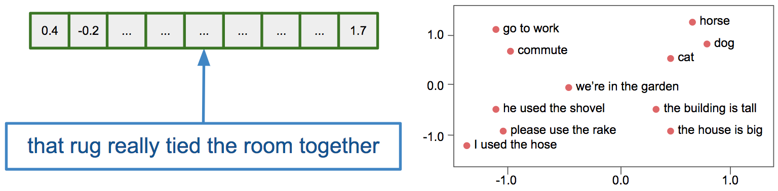
Figure 2: Text embeddings convert any text into a vector of numbers (left). Semantically similar pieces of text are mapped nearby each other in the embedding space (right).

Given a trained text embedding model, we can directly measure the associations the model has between words or phrases. Many of these associations are expected and are helpful for natural language tasks. However, some associations may be problematic or hurtful. For example, the ground-breaking paper by Bolukbasi et al. [4] found that the vector-relationship between "man" and "woman" was similar to the relationship between "physician" and "registered nurse" or "shopkeeper" and "housewife" in the popular publicly-available word2vec embedding trained on Google News text.

The Word Embedding Association Test (WEAT) was recently proposed by Caliskan et al. [5] as a way to examine the associations in word embeddings between concepts captured in the Implicit Association Test (IAT). We use the WEAT here as one way to explore some kinds of problematic associations.

The WEAT test measures the degree to which a model associates sets of target words (e.g., African American names, European American names, flowers, insects) with sets of attribute words (e.g., "stable", "pleasant" or "unpleasant"). The association between two given words is defined as the cosine similarity between the embedding vectors for the words.

For example, the target lists for the first WEAT test are types of flowers and insects, and the attributes are pleasant words (e.g., "love", "peace") and unpleasant words (e.g., "hatred," "ugly"). The overall test score is the degree to which flowers are more associated with the pleasant words, relative to insects. A high positive score (the score can range between 2.0 and -2.0) means that flowers are more associated with pleasant words, and a high negative score means that insects are more associated with pleasant words.

While the first two WEAT tests proposed in Caliskan et al. measure associations that are of little social concern (except perhaps to entomologists), the remaining tests measure more problematic biases.

We used the WEAT score to examine several word embedding models: word2vec and GloVe (previously reported in Caliskan et al.), and three newly-released models available on the TensorFlow Hub platform -- nnlm-en-dim50, nnlm-en-dim128, and universal-sentence-encoder. The scores are reported in Table 1.

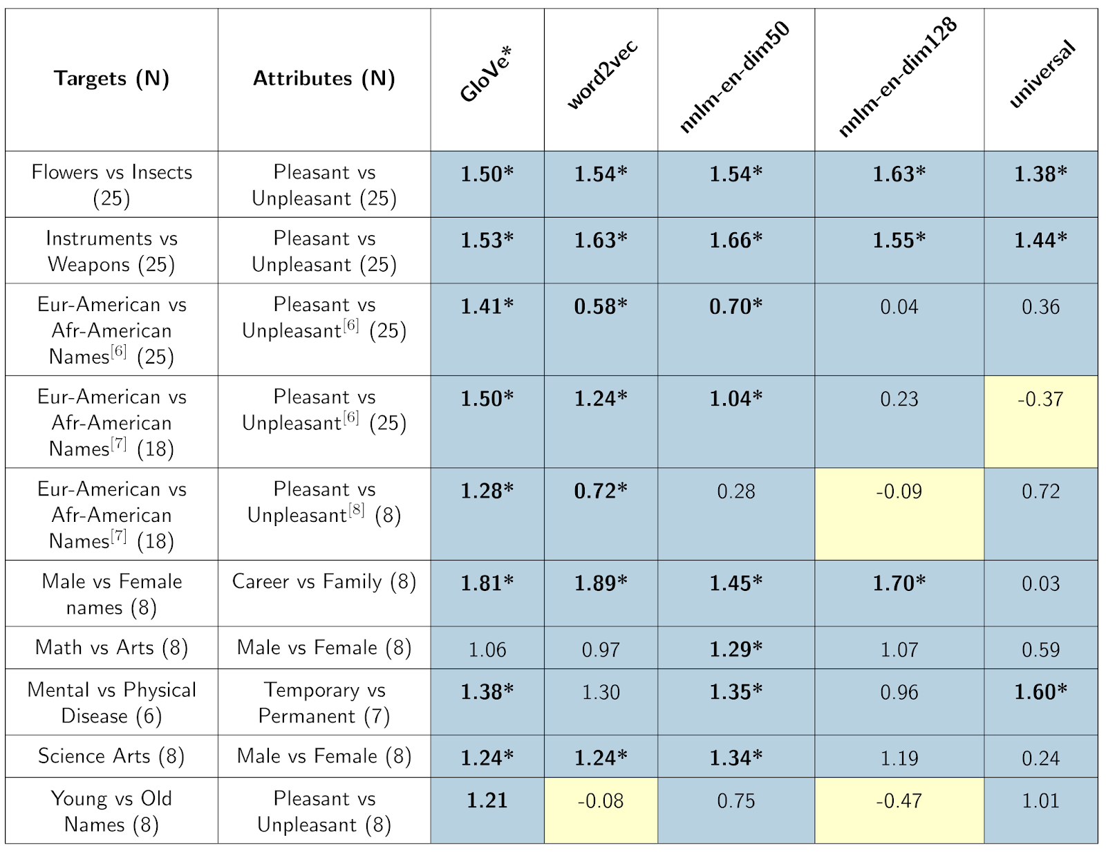
Table 1: Word Embedding Association Test (WEAT) scores for different embedding models. Cell color indicates whether the direction of the measured bias is in line with (blue) or against (yellow) the common human biases recorded by the Implicit Association Tests. *Statistically significant (p < 0.01) using Caliskan et al. (2015) permutation test. Rows 3-5 are variations whose word lists come from [6], [7], and [8]. See Caliskan et al. for all word lists. * For GloVe, we follow Caliskan et al. and drop uncommon words from the word lists. All other analyses use the full word lists.

These associations are learned from the data that was used to train these models. All of the models have learned the associations for flowers, insects, instruments, and weapons that we might expect and that may be useful in text understanding. The associations learned for the other targets vary, with some -- but not all -- models reinforcing common human biases.

For developers who use these models, it's important to be aware that these associations exist, and that these tests only evaluate a small subset of possible problematic biases. Strategies to reduce unwanted biases are a new and active area of research, and there exists no "silver bullet" that will work best for all applications.

When focusing in on associations in an embedding model, the clearest way to determine how they will affect downstream applications is by examining those applications directly. We turn now to a brief analysis of two sample applications: A Sentiment Analyzer and a Messaging App.

Case study 1: Tia's Movie Sentiment Analyzer

WEAT scores measure properties of word embeddings, but they don't tell us how those embeddings affect downstream tasks. Here we demonstrate the effect of how names are embedded in a few common embeddings on a movie review sentiment analysis task.

Tia is looking to train a sentiment classifier for movie reviews. She does not have very many samples of movie reviews, and so she leverages pretrained embeddings which map the text into a representation which can make the classification task easier.

Let's simulate Tia's scenario using an IMDB movie review dataset [9], subsampled to 1,000 positive and 1,000 negative reviews. We'll use a pre-trained word embedding to map the text of the IMDB reviews to low-dimensional vectors and use these vectors as features in a linear classifier. We'll consider a few different word embedding models and training a linear sentiment classifier with each.

We'll evaluate the quality of the sentiment classifier using the area under the ROC curve (AUC) metric on a held-out test set.

Here are AUC scores for movie sentiment classification using each of the embeddings to extract features:

Figure 3: Performance scores on the sentiment analysis task, measured in AUC, for each of the different embeddings.

At first, Tia's decision seems easy. She should use the embedding that result in the classifier with the highest score, right?

However, let's think about some other aspects that could affect this decision. The word embeddings were trained on large datasets that Tia may not have access to. She would like to assess whether biases inherent in those datasets may affect the behavior of her classifier.

Looking at the WEAT scores for various embeddings, Tia notices that some embeddings consider certain names more "pleasant" than others. That doesn't sound like a good property of a movie sentiment analyzer. It doesn't seem right to Tia that names should affect the predicted sentiment of a movie review. She decides to check whether this "pleasantness bias" affects her classification task.

She starts by constructing some test examples to determine whether a noticeable bias can be detected.

In this case, she takes the 100 shortest reviews from her test set and appends the words "reviewed by _______", where the blank is filled in with a name. Using the lists of "African American" and "European American" names from Caliskan et al. and common male and female names from the United States Social Security Administration, she looks at the difference in average sentiment scores.

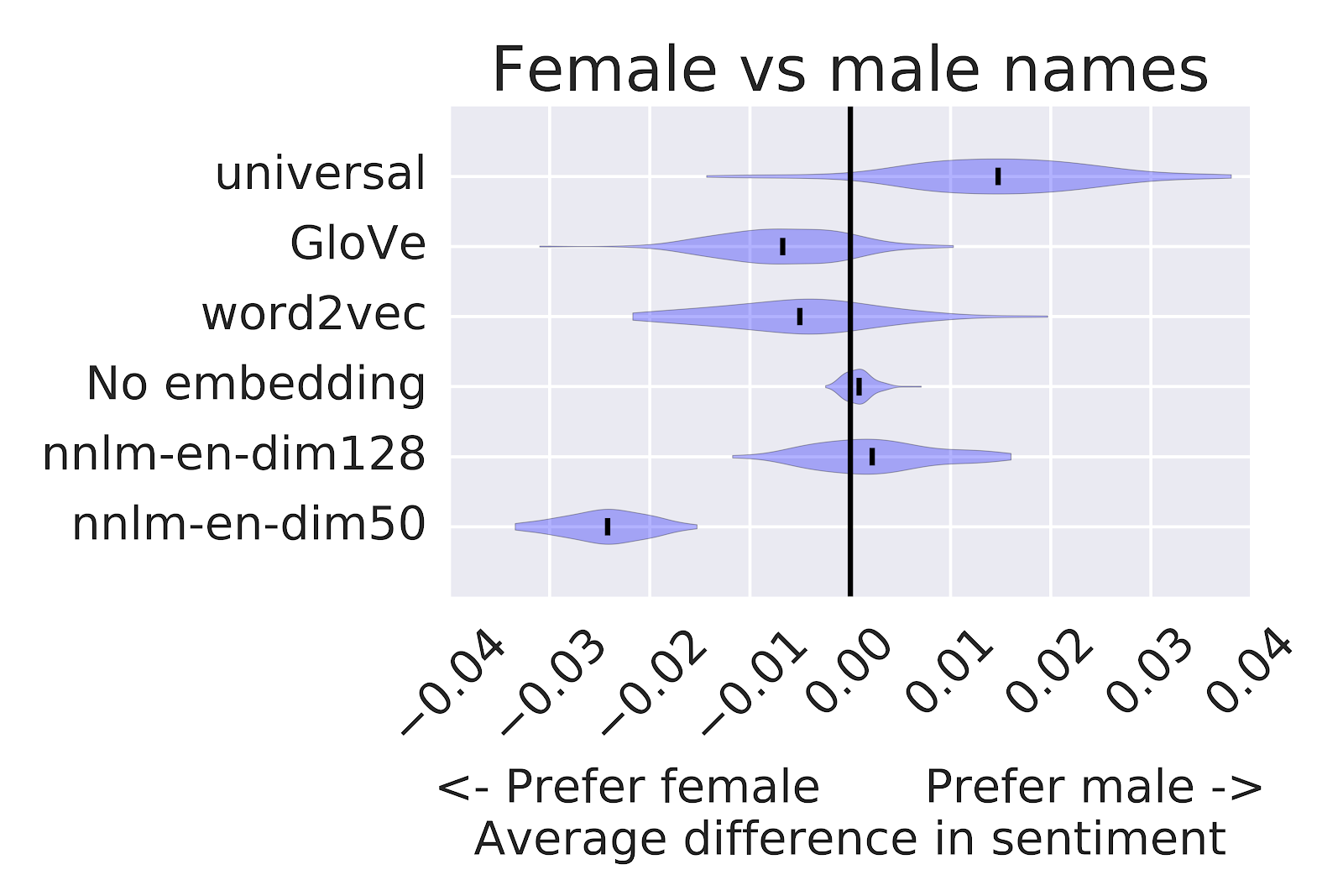
Figure 4: Difference in average sentiment scores on the modified test sets where "reviewed by ______" had been added to the end of each review. The violin plots show the distribution over differences when models are trained on small samples of the original IMDB training data.

The violin-plots above show the distribution in differences of average sentiment scores that Tia might see, simulated by taking subsamples of 1,000 positive and 1,000 negative reviews from the original IMDB training set. We show results for five word embeddings, as well as a model (No embedding) that doesn't use a word embedding.

Checking the difference in sentiment with no embedding is a good check that confirms that the sentiment associated with the names is not coming from the small IMDB supervised dataset, but rather is introduced by the pretrained embeddings. We can also see that different embeddings lead to different system outcomes, demonstrating that the choice of embedding is a key factor in the associations that Tia's sentiment classifier will make.

Tia needs to think very carefully about how this classifier will be used. Maybe her goal is just to select a few good movies for herself to watch next. In this case, it may not be a big deal. The movies that appear at the top of the list are likely to be very well-liked movies. But what if she hires and pays actors and actresses according to their average movie review ratings, as assessed by her model? That sounds much more problematic.

Tia may not be limited to the choices presented here. There are other approaches that she may consider, like mapping all names to a single word type, retraining the embeddings using data designed to mitigate sensitivity to names in her dataset, or using multiple embeddings and handling cases where the models disagree.

There is no one "right" answer here. Many of these decisions are highly context dependent and depend on Tia's intended use. There is a lot for Tia to think about as she chooses between feature extraction methods for training text classification models.

Case study 2: Tamera's Messaging App

Tamera is building a messaging app, and she wants to use text embedding models to give users suggested replies when they receive a message. She's already built a system to generate a set of candidate replies for a given message, and she wants to use a text embedding model to score these candidates. Specifically, she'll run the input message through the model to get the message embedding vector, do the same for each of the candidate responses, and then score each candidate with the cosine similarity between its embedding vector and the message embedding vector.

While there are many ways that a model's bias may play a role in these suggested replies, she decides to focus on one narrow aspect in particular: the association between occupations and binary gender. An example of bias in this context is if the incoming message is "Did the engineer finish the project?" and the model scores the response "Yes he did" higher than "Yes she did." These associations are learned from the data used to train the embeddings, and while they reflect the degree to which each gendered response is likely to be the actual response in the training data (and the degree to which there's a gender imbalance in these occupations in the real world), it can be a negative experience for users when the system simply assumes that the engineer is male.

To measure this form of bias, she creates a templated list of prompts and responses. The templates include questions such as, "Is/was your cousin a(n) ?" and "Is/was the here today?", with answer templates of "Yes, s/he is/was." For a given occupation and question (e.g., "Will the plumber be there today?"), the model's bias score is the difference between the model's score for the female-gendered response ("Yes, she will") and that of the male-gendered response ("Yes, he will"):

For a given occupation overall, the model's bias score is the sum of the bias scores for all question/answer templates with that occupation.

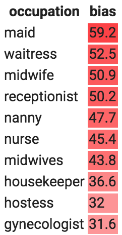
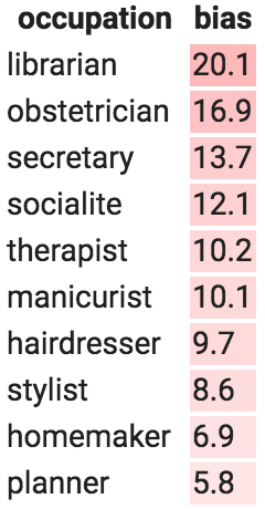
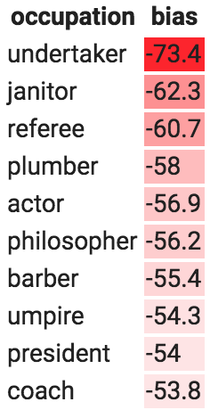
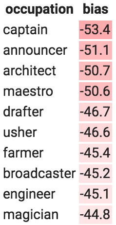
Tamera runs 200 occupations through this analysis using the Universal Sentence Encoder embedding model. Table 2 shows the occupations with the highest female-biased scores (left) and the highest male-biased scores (right):

Highest female biasHighest male bias

Table 2: Occupations with the highest female-biased scores (left) and the highest male-biased scores (right).

Tamera isn't bothered by the fact that "waitress" questions are more likely to induce a response that contains "she," but many of the other response biases give her pause. As with Tia, Tamera has several choices she can make. She could simply accept these biases as is and do nothing, though at least now she won't be caught off-guard if users complain. She could make changes in the user interface, for example by having it present two gendered responses instead of just one, though she might not want to do that if the input message has a gendered pronoun (e.g., "Will she be there today?"). She could try retraining the embedding model using a bias mitigation technique (e.g., as in Bolukbasi et al.) and examining how this affects downstream performance, or she might mitigate bias in the classifier directly when training her classifier (e.g., as in Dixon et al. [1], Beutel et al. [10], or Zhang et al. [11]). No matter what she decides to do, it's important that Tamera has done this type of analysis so that she's aware of what her product does and can make informed decisions.

Conclusions

To better understand the potential issues that an ML model might create, both model creators and practitioners who use these models should examine the undesirable biases that models may contain. We've shown some tools for uncovering particular forms of stereotype bias in these models, but this certainly doesn't constitute all forms of bias. Even the WEAT analyses discussed here are quite narrow in scope, and so should not be interpreted as capturing the full story on implicit associations in embedding models. For example, a model trained explicitly to eliminate negative associations for 50 names in one of the WEAT categories would likely not mitigate negative associations for other names or categories, and the resulting low WEAT score could give a false sense that negative associations as a whole have been well addressed. These evaluations are better used to inform us about the way existing models behave and to serve as one starting point in understanding how unwanted biases can affect the technology that we make and use. We're continuing to work on this problem because we believe it's important and we invite you to join this conversation as well.

Acknowledgments

We would like to thank Lucy Vasserman, Eric Breck, Erica Greene, and the TensorFlow Hub and Semantic Experiences teams for collaborating on this work.

References

[1] Dixon, L., Li, J., Sorensen, J., Thain, M. and Vasserman, L., 2018. Measuring and Mitigating Unintended Bias in Text Classification. AIES.

[2] Buolamwini, J. and Gebru, T., 2018. Gender Shades: Intersectional Accuracy Disparities in Commercial Gender Classification. FAT/ML.

[3] Tatman, R. and Kasten, C. 2017. Effects of Talker Dialect, Gender & Race on Accuracy of Bing Speech and YouTube Automatic Captions. INTERSPEECH.

[4] Bolukbasi, T., Chang, K., Zou, J., Saligrama, V. and Kalai, A. 2016. Man is to Computer Programmer as Woman is to Homemaker? Debiasing Word Embeddings. NIPS.

[5] Caliskan, A., Bryson, J. J. and Narayanan, A. 2017. Semantics derived automatically from language corpora contain human-like biases. Science.

[6] Greenwald, A. G., McGhee, D. E., and Schwartz, J. L. 1998. Measuring individual differences in implicit cognition: the implicit association test. Journal of personality and social psychology.

[7] Bertrand, M. and Mullainathan, S. 2004. Are emily and greg more employable than lakisha and jamal? a field experiment on labor market discrimination. The American Economic Review.

[8] Nosek, B. A., Banaji, M., and Greenwald, A. G. 2002. Harvesting implicit group attitudes and beliefs from a demonstration web site. Group Dynamics: Theory, Research, and Practice.

[9] Andrew L. Maas, Raymond E. Daly, Peter T. Pham, Dan Huang, Andrew Y. Ng, and Christopher Potts. 2011. Learning Word Vectors for Sentiment Analysis. ACL.

[10] Beutel, A., Chen, J., Zhao, Z., & Chi, E. H. 2017 Data Decisions and Theoretical Implications when Adversarially Learning Fair Representations. FAT/ML.

[11] Zhang, B., Lemoine, B., and Mitchell, M. 2018. Mitigating Unwanted Biases with Adversarial Learning. AIES.

How to make AI that’s good for people

For a field that was not well known outside of academia a decade ago, artificial intelligence has grown dizzyingly fast. Tech companies from Silicon Valley to Beijing are betting everything on it, venture capitalists are pouring billions into research and development, and start-ups are being created on what seems like a daily basis. If our era is the next Industrial Revolution, as many claim, AI is surely one of its driving forces.

It is an especially exciting time for a researcher like me. When I was a graduate student in computer science in the early 2000s, computers were barely able to detect sharp edges in photographs, let alone recognize something as loosely defined as a human face. But thanks to the growth of big data, advances in algorithms like neural networks and an abundance of powerful computer hardware, something momentous has occurred: AI has gone from an academic niche to the leading differentiator in a wide range of industries, including manufacturing, health care, transportation and retail.

I worry, however, that enthusiasm for AI is preventing us from reckoning with its looming effects on society. Despite its name, there is nothing “artificial” about this technology—it is made by humans, intended to behave like humans and affects humans. So if we want it to play a positive role in tomorrow’s world, it must be guided by human concerns.

I call this approach “human-centered AI.” It consists of three goals that can help responsibly guide the development of intelligent machines.

First, AI needs to reflect more of the depth that characterizes our own intelligence. Consider the richness of human visual perception. It’s complex and deeply contextual, and naturally balances our awareness of the obvious with a sensitivity to nuance. By comparison, machine perception remains strikingly narrow.

Sometimes this difference is trivial. For instance, in my lab, an image-captioning algorithm once fairly summarized a photo as “a man riding a horse” but failed to note the fact that both were bronze sculptures. Other times, the difference is more profound, as when the same algorithm described an image of zebras grazing on a savanna beneath a rainbow. While the summary was technically correct, it was entirely devoid of aesthetic awareness, failing to detect any of the vibrancy or depth a human would naturally appreciate.

That may seem like a subjective or inconsequential critique, but it points to a major aspect of human perception beyond the grasp of our algorithms. How can we expect machines to anticipate our needs—much less contribute to our well-being—without insight into these “fuzzier” dimensions of our experience?

Making AI more sensitive to the full scope of human thought is no simple task. The solutions are likely to require insights derived from fields beyond computer science, which means programmers will have to learn to collaborate more often with experts in other domains.

Such collaboration would represent a return to the roots of our field, not a departure from it. Younger AI enthusiasts may be surprised to learn that the principles of today’s deep-learning algorithms stretch back more than 60 years to the neuroscientific researchers David Hubel and Torsten Wiesel, who discovered how the hierarchy of neurons in a cat’s visual cortex responds to stimuli.

Likewise, ImageNet, a data set of millions of training photographs that helped to advance computer vision, is based on a project called WordNet, created in 1995 by the cognitive scientist and linguist George Miller. WordNet was intended to organize the semantic concepts of English.

Reconnecting AI with fields like cognitive science, psychology and even sociology will give us a far richer foundation on which to base the development of machine intelligence. And we can expect the resulting technology to collaborate and communicate more naturally, which will help us approach the second goal of human-centered AI: enhancing us, not replacing us.

Imagine the role that AI might play during surgery. The goal need not be to automate the process entirely. Instead, a combination of smart software and specialized hardware could help surgeons focus on their strengths—traits like dexterity and adaptability—while keeping tabs on more mundane tasks and protecting against human error, fatigue and distraction.

Or consider senior care. Robots may never be the ideal custodians of the elderly, but intelligent sensors are already showing promise in helping human caretakers focus more on their relationships with those they provide care for by automatically monitoring drug dosages and going through safety checklists.

These are examples of a trend toward automating those elements of jobs that are repetitive, error-prone and even dangerous. What’s left are the creative, intellectual and emotional roles for which humans are still best suited.

No amount of ingenuity, however, will fully eliminate the threat of job displacement. Addressing this concern is the third goal of human-centered AI: ensuring that the development of this technology is guided, at each step, by concern for its effect on humans.

Today’s anxieties over labor are just the start. Additional pitfalls include bias against underrepresented communities in machine learning, the tension between AI’s appetite for data and the privacy rights of individuals and the geopolitical implications of a global intelligence race.

Adequately facing these challenges will require commitments from many of our largest institutions. Universities are uniquely positioned to foster connections between computer science and traditionally unrelated departments like the social sciences and even humanities, through interdisciplinary projects, courses and seminars. Governments can make a greater effort to encourage computer science education, especially among young girls, racial minorities and other groups whose perspectives have been underrepresented in AI. And corporations should combine their aggressive investment in intelligent algorithms with ethical AI policies that temper ambition with responsibility.

No technology is more reflective of its creators than AI. It has been said that there are no “machine” values at all, in fact; machine values are human values. A human-centered approach to AI means these machines don’t have to be our competitors, but partners in securing our well-being. However autonomous our technology becomes, its impact on the world—for better or worse—will always be our responsibility.

This article was originally published in the New York Times.

Noodle on this: Machine learning that can identify ramen by shop

There are casual ramen fans and then there are ramen lovers. There are people who are all tonkatsu all the time, and others who swear by tsukemen. And then there’s machine learning, which—based on a recent case study out of Japan—might be the biggest ramen aficionado of them all.


Recently, data scientist Kenji Doi used machine learning models and AutoML Vision to classify bowls of ramen and identify the exact shop each bowl is made at, out of 41 ramen shops, with 95 percent accuracy. Sounds crazy (also delicious), especially when you see what these bowls look like:
Ramen bowls made at three different Ramen Jiro shops.
Ramen bowls made at three different Ramen Jiro shops

With 41 locations around Tokyo, Ramen Jiro is one of the most popular restaurant franchises in Japan, because of its generous portions of toppings, noodles and soup served at low prices. They serve the same basic menu at each shop, and as you can see above, it's almost impossible for a human (especially if you're new to Ramen Jiro) to tell what shop each bowl is made at.


But Kenji thought deep learning could discern the minute details that make one shop’s bowl of ramen different from the next. He had already built a machine learning model to classify ramen, but wanted to see if AutoML Vision could do it more efficiently.


AutoML Vision creates customized ML models automatically—to identify animals in the wild, or recognize types of products to improve an online store, or in this case classify ramen. You don’t have to be a data scientist to know how to use it—all you need to do is upload well-labeled images and then click a button. In Kenji’s case, he compiled a set of 48,000 photos of bowls of soup from Ramen Jiro locations, along with labels for each shop, and uploaded them to AutoML Vision. The model took about 24 hours to train, all automatically (although a less accurate, “basic” mode had a model ready in just 18 minutes). The results were impressive: Kenji’s model got 94.5 percentaccuracy on predicting the shop just from the photos.

Confusion matrix of Ramen Jiro shop classifier by AutoML Vision

Confusion matrix of Ramen Jiro shop classifier by AutoML Vision (Advanced mode). Row = actual shop, column = predicted shop. You can see AutoML Vision incorrectly identified the restaurant location in only a couple of instances for each test case.

AutoML Vision is designed for people without ML expertise, but it also speeds things up dramatically for experts. Building a model for ramen classification from scratch would be a time-consuming process requiring multiple steps—labeling, hyperparameter tuning, multiple attempts with different neural net architectures, and even failed training runs—and experience as a data scientist. As Kenji puts it, “With AutoML Vision, a data scientist wouldn’t need to spend a long time training and tuning a model to achieve the best results. This means businesses could scale their AI work even with a limited number of data scientists." We wrote about another recent example of AutoML Vision at work in this Big Data blog post, which also has more technical details on Kenji’s model.


As for how AutoML detects the differences in ramen, it’s certainly not from the taste. Kenji’s first hypothesis was that the model was looking at the color or shape of the bowl or table—but that seems unlikely, since the model was highly accurate even when each shop used the same bowl and table design. Kenji’s new theory is that the model is accurate enough to distinguish very subtle differences between cuts of the meat, or the way toppings are served. He plans on continuing to experiment with AutoML to see if his theories are true. Sounds like a project that might involve more than a few bowls of ramen. Slurp on.

Source: Google Cloud


Using Machine Learning to Discover Neural Network Optimizers


Deep learning models have been deployed in numerous Google products, such as Search, Translate and Photos. The choice of optimization method plays a major role when training deep learning models. For example, stochastic gradient descent works well in many situations, but more advanced optimizers can be faster, especially for training very deep networks. Coming up with new optimizers for neural networks, however, is challenging due to to the non-convex nature of the optimization problem. On the Google Brain team, we wanted to see if it could be possible to automate the discovery of new optimizers, in a way that is similar to how AutoML has been used to discover new competitive neural network architectures.

In “Neural Optimizer Search with Reinforcement Learning”, we present a method to discover optimization methods with a focus on deep learning architectures. Using this method we found two new optimizers, PowerSign and AddSign, that are competitive on a variety of different tasks and architectures, including ImageNet classification and Google’s neural machine translation system. To help others benefit from this work we have made the optimizers available in Tensorflow.

Neural Optimizer Search makes use of a recurrent neural network controller which is given access to a list of simple primitives that are typically relevant for optimization. These primitives include, for example, the gradient or the running average of the gradient and lead to search spaces with over 1010 possible combinations. The controller then generates the computation graph for a candidate optimizer or update rule in that search space.

In our paper, proposed candidate update rules (U) are used to train a child convolutional neural network on CIFAR10 for a few epochs and the final validation accuracy (R) is fed as a reward to the controller. The controller is trained with reinforcement learning to maximize the validation accuracies of the sampled update rules. This process is illustrated below.
An overview of Neural Optimizer Search using an iterative process to discover new optimizers.
Interestingly, the optimizers we have found are interpretable. For example, in the PowerSign optimizer we are releasing, each update compares the sign of the gradient and its running average, adjusting the step size according to whether those two values agree. The intuition behind this is that if these values agree, one is more confident in the direction of the update, and thus the step size can be larger. We also discovered a simple learning rate decay scheme, linear cosine decay, which we found can lead to faster convergence.
Graph comparing learning rate decay functions for linear cosine decay, stepwise decay and cosine decay.
Neural Optimizer Search found several optimizers that outperform commonly used optimizers on the small ConvNet model. Among the ones that transfer well to other tasks, we found that PowerSign and AddSign improve top-1 and top-5 accuracy of a state-of-the-art ImageNet mobile-sized model by up to 0.4%. They also work well on Google’s Neural Machine Translation system, giving an improvement of up to 0.7 using bilingual evaluation metrics (BLEU) on an English to German translation task.

We are excited that Neural Optimizer Search can not only improve the performance of machine learning models but also potentially lead to new, interpretable equations and discoveries. It is our hope that open sourcing these optimizers in Tensorflow will be useful to machine learning practitioners.

Source: Google AI Blog


Using Machine Learning to Discover Neural Network Optimizers


Deep learning models have been deployed in numerous Google products, such as Search, Translate and Photos. The choice of optimization method plays a major role when training deep learning models. For example, stochastic gradient descent works well in many situations, but more advanced optimizers can be faster, especially for training very deep networks. Coming up with new optimizers for neural networks, however, is challenging due to to the non-convex nature of the optimization problem. On the Google Brain team, we wanted to see if it could be possible to automate the discovery of new optimizers, in a way that is similar to how AutoML has been used to discover new competitive neural network architectures.

In “Neural Optimizer Search with Reinforcement Learning”, we present a method to discover optimization methods with a focus on deep learning architectures. Using this method we found two new optimizers, PowerSign and AddSign, that are competitive on a variety of different tasks and architectures, including ImageNet classification and Google’s neural machine translation system. To help others benefit from this work we have made the optimizers available in Tensorflow.

Neural Optimizer Search makes use of a recurrent neural network controller which is given access to a list of simple primitives that are typically relevant for optimization. These primitives include, for example, the gradient or the running average of the gradient and lead to search spaces with over 1010 possible combinations. The controller then generates the computation graph for a candidate optimizer or update rule in that search space.

In our paper, proposed candidate update rules (U) are used to train a child convolutional neural network on CIFAR10 for a few epochs and the final validation accuracy (R) is fed as a reward to the controller. The controller is trained with reinforcement learning to maximize the validation accuracies of the sampled update rules. This process is illustrated below.
An overview of Neural Optimizer Search using an iterative process to discover new optimizers.
Interestingly, the optimizers we have found are interpretable. For example, in the PowerSign optimizer we are releasing, each update compares the sign of the gradient and its running average, adjusting the step size according to whether those two values agree. The intuition behind this is that if these values agree, one is more confident in the direction of the update, and thus the step size can be larger. We also discovered a simple learning rate decay scheme, linear cosine decay, which we found can lead to faster convergence.
Graph comparing learning rate decay functions for linear cosine decay, stepwise decay and cosine decay.
Neural Optimizer Search found several optimizers that outperform commonly used optimizers on the small ConvNet model. Among the ones that transfer well to other tasks, we found that PowerSign and AddSign improve top-1 and top-5 accuracy of a state-of-the-art ImageNet mobile-sized model by up to 0.4%. They also work well on Google’s Neural Machine Translation system, giving an improvement of up to 0.7 using bilingual evaluation metrics (BLEU) on an English to German translation task.

We are excited that Neural Optimizer Search can not only improve the performance of machine learning models but also potentially lead to new, interpretable equations and discoveries. It is our hope that open sourcing these optimizers in Tensorflow will be useful to machine learning practitioners.

The fight against illegal deforestation with TensorFlow

Editor’s Note: Rainforest Connection is using technology to protect the rainforest. Founder and CEO Topher White shares how TensorFlow, Google’s open-source machine learning framework, aids in their efforts.

For me, growing up in the 80s and 90s, the phrase “Save the Rainforest” was a directive that barely progressed over the years. The appeal was clear, but the threat was abstract and distant. And the solution (if there was one) seemed difficult to grasp. Since then, other worries—even harder to grasp in their immediacy and scope—have come to dominate our conversations: climate change, as an example.

So many of us believe that technology has a crucial role to play in fighting climate change, but few are as aware that “Saving the Rainforest” and fighting climate change are nearly one and the same. By the numbers, destruction of forests accounts for nearly one-fifth of all greenhouse gas emissions every year. And in the tropical rainforest deforestation accelerated on the heels of rampant logging—up to 90 percent of which is done illegally and under the radar.

Stopping illegal logging and protecting the world’s rainforests may be the fastest, cheapest way for humanity to slow climate change. And who’s best suited to protect the rainforest? The locals and the indigenous tribes that have lived there for generations.

Rainforest Connection is a group of engineers and developers focused on building technology to help locals—like the Tembé tribe from central Amazon—protect their land, and in the process, protect the rest of us from the effects of climate change. Chief Naldo Tembé reached out to me a couple years ago seeking to collaborate on ways technology could help stop illegal loggers from destroying their land. Together, we embarked on an ambitious plan to address this issue using recycled cell phones and machine learning.

Our team has built the world’s first scalable, real-time detection and alert system for logging and environmental conservation in the rainforest. Building hardware that will survive in the rainforest is challenging, but we’re using what’s already there: the trees. We’ve hidden modified smartphones powered with solar panels—called “Guardian” devices—in trees in threatened areas, and continuously monitor the sounds of the forest, sending all audio up to our cloud-based servers over the standard, local cell-­phone network.

Once the audio is in the cloud, we use TensorFlow, Google’s machine learning framework, to analyze all the auditory data in real-time and listen for chainsaws, logging trucks and other sounds of illegal activity that can help us pinpoint problems in the forest. Audio pours in constantly from every phone, 24 hours a day, every day, and the stakes of missed detections are high.

That’s why we’ve come to use TensorFlow, due to its ability to analyze every layer of our data heavy detection process. The versatility of the machine learning framework empowers us to use a wide range of AI techniques with Deep Learning on one unified platform. This allows us to tweak our audio inputs and improve detection quality. Without the help of machine learning, this process is impossible. When fighting deforestation, every improvement can mean one more saved tree.

The next step is to involve those who will inherit the planet from us: kids. Today, we’re launching the “Planet Guardians” program with hundreds of students from Los Angeles STEM science programs. These students will speak with the local Tembé Tribe through Google Hangouts, and build their own Guardian devices to be sent to the Amazon. We expect that the Guardian devices built by these LA students will protect nearly 100,000 acres through the year 2020.

With technology, and the possibilities that TensorFlow opens up for us, Rainforest Connection will continue to do our part in the fight against climate change. And programs like “Planet Guardians” will ensure that the next generation is a part of this fight, too.

Making music using new sounds generated with machine learning

Technology has always played a role in inspiring musicians in new and creative ways. The guitar amp gave rock musicians a new palette of sounds to play with in the form of feedback and distortion. And the sounds generated by synths helped shape the sound of electronic music. But what about new technologies like machine learning models and algorithms? How might they play a role in creating new tools and possibilities for a musician’s creative process? Magenta, a research project within Google, is currently exploring answers to these questions.

Building upon past research in the field of machine learning and music, last year Magenta released NSynth (Neural Synthesizer). It’s a machine learning algorithm that uses deep neural networks to learn the characteristics of sounds, and then create a completely new sound based on these characteristics. Rather than combining or blending the sounds, NSynth synthesizes an entirely new sound using the acoustic qualities of the original sounds—so you could get a sound that’s part flute and part sitar all at once.

Since then, Magenta has continued to experiment with different musical interfaces and tools to make the algorithm more easily accessible and playable. As part of this exploration, Google Creative Lab and Magenta collaborated to create NSynth Super. It’s an open source experimental instrument which gives musicians the ability to explore new sounds generated with the NSynth algorithm.

Making music using new sounds generated with machine learning

To create our prototype, we recorded 16 original source sounds across a range of 15 pitches and fed them into the NSynth algorithm. The outputs, over 100,000 new sounds, were then loaded into NSynth Super to precompute the new sounds. Using the dials, musicians can select the source sounds they would like to explore between, and drag their finger across the touchscreen to navigate the new, unique sounds which combine their acoustic qualities. NSynth Super can be played via any MIDI source, like a DAW, sequencer or keyboard.

03. NSynth-Super-Bathing_2880x1800.jpg

Part of the goal of Magenta is to close the gap between artistic creativity and machine learning. It’s why we work with a community of artists, coders and machine learning researchers to learn more about how machine learning tools might empower creators. It’s also why we create everything, including NSynth Super, with open source libraries, including TensorFlow and openFrameworks. If you’re maker, musician, or both, all of the source code, schematics, and design templates are available for download on GitHub.

04. Open-NSynth-Super-Parts-2880x1800.jpg

New sounds are powerful. They can inspire musicians in creative and unexpected ways, and sometimes they might go on to define an entirely new musical style or genre. It’s impossible to predict where the new sounds generated by machine learning tools might take a musician, but we're hoping they lead to even more musical experimentation and creativity.


Learn more about NSynth Super at g.co/nsynthsuper.

Understanding the inner workings of neural networks

Neural networks are a powerful approach to machine learning, allowing computers to understand images, recognize speech, translate sentences, play Go, and much more. As much as we’re using neural networks in our technology at Google, there’s more to learn about how these systems accomplish these feats. For example, neural networks can learn how to recognize images far more accurately than any program we directly write, but we don’t really know how exactly they decide whether a dog in a picture is a Retriever, a Beagle, or a German Shepherd.

We’ve been working for several years to better grasp how neural networks operate. Last week we shared new research on how these techniques come together to give us a deeper understanding of why networks make the decisions they do—but first, let’s take a step back to explain how we got here.

Neural networks consist of a series of “layers,” and their understanding of an image evolves over the course of multiple layers. In 2015, we started a project called DeepDream to get a sense of what neural networks “see” at the different layers. Itled to a much larger research project that would not only develop beautiful art, but also shed light on the inner workings of neural networks.

pasted image 0 (11).png
Outside Google, DeepDream grew into a small art movement producing all sorts of amazing things.

Last year, we shared new work on this subject, showing how techniques building on DeepDream—and lots of excellent research from our colleagues around the world—can help us explore how neural networks build up their understanding of images. We showed that neural networks build on previous layers to detect more sophisticated ideas and eventually reach complex conclusions. For instance, early layers detect edges and textures of images, but later layers progress to detecting parts of objects.

pasted image 0 (12).png
The neural network first detects edges, then textures, patterns, parts, and objects.

Last week we released another milestone in our research: an exploration of how different techniques for understanding neural networks fit together into a bigger picture.

This work, which we've published in the online journal Distill, explores how different techniques allow us to “stand in the middle of a neural network” and see how decisions made at an individual point influence a final output. For instance, we can see how a network detects a “floppy ear,” and then that increases the probability that the image will be labeled as a Labrador Retriever or Beagle.

In one example, we explore which neurons activate in response to different inputs—a kind of “MRI for neural networks.” The network has some floppy ear detectors that really like this dog!

SemanticDict2-ezgif-crop.gif

We can also see how different neurons in the middle of the network—like those floppy ear detectors—affect the decision to classify an image as a Labrador Retriever or tiger cat.

pasted image 0 (13).png

If you want to learn more, check out our interactive paper, published in Distill. We’ve also open sourced our neural net visualization library, Lucid, so you can make these visualizations, too.

One Shining AI Moment: when machine learning meets your bracket

The stats. The uniforms. Sheer wild guesses. Everyone has a strategy for making their picks for the NCAA’s March Madness tournament. But this year there’s a new play in the book: machine learning.


Google Cloud has teamed up with the NCAA to host a competition on Kaggle, the world's largest online community of data scientists, challenging participants to build and train machine learning models to forecast the games’ outcomes. Kaggle has hosted contests for the tournament in the past, but this year’s competition is taking things to the next round with a new data set that contains every play-by-play moment in men’s and women’s NCAA Division I basketball since 2009—more than 40 million plays.


The submission deadline for the competition is this Thursday, prior to the start of the tournament. Submissions will be scored by log loss, a common way of measuring accuracy of machine learning models. A total of $100,000 will be awarded across both the men’s and women’s competitions for the best performing applications of machine learning (which probably outdoes whatever happens in your office pool). And because the competition is based on ML models, not basketball know-how, it’s anyone’s game to win. Talk about a Cinderella story.


The massive data set being used in this competition represents just one area where Google Cloud is teaming up with the NCAA as their official public cloud provider. The NCAA is also in the process of migrating 80+ years of data across 24 sports to Google Cloud Platform (GCP), using Google tools to power analyses of teams and players. But for the data scientists and machine learning enthusiasts participating in the Kaggle competition, the fun is already underway. May the best model survive, advance and take home the championship!

Open Sourcing the Hunt for Exoplanets


Recently, we discovered two exoplanets by training a neural network to analyze data from NASA’s Kepler space telescope and accurately identify the most promising planet signals. And while this was only an initial analysis of ~700 stars, we consider this a successful proof-of-concept for using machine learning to discover exoplanets, and more generally another example of using machine learning to make meaningful gains in a variety of scientific disciplines (e.g. healthcare, quantum chemistry, and fusion research).

Today, we’re excited to release our code for processing the Kepler data, training our neural network model, and making predictions about new candidate signals. We hope this release will prove a useful starting point for developing similar models for other NASA missions, like K2 (Kepler’s second mission) and the upcoming Transiting Exoplanet Survey Satellite mission. As well as announcing the release of our code, we’d also like take this opportunity to dig a bit deeper into how our model works.

A Planet Hunting Primer

First, let’s consider how data collected by the Kepler telescope is used to detect the presence of a planet. The plot below is called a light curve, and it shows the brightness of the star (as measured by Kepler’s photometer) over time. When a planet passes in front of the star, it temporarily blocks some of the light, which causes the measured brightness to decrease and then increase again shortly thereafter, causing a “U-shaped” dip in the light curve.
A light curve from the Kepler space telescope with a “U-shaped” dip that indicates a transiting exoplanet.
However, other astronomical and instrumental phenomena can also cause the measured brightness of a star to decrease, including binary star systems, starspots, cosmic ray hits on Kepler’s photometer, and instrumental noise.
The first light curve has a “V-shaped” pattern that tells us that a very large object (i.e. another star) passed in front of the star that Kepler was observing. The second light curve contains two places where the brightness decreases, which indicates a binary system with one bright and one dim star: the larger dip is caused by the dimmer star passing in front of the brighter star, and vice versa. The third light curve is one example of the many other non-planet signals where the measured brightness of a star appears to decrease.
To search for planets in Kepler data, scientists use automated software (e.g. the Kepler data processing pipeline) to detect signals that might be caused by planets, and then manually follow up to decide whether each signal is a planet or a false positive. To avoid being overwhelmed with more signals than they can manage, the scientists apply a cutoff to the automated detections: those with signal-to-noise ratios above a fixed threshold are deemed worthy of follow-up analysis, while all detections below the threshold are discarded. Even with this cutoff, the number of detections is still formidable: to date, over 30,000 detected Kepler signals have been manually examined, and about 2,500 of those have been validated as actual planets!

Perhaps you’re wondering: does the signal-to-noise cutoff cause some real planet signals to be missed? The answer is, yes! However, if astronomers need to manually follow up on every detection, it’s not really worthwhile to lower the threshold, because as the threshold decreases the rate of false positive detections increases rapidly and actual planet detections become increasingly rare. However, there’s a tantalizing incentive: it’s possible that some potentially habitable planets like Earth, which are relatively small and orbit around relatively dim stars, might be hiding just below the traditional detection threshold — there might be hidden gems still undiscovered in the Kepler data!

A Machine Learning Approach

The Google Brain team applies machine learning to a diverse variety of data, from human genomes to sketches to formal mathematical logic. Considering the massive amount of data collected by the Kepler telescope, we wondered what we might find if we used machine learning to analyze some of the previously unexplored Kepler data. To find out, we teamed up with Andrew Vanderburg at UT Austin and developed a neural network to help search the low signal-to-noise detections for planets.
We trained a convolutional neural network (CNN) to predict the probability that a given Kepler signal is caused by a planet. We chose a CNN because they have been very successful in other problems with spatial and/or temporal structure, like audio generation and image classification.
Luckily, we had 30,000 Kepler signals that had already been manually examined and classified by humans. We used a subset of around 15,000 of these signals, of which around 3,500 were verified planets or strong planet candidates, to train our neural network to distinguish planets from false positives. The inputs to our network are two separate views of the same light curve: a wide view that allows the model to examine signals elsewhere on the light curve (e.g., a secondary signal caused by a binary star), and a zoomed-in view that enables the model to closely examine the shape of the detected signal (e.g., to distinguish “U-shaped” signals from “V-shaped” signals).

Once we had trained our model, we investigated the features it learned about light curves to see if they matched with our expectations. One technique we used (originally suggested in this paper) was to systematically occlude small regions of the input light curves to see whether the model’s output changed. Regions that are particularly important to the model’s decision will change the output prediction if they are occluded, but occluding unimportant regions will not have a significant effect. Below is a light curve from a binary star that our model correctly predicts is not a planet. The points highlighted in green are the points that most change the model’s output prediction when occluded, and they correspond exactly to the secondary “dip” indicative of a binary system. When those points are occluded, the model’s output prediction changes from ~0% probability of being a planet to ~40% probability of being a planet. So, those points are part of the reason the model rejects this light curve, but the model uses other evidence as well - for example, zooming in on the centred primary dip shows that it's actually “V-shaped”, which is also indicative of a binary system.

Searching for New Planets

Once we were confident with our model’s predictions, we tested its effectiveness by searching for new planets in a small set 670 stars. We chose these stars because they were already known to have multiple orbiting planets, and we believed that some of these stars might host additional planets that had not yet been detected. Importantly, we allowed our search to include signals that were below the signal-to-noise threshold that astronomers had previously considered. As expected, our neural network rejected most of these signals as spurious detections, but a handful of promising candidates rose to the top, including our two newly discovered planets: Kepler-90 i and Kepler-80 g.

Find your own Planet(s)!

Let’s take a look at how the code released today can help (re-)discover the planet Kepler-90 i. The first step is to train a model by following the instructions on the code’s home page. It takes a while to download and process the data from the Kepler telescope, but once that’s done, it’s relatively fast to train a model and make predictions about new signals. One way to find new signals to show the model is to use an algorithm called Box Least Squares (BLS), which searches for periodic “box shaped” dips in brightness (see below). The BLS algorithm will detect “U-shaped” planet signals, “V-shaped” binary star signals and many other types of false positive signals to show the model. There are various freely available software implementations of the BLS algorithm, including VARTOOLS and LcTools. Alternatively, you can even look for candidate planet transits by eye, like the Planet Hunters.
A low signal-to-noise detection in the light curve of the Kepler 90 star detected by the BLS algorithm. The detection has period 14.44912 days, duration 2.70408 hours (0.11267 days) beginning 2.2 days after 12:00 on 1/1/2009 (the year the Kepler telescope launched).
To run this detected signal though our trained model, we simply execute the following command:
python predict.py  --kepler_id=11442793 --period=14.44912 --t0=2.2
--duration=0.11267 --kepler_data_dir=$HOME/astronet/kepler
--output_image_file=$HOME/astronet/kepler-90i.png
--model_dir=$HOME/astronet/model
The output of the command is prediction = 0.94, which means the model is 94% certain that this signal is a real planet. Of course, this is only a small step in the overall process of discovering and validating an exoplanet: the model’s prediction is not proof one way or the other. The process of validating this signal as a real exoplanet requires significant follow-up work by an expert astronomer — see Sections 6.3 and 6.4 of our paper for the full details. In this particular case, our follow-up analysis validated this signal as a bona fide exoplanet, and it’s now called Kepler-90 i!
Our work here is far from done. We’ve only searched 670 stars out of 200,000 observed by Kepler — who knows what we might find when we turn our technique to the entire dataset. Before we do that, though, we have a few improvements we want to make to our model. As we discussed in our paper, our model is not yet as good at rejecting binary stars and instrumental false positives as some more mature computer heuristics. We’re hard at work improving our model, and now that it’s open sourced, we hope others will do the same!


By Chris Shallue, Senior Software Engineer, Google Brain Team

If you’d like to learn more, Chris is featured on the latest episode of This Week In Machine Learning discussing his work.