Tag Archives: deep learning

Constructing Transformers For Longer Sequences with Sparse Attention Methods

Natural language processing (NLP) models based on Transformers, such as BERT, RoBERTa, T5, or GPT3, are successful for a wide variety of tasks and a mainstay of modern NLP research. The versatility and robustness of Transformers are the primary drivers behind their wide-scale adoption, leading them to be easily adapted for a diverse range of sequence-based tasks — as a seq2seq model for translation, summarization, generation, and others, or as a standalone encoder for sentiment analysis, POS tagging, machine reading comprehension, etc. The key innovation in Transformers is the introduction of a self-attention mechanism, which computes similarity scores for all pairs of positions in an input sequence, and can be evaluated in parallel for each token of the input sequence, avoiding the sequential dependency of recurrent neural networks, and enabling Transformers to vastly outperform previous sequence models like LSTM.

A limitation of existing Transformer models and their derivatives, however, is that the full self-attention mechanism has computational and memory requirements that are quadratic with the input sequence length. With commonly available current hardware and model sizes, this typically limits the input sequence to roughly 512 tokens, and prevents Transformers from being directly applicable to tasks that require larger context, like question answering, document summarization or genome fragment classification. Two natural questions arise: 1) Can we achieve the empirical benefits of quadratic full Transformers using sparse models with computational and memory requirements that scale linearly with the input sequence length? 2) Is it possible to show theoretically that these linear Transformers preserve the expressivity and flexibility of the quadratic full Transformers?

We address both of these questions in a recent pair of papers. In “ETC: Encoding Long and Structured Inputs in Transformers”, presented at EMNLP 2020, we present the Extended Transformer Construction (ETC), which is a novel method for sparse attention, in which one uses structural information to limit the number of computed pairs of similarity scores. This reduces the quadratic dependency on input length to linear and yields strong empirical results in the NLP domain. Then, in “Big Bird: Transformers for Longer Sequences”, presented at NeurIPS 2020, we introduce another sparse attention method, called BigBird that extends ETC to more generic scenarios where prerequisite domain knowledge about structure present in the source data may be unavailable. Moreover, we also show that theoretically our proposed sparse attention mechanism preserves the expressivity and flexibility of the quadratic full Transformers. Our proposed methods achieve a new state of the art on challenging long-sequence tasks, including question answering, document summarization and genome fragment classification.

Attention as a Graph
The attention module used in Transformer models computes similarity scores for all pairs of positions in an input sequence. It is useful to think of the attention mechanism as a directed graph, with tokens represented by nodes and the similarity score computed between a pair of tokens represented by an edge. In this view, the full attention model is a complete graph. The core idea behind our approach is to carefully design sparse graphs, such that one only computes a linear number of similarity scores.

Full attention can be viewed as a complete graph.

Extended Transformer Construction (ETC)
On NLP tasks that require long and structured inputs, we propose a structured sparse attention mechanism, which we call Extended Transformer Construction (ETC). To achieve structured sparsification of self attention, we developed the global-local attention mechanism. Here the input to the Transformer is split into two parts: a global input where tokens have unrestricted attention, and a long input where tokens can only attend to either the global input or to a local neighborhood. This achieves linear scaling of attention, which allows ETC to significantly scale input length.

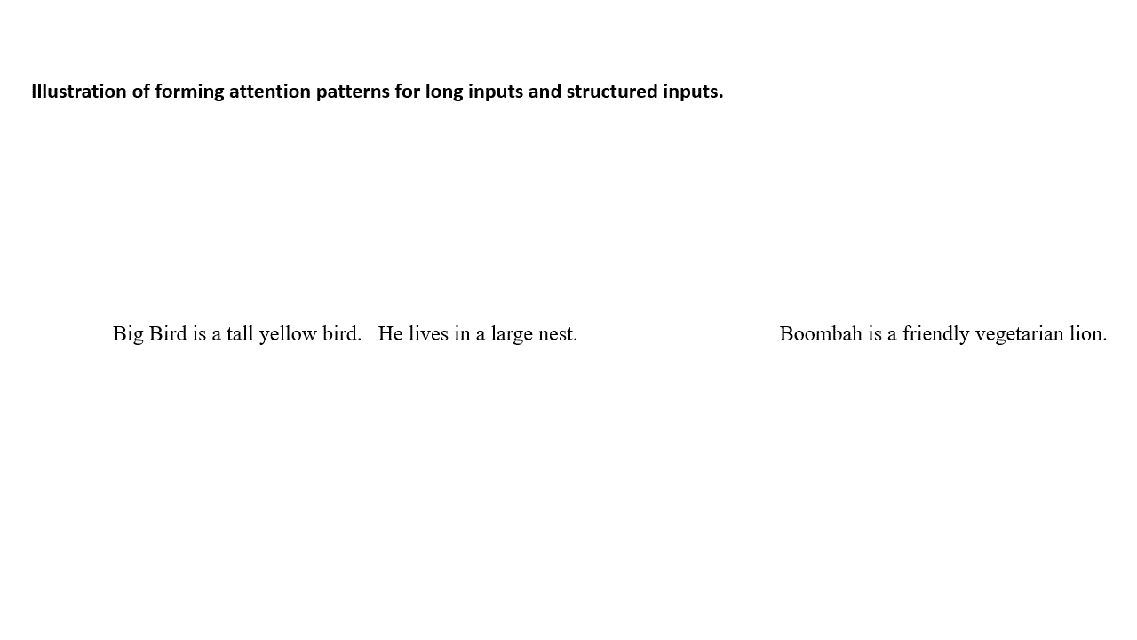
In order to further exploit the structure of long documents, ETC combines additional ideas: representing the positional information of the tokens in a relative way, rather than using their absolute position in the sequence; using an additional training objective beyond the usual masked language model (MLM) used in models like BERT; and flexible masking of tokens to control which tokens can attend to which other tokens. For example, given a long selection of text, a global token is applied to each sentence, which connects to all tokens within the sentence, and a global token is also applied to each paragraph, which connects to all tokens within the same paragraph.

An example of document structure based sparse attention of ETC model. The global variables are denoted by C (in blue) for paragraph, S (yellow) for sentence while the local variables are denoted by X (grey) for tokens corresponding to the long input.

With this approach, we report state-of-the-art results in five challenging NLP datasets requiring long or structured inputs: TriviaQA, Natural Questions (NQ), HotpotQA, WikiHop, and OpenKP.

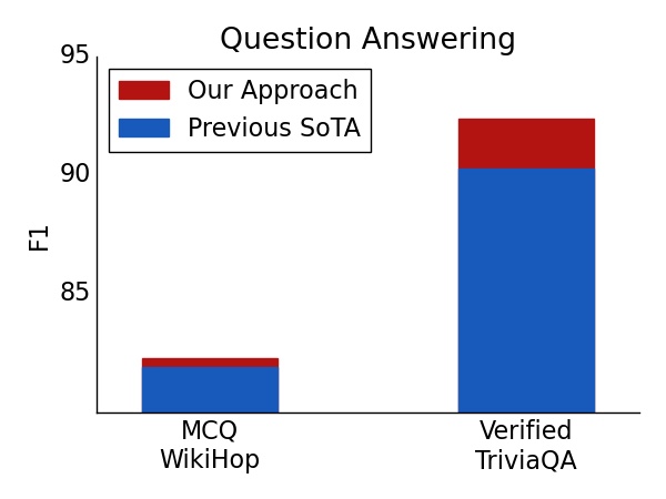
Test set result on Question Answering. For both verified TriviaQA and WikiHop, using ETC achieved a new state of the art.

BigBird
Extending the work of ETC, we propose BigBird — a sparse attention mechanism that is also linear in the number of tokens and is a generic replacement for the attention mechanism used in Transformers. In contrast to ETC, BigBird doesn’t require any prerequisite knowledge about structure present in the source data. Sparse attention in the BigBird model consists of three main parts:

  • A set of global tokens attending to all parts of the input sequence
  • All tokens attending to a set of local neighboring tokens
  • All tokens attending to a set of random tokens
BigBird sparse attention can be seen as adding few global tokens on Watts-Strogatz graph.

In the BigBird paper, we explain why sparse attention is sufficient to approximate quadratic attention, partially explaining why ETC was successful. A crucial observation is that there is an inherent tension between how few similarity scores one computes and the flow of information between different nodes (i.e., the ability of one token to influence each other). Global tokens serve as a conduit for information flow and we prove that sparse attention mechanisms with global tokens can be as powerful as the full attention model. In particular, we show that BigBird is as expressive as the original Transformer, is computationally universal (following the work of Yun et al. and Perez et al.), and is a universal approximator of continuous functions. Furthermore, our proof suggests that the use of random graphs can further help ease the flow of information — motivating the use of the random attention component.

This design scales to much longer sequence lengths for both structured and unstructured tasks. Further scaling can be achieved by using gradient checkpointing by trading off training time for sequence length. This lets us extend our efficient sparse transformers to include generative tasks that require an encoder and a decoder, such as long document summarization, on which we achieve a new state of the art.

Summarization ROUGE score for long documents. Both for BigPatent and ArXiv datasets, we achieve a new state of the art result.

Moreover, the fact that BigBird is a generic replacement also allows it to be extended to new domains without pre-existing domain knowledge. In particular, we introduce a novel application of Transformer-based models where long contexts are beneficial — extracting contextual representations of genomic sequences (DNA). With longer masked language model pre-training, BigBird achieves state-of-the-art performance on downstream tasks, such as promoter-region prediction and chromatin profile prediction.

On multiple genomics tasks, such as promoter region prediction (PRP), chromatin-profile prediction including transcription factors (TF), histone-mark (HM) and DNase I hypersensitive (DHS) detection, we outperform baselines. Moreover our results show that Transformer models can be applied to multiple genomics tasks that are currently underexplored.

Main Implementation Idea
One of the main impediments to the large scale adoption of sparse attention is the fact that sparse operations are quite inefficient in modern hardware. Behind both ETC and BigBird, one of our key innovations is to make an efficient implementation of the sparse attention mechanism. As modern hardware accelerators like GPUs and TPUs excel using coalesced memory operations, which load blocks of contiguous bytes at once, it is not efficient to have small sporadic look-ups caused by a sliding window (for local attention) or random element queries (random attention). Instead we transform the sparse local and random attention into dense tensor operations to take full advantage of modern single instruction, multiple data (SIMD) hardware.

To do this, we first “blockify” the attention mechanism to better leverage GPUs/TPUs, which are designed to operate on blocks. Then we convert the sparse attention mechanism computation into a dense tensor product through a series of simple matrix operations such as reshape, roll, and gather, as illustrated in the animation below.

Illustration of how sparse window attention is efficiently computed using roll and reshape, and without small sporadic look-ups.

Recently, “Long Range Arena: A Benchmark for Efficient Transformers“ provided a benchmark of six tasks that require longer context, and performed experiments to benchmark all existing long range transformers. The results show that the BigBird model, unlike its counterparts, clearly reduces memory consumption without sacrificing performance.

Conclusion
We show that carefully designed sparse attention can be as expressive and flexible as the original full attention model. Along with theoretical guarantees, we provide a very efficient implementation which allows us to scale to much longer inputs. As a consequence, we achieve state-of-the-art results for question answering, document summarization and genome fragment classification. Given the generic nature of our sparse attention, the approach should be applicable to many other tasks like program synthesis and long form open domain question answering. We have open sourced the code for both ETC (github) and BigBird (github), both of which run efficiently for long sequences on both GPUs and TPUs.

Acknowledgements
This research resulted as a collaboration with Amr Ahmed, Joshua Ainslie, Chris Alberti, Vaclav Cvicek, Avinava Dubey, Zachary Fisher, Guru Guruganesh, Santiago Ontañón, Philip Pham, Anirudh Ravula, Sumit Sanghai, Qifan Wang, Li Yang, Manzil Zaheer, who co-authored EMNLP and NeurIPS papers.

Source: Google AI Blog


LEAF: A Learnable Frontend for Audio Classification

Developing machine learning (ML) models for audio understanding has seen tremendous progress over the past several years. Leveraging the ability to learn parameters from data, the field has progressively shifted from composite, handcrafted systems to today’s deep neural classifiers that are used to recognize speech, understand music, or classify animal vocalizations such as bird calls. However, unlike computer vision models, which can learn from raw pixels, deep neural networks for audio classification are rarely trained from raw audio waveforms. Instead, they rely on pre-processed data in the form of mel filterbanks — handcrafted mel-scaled spectrograms that have been designed to replicate some aspects of the human auditory response.

Although modeling mel filterbanks for ML tasks has been historically successful, it is limited by the inherent biases of fixed features: even though using a fixed mel-scale and a logarithmic compression works well in general, we have no guarantee that they provide the best representations for the task at hand. In particular, even though matching human perception provides good inductive biases for some application domains, e.g., speech recognition or music understanding, these biases may be detrimental to domains for which imitating the human ear is not important, such as recognizing whale calls. So, in order to achieve optimal performance, the mel filterbanks should be tailored to the task of interest, a tedious process that requires an iterative effort informed by expert domain knowledge. As a consequence, standard mel filterbanks are used for most audio classification tasks in practice, even though they are suboptimal. In addition, while researchers have proposed ML systems to address these problems, such as Time-Domain Filterbanks, SincNet and Wavegram, they have yet to match the performance of traditional mel filterbanks.

In “LEAF, A Fully Learnable Frontend for Audio Classification”, accepted at ICLR 2021, we present an alternative method for crafting learnable spectrograms for audio understanding tasks. LEarnable Audio Frontend (LEAF) is a neural network that can be initialized to approximate mel filterbanks, and then be trained jointly with any audio classifier to adapt to the task at hand, while only adding a handful of parameters to the full model. We show that over a wide range of audio signals and classification tasks, including speech, music and bird songs, LEAF spectrograms improve classification performance over fixed mel filterbanks and over previously proposed learnable systems. We have implemented the code in TensorFlow 2 and released it to the community through our GitHub repository.

Mel Filterbanks: Mimicking Human Perception of Sound
The first step in the traditional approach to creating a mel filterbank is to capture the sound’s time-variability by windowing, i.e., cutting the signal into short segments with fixed duration. Then, one performs filtering, by passing the windowed segments through a bank of fixed frequency filters, that replicate the human logarithmic sensitivity to pitch. Because we are more sensitive to variations in low frequencies than high frequencies, mel filterbanks give more importance to the low-frequency range of sounds. Finally, the audio signal is compressed to mimic the ear’s logarithmic sensitivity to loudness — a sound needs to double its power for a person to perceive an increase of 3 decibels.

LEAF loosely follows this traditional approach to mel filterbank generation, but replaces each of the fixed operations (i.e., the filtering layer, windowing layer, and compression function) by a learned counterpart. The output of LEAF is a time-frequency representation (a spectrogram) similar to mel filterbanks, but fully learnable. So, for example, while a mel filterbank uses a fixed scale for pitch, LEAF learns the scale that is best suited to the task of interest. Any model that can be trained using mel filterbanks as input features, can also be trained on LEAF spectrograms.

Diagram of computation of mel filterbanks compared to LEAF spectrograms.

While LEAF can be initialized randomly, it can also be initialized in a way that approximates mel filterbanks, which have been shown to be a better starting point. Then, LEAF can be trained with any classifier to adapt to the task of interest.

Left: Mel filterbanks for a person saying “wow”. Right: LEAF’s output for the same example, after training on a dataset of speech commands.

A Parameter-Efficient Alternative to Fixed Features
A potential downside of replacing fixed features that involve no learnable parameter with a trainable system is that it can significantly increase the number of parameters to optimize. To avoid this issue, LEAF uses Gabor convolution layers that have only two parameters per filter, instead of the ~400 parameters typical of a standard convolution layer. This way, even when paired with a small classifier, such as EfficientNetB0, the LEAF model only accounts for 0.01% of the total parameters.

Top: Unconstrained convolutional filters after training for audio event classification. Bottom: LEAF filters at convergence after training for the same task.

Performance
We apply LEAF to diverse audio classification tasks, including recognizing speech commands, speaker identification, acoustic scene recognition, identifying musical instruments, and finding birdsongs. On average, LEAF outperforms both mel filterbanks and previous learnable frontends, such as Time-Domain Filterbanks, SincNet and Wavegram. In particular, LEAF achieves a 76.9% average accuracy across the different tasks, compared to 73.9% for mel filterbanks. Moreover we show that LEAF can be trained in a multi-task setting, such that a single LEAF parametrization can work well across all these tasks. Finally, when combined with a large audio classifier, LEAF reaches state-of-the-art performance on the challenging AudioSet benchmark, with a 2.74 d-prime score.

D-prime score (the higher the better) of LEAF, mel filterbanks and previously proposed learnable spectrograms on the evaluation set of AudioSet.

Conclusion
The scope of audio understanding tasks keeps growing, from diagnosing dementia from speech to detecting humpback whale calls from underwater microphones. Adapting mel filterbanks to every new task can require a significant amount of hand-tuning and experimentation. In this context, LEAF provides a drop-in replacement for these fixed features, that can be trained to adapt to the task of interest, with minimal task-specific adjustments. Thus, we believe that LEAF can accelerate development of models for new audio understanding tasks.

Acknowledgements
We thank our co-authors, Olivier Teboul, Félix de Chaumont-Quitry and Marco Tagliasacchi. We also thank Dick Lyon, Vincent Lostanlen, Matt Harvey, and Alex Park for helpful discussions, and Julie Thomas for helping to design figures for this post.

Source: Google AI Blog


A New Lens on Understanding Generalization in Deep Learning

Understanding generalization is one of the fundamental unsolved problems in deep learning. Why does optimizing a model on a finite set of training data lead to good performance on a held-out test set? This problem has been studied extensively in machine learning, with a rich history going back more than 50 years. There are now many mathematical tools that help researchers understand generalization in certain models. Unfortunately, most of these existing theories fail when applied to modern deep networks — they are both vacuous and non-predictive in realistic settings. This gap between theory and practice is largest for overparameterized models, which in theory have the capacity to overfit their train sets, but often do not in practice.

In “The Deep Bootstrap Framework: Good Online Learners are Good Offline Generalizers”, accepted at ICLR 2021, we present a new framework for approaching this problem by connecting generalization to the field of online optimization. In a typical setting, a model trains on a finite set of samples, which are reused for multiple epochs. But in online optimization, the model has access to an infinite stream of samples, and can be iteratively updated while processing this stream. In this work, we find that models that train quickly on infinite data are the same models that generalize well if they are instead trained on finite data. This connection brings new perspectives on design choices in practice, and lays a roadmap for understanding generalization from a theoretical perspective.

The Deep Bootstrap Framework
The main idea of the Deep Bootstrap framework is to compare the real world, where there is finite training data, to an "ideal world", where there is infinite data. We define these as:

  • Real World (N, T): Train a model on N train samples from a distribution, for T minibatch stochastic gradient descent (SGD) steps, re-using the same N samples in multiple epochs, as usual. This corresponds to running SGD on the empirical loss (loss on training data), and is the standard training procedure in supervised learning.
  • Ideal World (T): Train the same model for T steps, but use fresh samples from the distribution in each SGD step. That is, we run the exact same training code (same optimizer, learning-rates, batch-size, etc.), but sample a fresh train set in each epoch instead of reusing samples. In this ideal world setting, with an effectively infinite "train set", there is no difference between train error and test error.
Test soft-error for ideal world and real world during SGD iterations for ResNet-18 architecture. We see that the two errors are similar.

A priori, one might expect the real and ideal worlds may have nothing to do with each other, since in the real world the model sees a finite number of examples from the distribution while in the ideal world the model sees the whole distribution. But in practice, we found that the real and ideal models actually have similar test error.

In order to quantify this observation, we simulated an ideal world setting by creating a new dataset, which we call CIFAR-5m. We trained a generative model on CIFAR-10, which we then used to generate ~6 million images. The scale of the dataset was chosen to ensure that it is “virtually infinite” from the model’s perspective, so that the model never resamples the same data. That is, in the ideal world, the model sees an entirely fresh set of samples.

Samples from CIFAR-5m

The figure below presents the test error of several models, comparing their performance when trained on CIFAR-5m data in the real world setting (i.e., re-used data) and the ideal world (“fresh” data). The solid blue line shows a ResNet model in the real world, trained on 50K samples for 100 epochs with standard CIFAR-10 hyperparameters. The dashed blue line shows the corresponding model in the ideal world, trained on 5 million samples in a single pass. Surprisingly, these worlds have very similar test error — the model in some sense "doesn't care" whether it sees re-used samples or fresh ones.

The real world model is trained on 50K samples for 100 epochs, and the ideal world model is trained on 5M samples for a single epoch. The lines show the test error vs. the number of SGD steps.

This also holds for other architectures, e.g., a Multi-Layer-Perceptron (red), a Vision Transformer (green), and across many other settings of architecture, optimizer, data distribution, and sample size. These experiments suggest a new perspective on generalization: models that optimize quickly (on infinite data), generalize well (on finite data). For example, the ResNet model generalizes better than the MLP model on finite data, but this is "because" it optimizes faster even on infinite data.

Understanding Generalization from Optimization Behavior
The key observation is that real world and ideal world models remain close, in test error, for all timesteps, until the real world converges (< 1% train error). Thus, one can study models in the real world by studying their corresponding behavior in the ideal world.

This means that the generalization of the model can be understood in terms of its optimization performance under two frameworks:

  1. Online Optimization: How fast the ideal world test error decreases
  2. Offline Optimization: How fast the real world train error converges

Thus, to study generalization, we can equivalently study the two terms above, which can be conceptually simpler, since they only involve optimization concerns. Based on this observation, good models and training procedures are those that (1) optimize quickly in the ideal world and (2) do not optimize too quickly in the real world.

All design choices in deep learning can be viewed through their effect on these two terms. For example, some advances like convolutions, skip-connections, and pre-training help primarily by accelerating ideal world optimization, while other advances like regularization and data-augmentation help primarily by decelerating real world optimization.

Applying the Deep Bootstrap Framework
Researchers can use the Deep Bootstrap framework to study and guide design choices in deep learning. The principle is: whenever one makes a change that affects generalization in the real world (the architecture, learning-rate, etc.), one should consider its effect on (1) the ideal world optimization of test error (faster is better) and (2) the real world optimization of train error (slower is better).

For example, pre-training is often used in practice to help generalization of models in small-data regimes. However, the reason that pre-training helps remains poorly understood. One can study this using the Deep Bootstrap framework by looking at the effect of pre-training on terms (1) and (2) above. We find that the primary effect of pre-training is to improve the ideal world optimization (1) — pre-training turns the network into a "fast learner" for online optimization. The improved generalization of pretrained models is thus almost exactly captured by their improved optimization in the ideal world. The figure below shows this for Vision-Transformers (ViT) trained on CIFAR-10, comparing training from scratch vs. pre-training on ImageNet.

Effect of pre-training — pre-trained ViTs optimize faster in the ideal world.

One can also study data-augmentation using this framework. Data-augmentation in the ideal world corresponds to augmenting each fresh sample once, as opposed to augmenting the same sample multiple times. This framework implies that good data-augmentations are those that (1) do not significantly harm ideal world optimization (i.e., augmented samples don't look too "out of distribution") or (2) inhibit real world optimization speed (so the real world takes longer to fit its train set).

The main benefit of data-augmentation is through the second term, prolonging the real world optimization time. As for the first term, some aggressive data augmentations (mixup/cutout) can actually harm the ideal world, but this effect is dwarfed by the second term.

Concluding Thoughts
The Deep Bootstrap framework provides a new lens on generalization and empirical phenomena in deep learning. We are excited to see it applied to understand other aspects of deep learning in the future. It is especially interesting that generalization can be characterized via purely optimization considerations, which is in contrast to many prevailing approaches in theory. Crucially, we consider both online and offline optimization, which are individually insufficient, but that together determine generalization.

The Deep Bootstrap framework can also shed light on why deep learning is fairly robust to many design choices: many kinds of architectures, loss functions, optimizers, normalizations, and activation functions can generalize well. This framework suggests a unifying principle: that essentially any choice that works well in the online optimization setting will also generalize well in the offline setting.

Finally, modern neural networks can be either overparameterized (e.g., large networks trained on small data tasks) or underparmeterized (e.g., OpenAI's GPT-3, Google's T5, or Facebook's ResNeXt WSL). The Deep Bootstrap framework implies that online optimization is a crucial factor to success in both regimes.

Acknowledgements
We are thankful to our co-author, Behnam Neyshabur, for his great contributions to the paper and valuable feedback on the blog. We thank Boaz Barak, Chenyang Yuan, and Chiyuan Zhang for helpful comments on the blog and paper.

Source: Google AI Blog


Accelerating Neural Networks on Mobile and Web with Sparse Inference

On-device inference of neural networks enables a variety of real-time applications, like pose estimation and background blur, in a low-latency and privacy-conscious way. Using ML inference frameworks like TensorFlow Lite with XNNPACK ML acceleration library, engineers optimize their models to run on a variety of devices by finding a sweet spot between model size, inference speed and the quality of the predictions.

One way to optimize a model is through use of sparse neural networks [1, 2, 3], which have a significant fraction of their weights set to zero. In general, this is a desirable quality as it not only reduces the model size via compression, but also makes it possible to skip a significant fraction of multiply-add operations, thereby speeding up inference. Further, it is possible to increase the number of parameters in a model and then sparsify it to match the quality of the original model, while still benefiting from the accelerated inference. However, the use of this technique remains limited in production largely due to a lack of tools to sparsify popular convolutional architectures as well as insufficient support for running these operations on-device.

Today we announce the release of a set of new features for the XNNPACK acceleration library and TensorFlow Lite that enable efficient inference of sparse networks, along with guidelines on how to sparsify neural networks, with the goal of helping researchers develop their own sparse on-device models. Developed in collaboration with DeepMind, these tools power a new generation of live perception experiences, including hand tracking in MediaPipe and background features in Google Meet, accelerating inference speed from 1.2 to 2.4 times, while reducing the model size by half. In this post, we provide a technical overview of sparse neural networks — from inducing sparsity during training to on-device deployment — and offer some ideas on how researchers might create their own sparse models.

Comparison of the processing time for the dense (left) and sparse (right) models of the same quality for Google Meet background features. For readability, the processing time shown is the moving average across 100 frames.

Sparsifying a Neural Network
Many modern deep learning architectures, like MobileNet and EfficientNetLite, are primarily composed of depthwise convolutions with a small spatial kernel and 1x1 convolutions that linearly combine features from the input image. While such architectures have a number of potential targets for sparsification, including the full 2D convolutions that frequently occur at the beginning of many networks or the depthwise convolutions, it is the 1x1 convolutions that are the most expensive operators as measured by inference time. Because they account for over 65% of the total compute, they are an optimal target for sparsification.

Architecture Inference Time
MobileNet 85%
MobileNetV2 71%
MobileNetV3 71%
EfficientNet-Lite   66%
Comparison of inference time dedicated to 1x1 convolutions in % for modern mobile architectures.

In modern on-device inference engines, like XNNPACK, the implementation of 1x1 convolutions as well as other operations in the deep learning models rely on the HWC tensor layout, in which the tensor dimensions correspond to the height, width, and channel (e.g., red, green or blue) of the input image. This tensor configuration allows the inference engine to process the channels corresponding to each spatial location (i.e., each pixel of an image) in parallel. However, this ordering of the tensor is not a good fit for sparse inference because it sets the channel as the innermost dimension of the tensor and makes it more computationally expensive to access.

Our updates to XNNPACK enable it to detect if a model is sparse. If so, it switches from its standard dense inference mode to sparse inference mode, in which it employs a CHW (channel, height, width) tensor layout. This reordering of the tensor allows for an accelerated implementation of the sparse 1x1 convolution kernel for two reasons: 1) entire spatial slices of the tensor can be skipped when the corresponding channel weight is zero following a single condition check, instead of a per-pixel test; and 2) when the channel weight is non-zero, the computation can be made more efficient by loading neighbouring pixels into the same memory unit. This enables us to process multiple pixels simultaneously, while also performing each operation in parallel across several threads. Together these changes result in a speed-up of 1.8x to 2.3x when at least 80% of the weights are zero.

In order to avoid converting back and forth between the CHW tensor layout that is optimal for sparse inference and the standard HWC tensor layout after each operation, XNNPACK provides efficient implementations of several CNN operators in CHW layout.

Guidelines for Training Sparse Neural Networks
To create a sparse neural network, the guidelines included in this release suggest one start with a dense version and then gradually set a fraction of its weights to zero during training. This process is called pruning. Of the many available techniques for pruning, we recommend using magnitude pruning (available in the TF Model Optimization Toolkit) or the recently introduced RigL method. With a modest increase in training time, both of these can successfully sparsify deep learning models without degrading their quality. The resulting sparse models can be stored efficiently in a compressed format that reduces the size by a factor of two compared to their dense equivalent.

The quality of sparse networks is influenced by several hyperparameters, including training time, learning rate and schedules for pruning. The TF Pruning API provides an excellent example of how to select these, as well as some tips for training such models. We recommend running hyperparameter searches to find the sweet spot for your application.

Applications
We demonstrate that it is possible to sparsify classification tasks, dense segmentation (e.g., Meet background blur) and regression problems (MediaPipe Hands), which provides tangible benefits to users. For example, in the case of Google Meet, sparsification lowered the inference time of the model by 30%, which provided access to higher quality models for more users.

Model size comparisons for the dense and sparse models in Mb. The models have been stored in 16- and 32-bit floating-point formats.

The approach to sparsity described here works best with architectures based on inverted residual blocks, such as MobileNetV2, MobileNetV3 and EfficientNetLite. The degree of sparsity in a network influences both inference speed and quality. Starting from a dense network of a fixed capacity, we found modest performance gains even at 30% sparsity. With increased sparsity, the quality of the model remains relatively close to the dense baseline until reaching 70% sparsity, beyond which there is a more pronounced drop in accuracy. However, one can compensate for the reduced accuracy at 70% sparsity by increasing the size of the base network by 20%, which results in faster inference times without degrading the quality of the model. No further changes are required to run the sparsified models, because XNNPACK can recognize and automatically enable sparse inference.

Ablation studies of different sparsity levels with respect to inference time (the smaller the better) and the quality measured by the Intersection over Union (IoU) for predicted segmentation mask.

Sparsity as Automatic Alternative to Distillation
Background blur in Google Meet uses a segmentation model based on a modified MobileNetV3 backbone with attention blocks. We were able to speed up the model by 30% by applying a 70% sparsification, while preserving the quality of the foreground mask. We examined the predictions of the sparse and dense models on images from 17 geographic subregions, finding no significant difference, and released the details in the associated model card.

Similarly, MediaPipe Hands predicts hand landmarks in real-time on mobile and the web using a model based on the EfficientNetLite backbone. This backbone model was manually distilled from the large dense model, which is a computationally expensive, iterative process. Using the sparse version of the dense model instead of distilled one, we were able to maintain the same inference speed but without the labor intensive process of distilling from a dense model. Compared with the dense model the sparse model improved the inference by a factor of two, achieving the identical landmark quality as the distilled model. In a sense, sparsification can be thought of as an automatic approach to unstructured model distillation, which can improve model performance without extensive manual effort. We evaluated the sparse model on the geodiverse dataset and made the model card publicly available.

Comparison of execution time for the dense (left), distilled (middle) and sparse (right) models of the same quality. Processing time of the dense model is 2x larger than sparse or distilled models. The distilled model is taken from the official MediPipe solution. The dense and sparse web demos are publicly available.

Future work
We find sparsification to be a simple yet powerful technique for improving CPU inference of neural networks. Sparse inference allows engineers to run larger models without incurring a significant performance or size overhead and offers a promising new direction for research. We are continuing to extend XNNPACK with wider support for operations in CHW layout and are exploring how it might be combined with other optimization techniques like quantization. We are excited to see what you might build with this technology!

Acknowledgments
Special thanks to all who worked on this project: Karthik Raveendran, Erich Elsen, Tingbo Hou‎, Trevor Gale, Siargey Pisarchyk, Yury Kartynnik, Yunlu Li, Utku Evci, Matsvei Zhdanovich, Sebastian Jansson, Stéphane Hulaud, Michael Hays, Juhyun Lee, Fan Zhang, Chuo-Ling Chang, Gregory Karpiak, Tyler Mullen, Jiuqiang Tang, Ming Guang Yong, Igor Kibalchich, and Matthias Grundmann.

Source: Google AI Blog


PAIRED: A New Multi-agent Approach for Adversarial Environment Generation

The effectiveness of any machine learning method is critically dependent on its training data. In the case of reinforcement learning (RL), one can rely either on limited data collected by an agent interacting with the real world, or a simulated training environment that can be used to collect as much data as needed. This latter method of training in simulation is increasingly popular, but it has a problem — the RL agent can learn what is built into the simulator, but tends to be bad at generalizing to tasks that are even slightly different than the ones simulated. And obviously building a simulator that covers all the complexity of the real-world is extremely challenging.

An approach to address this is to automatically create more diverse training environments by randomizing all the parameters of the simulator, a process called domain randomization (DR). However, DR can fail even in very simple environments. For example, in the animation below, the blue agent is trying to navigate to the green goal. The left panel shows an environment created with DR where the positions of the obstacles and goal have been randomized. Many of these DR environments were used to train the agent, which was then transferred to the simple Four Rooms environment in the middle panel. Notice that the agent can’t find the goal. This is because it has not learned to walk around walls. Even though the wall configuration from the Four Rooms example could have been generated randomly in the DR training phase, it’s unlikely. As a result, the agent has not spent enough time training on walls similar to the Four Rooms structure, and is unable to reach the goal.

Domain randomization (left) does not effectively prepare an agent to transfer to previously unseen environments, such as the Four Rooms scenario (middle). To address this, a minimax adversary is used to construct previously unseen environments (right), but can result in creating situations that are impossible to solve.

Instead of just randomizing the environment parameters, one could train a second RL agent to learn how to set the environment parameters. This minimax adversary can be trained to minimize the performance of the first RL agent by finding and exploiting weaknesses in its policy - e.g. building wall configurations it has not encountered before. But again there is a problem. The right panel shows an environment built by a minimax adversary in which it is actually impossible for the agent to reach the goal. While the minimax adversary has succeeded in its task — it has minimized the performance of the original agent — it provides no opportunity for the agent to learn. Using a purely adversarial objective is not well suited to generating training environments, either.

In collaboration with UC Berkeley, we propose a new multi-agent approach for training the adversary in “Emergent Complexity and Zero-shot Transfer via Unsupervised Environment Design”, a publication recently presented at NeurIPS 2020. In this work we present an algorithm, Protagonist Antagonist Induced Regret Environment Design (PAIRED), that is based on minimax regret and prevents the adversary from creating impossible environments, while still enabling it to correct weaknesses in the agent’s policy. PAIRED incentivizes the adversary to tune the difficulty of the generated environments to be just outside the agent’s current abilities, leading to an automatic curriculum of increasingly challenging training tasks. We show that agents trained with PAIRED learn more complex behavior and generalize better to unknown test tasks. We have released open-source code for PAIRED on our GitHub repo.

PAIRED
To flexibly constrain the adversary, PAIRED introduces a third RL agent, which we call the antagonist agent, because it is allied with the adversarial agent, i.e., the one designing the environment. We rename our initial agent, the one navigating the environment, the protagonist. Once the adversary generates an environment, both the protagonist and antagonist play through that environment.

The adversary’s job is to maximize the antagonist’s reward while minimizing the protagonist's reward. This means it must create environments that are feasible (because the antagonist can solve them and get a high score), but challenging to the protagonist (exploit weaknesses in its current policy). The gap between the two rewards is the regret — the adversary tries to maximize the regret, while the protagonist competes to minimize it.

The methods discussed above (domain randomization, minimax regret and PAIRED) can be analyzed using the same theoretical framework, unsupervised environment design (UED), which we describe in detail in the paper. UED draws a connection between environment design and decision theory, enabling us to show that domain randomization is equivalent to the Principle of Insufficient Reason, the minimax adversary follows the Maximin Principle, and PAIRED is optimizing minimax regret. Below, we show how each of these ideas works for environment design:

Domain randomization (a) generates unstructured environments that aren’t tailored to the agent’s learning progress. The minimax adversary (b) may create impossible environments. PAIRED (c) can generate challenging, structured environments, which are still possible for the agent to complete.

Curriculum Generation
What’s interesting about minimax regret is that it incentivizes the adversary to generate a curriculum of initially easy, then increasingly challenging environments. In most RL environments, the reward function will give a higher score for completing the task more efficiently, or in fewer timesteps. When this is true, we can show that regret incentivizes the adversary to create the easiest possible environment the protagonist can’t solve yet. To see this, let’s assume the antagonist is perfect, and always gets the highest score that it possibly can. Meanwhile, the protagonist is terrible, and gets a score of zero on everything. In that case, the regret just depends on the difficulty of the environment. Since easier environments can be completed in fewer timesteps, they allow the antagonist to get a higher score. Therefore, the regret of failing at an easy environment is greater than the regret of failing on a hard environment:

So, by maximizing regret the adversary is searching for easy environments that the protagonist fails to do. Once the protagonist learns to solve each environment, the adversary must move on to finding a slightly harder environment that the protagonist can’t solve. Thus, the adversary generates a curriculum of increasingly difficult tasks.

Results
We can see the curriculum emerging in the learning curves below, which plot the shortest path length of a maze the agents have successfully solved. Unlike minimax or domain randomization, the PAIRED adversary creates a curriculum of increasingly longer, but possible, mazes, enabling PAIRED agents to learn more complex behavior.

But can these different training schemes help an agent generalize better to unknown test tasks? Below, we see the zero-shot transfer performance of each algorithm on a series of challenging test tasks. As the complexity of the transfer environment increases, the performance gap between PAIRED and the baselines widens. For extremely difficult tasks like Labyrinth and Maze, PAIRED is the only method that can occasionally solve the task. These results provide promising evidence that PAIRED can be used to improve generalization for deep RL.

Admittedly, these simple gridworlds do not reflect the complexities of the real world tasks that many RL methods are attempting to solve. We address this in “Adversarial Environment Generation for Learning to Navigate the Web”, which examines the performance of PAIRED when applied to more complex problems, such as teaching RL agents to navigate web pages. We propose an improved version of PAIRED, and show how it can be used to train an adversary to generate a curriculum of increasingly challenging websites:

Above, you can see websites built by the adversary in the early, middle, and late training stages, which progress from using very few elements per page to many simultaneous elements, making the tasks progressively harder. We test whether agents trained on this curriculum can generalize to standardized web navigation tasks, and achieve a 75% success rate, with a 4x improvement over the strongest curriculum learning baseline:

Conclusions
Deep RL is very good at fitting a simulated training environment, but how can we build simulations that cover the complexity of the real world? One solution is to automate this process. We propose Unsupervised Environment Design (UED) as a framework that describes different methods for automatically creating a distribution of training environments, and show that UED subsumes prior work like domain randomization and minimax adversarial training. We think PAIRED is a good approach for UED, because regret maximization leads to a curriculum of increasingly challenging tasks, and prepares agents to transfer successfully to unknown test tasks.

Acknowledgements
We would like to recognize the co-authors of “Emergent Complexity and Zero-shot Transfer via Unsupervised Environment Design”: Michael Dennis, Natasha Jaques, Eugene Vinitsky, Alexandre Bayen, Stuart Russell, Andrew Critch, and Sergey Levine, as well as the co-authors of Adversarial Environment Generation for Learning to Navigate the Web: Izzeddin Gur, Natasha Jaques, Yingjie Miao, Jongwook Choi, Kevin Malta, Manoj Tiwari, Honglak Lee, Aleksandra Faust. In addition, we thank Michael Chang, Marvin Zhang, Dale Schuurmans, Aleksandra Faust, Chase Kew, Jie Tan, Dennis Lee, Kelvin Xu, Abhishek Gupta, Adam Gleave, Rohin Shah, Daniel Filan, Lawrence Chan, Sam Toyer, Tyler Westenbroek, Igor Mordatch, Shane Gu, DJ Strouse, and Max Kleiman-Weiner for discussions that contributed to this work.

Source: Google AI Blog


The Technology Behind Cinematic Photos

Looking at photos from the past can help people relive some of their most treasured moments. Last December we launched Cinematic photos, a new feature in Google Photos that aims to recapture the sense of immersion felt the moment a photo was taken, simulating camera motion and parallax by inferring 3D representations in an image. In this post, we take a look at the technology behind this process, and demonstrate how Cinematic photos can turn a single 2D photo from the past into a more immersive 3D animation.

Camera 3D model courtesy of Rick Reitano.
Depth Estimation
Like many recent computational photography features such as Portrait Mode and Augmented Reality (AR), Cinematic photos requires a depth map to provide information about the 3D structure of a scene. Typical techniques for computing depth on a smartphone rely on multi-view stereo, a geometry method to solve for the depth of objects in a scene by simultaneously capturing multiple photos at different viewpoints, where the distances between the cameras is known. In the Pixel phones, the views come from two cameras or dual-pixel sensors.

To enable Cinematic photos on existing pictures that were not taken in multi-view stereo, we trained a convolutional neural network with encoder-decoder architecture to predict a depth map from just a single RGB image. Using only one view, the model learned to estimate depth using monocular cues, such as the relative sizes of objects, linear perspective, defocus blur, etc.

Because monocular depth estimation datasets are typically designed for domains such as AR, robotics, and self-driving, they tend to emphasize street scenes or indoor room scenes instead of features more common in casual photography, like people, pets, and objects, which have different composition and framing. So, we created our own dataset for training the monocular depth model using photos captured on a custom 5-camera rig as well as another dataset of Portrait photos captured on Pixel 4. Both datasets included ground-truth depth from multi-view stereo that is critical for training a model.

Mixing several datasets in this way exposes the model to a larger variety of scenes and camera hardware, improving its predictions on photos in the wild. However, it also introduces new challenges, because the ground-truth depth from different datasets may differ from each other by an unknown scaling factor and shift. Fortunately, the Cinematic photo effect only needs the relative depths of objects in the scene, not the absolute depths. Thus we can combine datasets by using a scale-and-shift-invariant loss during training and then normalize the output of the model at inference.

The Cinematic photo effect is particularly sensitive to the depth map’s accuracy at person boundaries. An error in the depth map can result in jarring artifacts in the final rendered effect. To mitigate this, we apply median filtering to improve the edges, and also infer segmentation masks of any people in the photo using a DeepLab segmentation model trained on the Open Images dataset. The masks are used to pull forward pixels of the depth map that were incorrectly predicted to be in the background.

Camera Trajectory
There can be many degrees of freedom when animating a camera in a 3D scene, and our virtual camera setup is inspired by professional video camera rigs to create cinematic motion. Part of this is identifying the optimal pivot point for the virtual camera’s rotation in order to yield the best results by drawing one’s eye to the subject.

The first step in 3D scene reconstruction is to create a mesh by extruding the RGB image onto the depth map. By doing so, neighboring points in the mesh can have large depth differences. While this is not noticeable from the “face-on” view, the more the virtual camera is moved, the more likely it is to see polygons spanning large changes in depth. In the rendered output video, this will look like the input texture is stretched. The biggest challenge when animating the virtual camera is to find a trajectory that introduces parallax while minimizing these “stretchy” artifacts.

The parts of the mesh with large depth differences become more visible (red visualization) once the camera is away from the “face-on” view. In these areas, the photo appears to be stretched, which we call “stretchy artifacts”.

Because of the wide spectrum in user photos and their corresponding 3D reconstructions, it is not possible to share one trajectory across all animations. Instead, we define a loss function that captures how much of the stretchiness can be seen in the final animation, which allows us to optimize the camera parameters for each unique photo. Rather than counting the total number of pixels identified as artifacts, the loss function triggers more heavily in areas with a greater number of connected artifact pixels, which reflects a viewer’s tendency to more easily notice artifacts in these connected areas.

We utilize padded segmentation masks from a human pose network to divide the image into three different regions: head, body and background. The loss function is normalized inside each region before computing the final loss as a weighted sum of the normalized losses. Ideally the generated output video is free from artifacts but in practice, this is rare. Weighting the regions differently biases the optimization process to pick trajectories that prefer artifacts in the background regions, rather than those artifacts near the image subject.

During the camera trajectory optimization, the goal is to select a path for the camera with the least amount of noticeable artifacts. In these preview images, artifacts in the output are colored red while the green and blue overlay visualizes the different body regions.

Framing the Scene
Generally, the reprojected 3D scene does not neatly fit into a rectangle with portrait orientation, so it was also necessary to frame the output with the correct right aspect ratio while still retaining the key parts of the input image. To accomplish this, we use a deep neural network that predicts per-pixel saliency of the full image. When framing the virtual camera in 3D, the model identifies and captures as many salient regions as possible while ensuring that the rendered mesh fully occupies every output video frame. This sometimes requires the model to shrink the camera's field of view.

Heatmap of the predicted per-pixel saliency. We want the creation to include as much of the salient regions as possible when framing the virtual camera.

Conclusion
Through Cinematic photos, we implemented a system of algorithms – with each ML model evaluated for fairness – that work together to allow users to relive their memories in a new way, and we are excited about future research and feature improvements. Now that you know how they are created, keep an eye open for automatically created Cinematic photos that may appear in your recent memories within the Google Photos app!

Acknowledgments
Cinematic Photos is the result of a collaboration between Google Research and Google Photos teams. Key contributors also include: Andre Le, Brian Curless, Cassidy Curtis, Ce Liu‎, Chun-po Wang, Daniel Jenstad, David Salesin, Dominik Kaeser, Gina Reynolds, Hao Xu, Huiwen Chang, Huizhong Chen‎, Jamie Aspinall, Janne Kontkanen, Matthew DuVall, Michael Kucera, Michael Milne, Mike Krainin, Mike Liu, Navin Sarma, Orly Liba, Peter Hedman, Rocky Cai‎, Ruirui Jiang‎, Steven Hickson, Tracy Gu, Tyler Zhu, Varun Jampani, Yuan Hao, Zhongli Ding.

Source: Google AI Blog


Introducing Model Search: An Open Source Platform for Finding Optimal ML Models

The success of a neural network (NN) often depends on how well it can generalize to various tasks. However, designing NNs that can generalize well is challenging because the research community's understanding of how a neural network generalizes is currently somewhat limited: What does the appropriate neural network look like for a given problem? How deep should it be? Which types of layers should be used? Would LSTMs be enough or would Transformer layers be better? Or maybe a combination of the two? Would ensembling or distillation boost performance? These tricky questions are made even more challenging when considering machine learning (ML) domains where there may exist better intuition and deeper understanding than others.

In recent years, AutoML algorithms have emerged [e.g., 1, 2, 3] to help researchers find the right neural network automatically without the need for manual experimentation. Techniques like neural architecture search (NAS), use algorithms, like reinforcement learning (RL), evolutionary algorithms, and combinatorial search, to build a neural network out of a given search space. With the proper setup, these techniques have demonstrated they are capable of delivering results that are better than the manually designed counterparts. But more often than not, these algorithms are compute heavy, and need thousands of models to train before converging. Moreover, they explore search spaces that are domain specific and incorporate substantial prior human knowledge that does not transfer well across domains. As an example, in image classification, the traditional NAS searches for two good building blocks (convolutional and downsampling blocks), that it arranges following traditional conventions to create the full network.

To overcome these shortcomings and to extend access to AutoML solutions to the broader research community, we are excited to announce the open source release of Model Search, a platform that helps researchers develop the best ML models, efficiently and automatically. Instead of focusing on a specific domain, Model Search is domain agnostic, flexible and is capable of finding the appropriate architecture that best fits a given dataset and problem, while minimizing coding time, effort and compute resources. It is built on Tensorflow, and can run either on a single machine or in a distributed setting.

Overview
The Model Search system consists of multiple trainers, a search algorithm, a transfer learning algorithm and a database to store the various evaluated models. The system runs both training and evaluation experiments for various ML models (different architectures and training techniques) in an adaptive, yet asynchronous, fashion. While each trainer conducts experiments independently, all trainers share the knowledge gained from their experiments. At the beginning of every cycle, the search algorithm looks up all the completed trials and uses beam search to decide what to try next. It then invokes mutation over one of the best architectures found thus far and assigns the resulting model back to a trainer.

Model Search schematic illustrating the distributed search and ensembling. Each trainer runs independently to train and evaluate a given model. The results are shared with the search algorithm, which it stores. The search algorithm then invokes mutation over one of the best architectures and then sends the new model back to a trainer for the next iteration. S is the set of training and validation examples and A are all the candidates used during training and search.

The system builds a neural network model from a set of predefined blocks, each of which represents a known micro-architecture, like LSTM, ResNet or Transformer layers. By using blocks of pre-existing architectural components, Model Search is able to leverage existing best knowledge from NAS research across domains. This approach is also more efficient, because it explores structures, not their more fundamental and detailed components, therefore reducing the scale of the search space.

Neural network micro architecture blocks that work well, e.g., a ResNet Block.

Because the Model Search framework is built on Tensorflow, blocks can implement any function that takes a tensor as an input. For example, imagine that one wants to introduce a new search space built with a selection of micro architectures. The framework will take the newly defined blocks and incorporate them into the search process so that algorithms can build the best possible neural network from the components provided. The blocks provided can even be fully defined neural networks that are already known to work for the problem of interest. In that case, Model Search can be configured to simply act as a powerful ensembling machine.

The search algorithms implemented in Model Search are adaptive, greedy and incremental, which makes them converge faster than RL algorithms. They do however imitate the “explore & exploit” nature of RL algorithms by separating the search for a good candidate (explore step), and boosting accuracy by ensembling good candidates that were discovered (exploit step). The main search algorithm adaptively modifies one of the top k performing experiments (where k can be specified by the user) after applying random changes to the architecture or the training technique (e.g., making the architecture deeper).

An example of an evolution of a network over many experiments. Each color represents a different type of architecture block. The final network is formed via mutations of high performing candidate networks, in this case adding depth.

To further improve efficiency and accuracy, transfer learning is enabled between various internal experiments. Model Search does this in two ways — via knowledge distillation or weight sharing. Knowledge distillation allows one to improve candidates' accuracies by adding a loss term that matches the high performing models’ predictions in addition to the ground truth. Weight sharing, on the other hand, bootstraps some of the parameters (after applying mutation) in the network from previously trained candidates by copying suitable weights from previously trained models and randomly initializing the remaining ones. This enables faster training, which allows opportunities to discover more (and better) architectures.

Experimental Results
Model Search improves upon production models with minimal iterations. In a recent paper, we demonstrated the capabilities of Model Search in the speech domain by discovering a model for keyword spotting and language identification. Over fewer than 200 iterations, the resulting model slightly improved upon internal state-of-the-art production models designed by experts in accuracy using ~130K fewer trainable parameters (184K compared to 315K parameters).

Model accuracy given iteration in our system compared to the previous production model for keyword spotting, a similar graph can be found for language identification in the linked paper.

We also applied Model Search to find an architecture suitable for image classification on the heavily explored CIFAR-10 imaging dataset. Using a set known convolution blocks, including convolutions, resnet blocks (i.e., two convolutions and a skip connection), NAS-A cells, fully connected layers, etc., we observed that we were able to quickly reach a benchmark accuracy of 91.83 in 209 trials (i.e., exploring only 209 models). In comparison, previous top performers reached the same threshold accuracy in 5807 trials for the NasNet algorithm (RL), and 1160 for PNAS (RL + Progressive).

Conclusion
We hope the Model Search code will provide researchers with a flexible, domain-agnostic framework for ML model discovery. By building upon previous knowledge for a given domain, we believe that this framework is powerful enough to build models with the state-of-the-art performance on well studied problems when provided with a search space composed of standard building blocks.

Acknowledgements
Special thanks to all code contributors to the open sourcing and the paper: Eugen Ehotaj, Scotty Yak, Malaika Handa, James Preiss, Pai Zhu, Aleks Kracun, Prashant Sridhar, Niranjan Subrahmanya, Ignacio Lopez Moreno, Hyun Jin Park, and Patrick Violette.

Source: Google AI Blog


MediaPipe Holistic — Simultaneous Face, Hand and Pose Prediction, on Device

Real-time, simultaneous perception of human pose, face landmarks and hand tracking on mobile devices can enable a variety of impactful applications, such as fitness and sport analysis, gesture control and sign language recognition, augmented reality effects and more. MediaPipe, an open-source framework designed specifically for complex perception pipelines leveraging accelerated inference (e.g., GPU or CPU), already offers fast and accurate, yet separate, solutions for these tasks. Combining them all in real-time into a semantically consistent end-to-end solution is a uniquely difficult problem requiring simultaneous inference of multiple, dependent neural networks.

Today, we are excited to announce MediaPipe Holistic, a solution to this challenge that provides a novel state-of-the-art human pose topology that unlocks novel use cases. MediaPipe Holistic consists of a new pipeline with optimized pose, face and hand components that each run in real-time, with minimum memory transfer between their inference backends, and added support for interchangeability of the three components, depending on the quality/speed tradeoffs. When including all three components, MediaPipe Holistic provides a unified topology for a groundbreaking 540+ keypoints (33 pose, 21 per-hand and 468 facial landmarks) and achieves near real-time performance on mobile devices. MediaPipe Holistic is being released as part of MediaPipe and is available on-device for mobile (Android, iOS) and desktop. We are also introducing MediaPipe’s new ready-to-use APIs for research (Python) and web (JavaScript) to ease access to the technology.

Top: MediaPipe Holistic results on sport and dance use-cases. Bottom: “Silence” and “Hello” gestures. Note, that our solution consistently identifies a hand as either right (blue color) or left (orange color).

Pipeline and Quality
The MediaPipe Holistic pipeline integrates separate models for pose, face and hand components, each of which are optimized for their particular domain. However, because of their different specializations, the input to one component is not well-suited for the others. The pose estimation model, for example, takes a lower, fixed resolution video frame (256x256) as input. But if one were to crop the hand and face regions from that image to pass to their respective models, the image resolution would be too low for accurate articulation. Therefore, we designed MediaPipe Holistic as a multi-stage pipeline, which treats the different regions using a region appropriate image resolution.

First, MediaPipe Holistic estimates the human pose with BlazePose’s pose detector and subsequent keypoint model. Then, using the inferred pose key points, it derives three regions of interest (ROI) crops for each hand (2x) and the face, and employs a re-crop model to improve the ROI (details below). The pipeline then crops the full-resolution input frame to these ROIs and applies task-specific face and hand models to estimate their corresponding keypoints. Finally, all key points are merged with those of the pose model to yield the full 540+ keypoints.

MediaPipe Holistic pipeline overview.

To streamline the identification of ROIs, a tracking approach similar to the one used for the standalone face and hand pipelines is utilized. This approach assumes that the object doesn't move significantly between frames, using an estimation from the previous frame as a guide to the object region in the current one. However, during fast movements, the tracker can lose the target, which requires the detector to re-localize it in the image. MediaPipe Holistic uses pose prediction (on every frame) as an additional ROI prior to reduce the response time of the pipeline when reacting to fast movements. This also enables the model to retain semantic consistency across the body and its parts by preventing a mixup between left and right hands or body parts of one person in the frame with another.

In addition, the resolution of the input frame to the pose model is low enough that the resulting ROIs for face and hands are still too inaccurate to guide the re-cropping of those regions, which require a precise input crop to remain lightweight. To close this accuracy gap we use lightweight face and hand re-crop models that play the role of spatial transformers and cost only ~10% of the corresponding model's inference time.

 MEH   FLE 
 Tracking pipeline (baseline)   9.8%   3.1% 
 Pipeline without re-crops   11.8%   3.5% 
 Pipeline with re-crops   9.7%   3.1% 
Hand prediction quality.The mean error per hand (MEH) is normalized by the hand size. The face landmarks error (FLE) is normalized by the inter-pupillary distance.

Performance
MediaPipe Holistic requires coordination between up to 8 models per frame — 1 pose detector, 1 pose landmark model, 3 re-crop models and 3 keypoint models for hands and face. While building this solution, we optimized not only machine learning models, but also pre- and post-processing algorithms (e.g., affine transformations), which take significant time on most devices due to pipeline complexity. In this case, moving all the pre-processing computations to GPU resulted in ~1.5 times overall pipeline speedup depending on the device. As a result, MediaPipe Holistic runs in near real-time performance even on mid-tier devices and in the browser.

 Phone   FPS 
 Google Pixel 2 XL   18 
 Samsung S9+   20 
 15-inch MacBook Pro 2017   15 
Performance on various mid-tier devices, measured in frames per second (FPS) using TFLite GPU.

The multi-stage nature of the pipeline provides two more performance benefits. As models are mostly independent, they can be replaced with lighter or heavier versions (or turned off completely) depending on the performance and accuracy requirements. Also, once pose is inferred, one knows precisely whether hands and face are within the frame bounds, allowing the pipeline to skip inference on those body parts.

Applications
MediaPipe Holistic, with its 540+ key points, aims to enable a holistic, simultaneous perception of body language, gesture and facial expressions. Its blended approach enables remote gesture interfaces, as well as full-body AR, sports analytics, and sign language recognition. To demonstrate the quality and performance of the MediaPipe Holistic, we built a simple remote control interface that runs locally in the browser and enables a compelling user interaction, no mouse or keyboard required. The user can manipulate objects on the screen, type on a virtual keyboard while sitting on the sofa, and point to or touch specific face regions (e.g., mute or turn off the camera). Underneath it relies on accurate hand detection with subsequent gesture recognition mapped to a "trackpad" space anchored to the user’s shoulder, enabling remote control from up to 4 meters.

This technique for gesture control can unlock various novel use-cases when other human-computer interaction modalities are not convenient. Try it out in our web demo and prototype your own ideas with it.

In-browser touchless control demos. Left: Palm picker, touch interface, keyboard. Right: Distant touchless keyboard. Try it out!

MediaPipe for Research and Web
To accelerate ML research as well as its adoption in the web developer community, MediaPipe now offers ready-to-use, yet customizable ML solutions in Python and in JavaScript. We are starting with those in our previous publications: Face Mesh, Hands and Pose, including MediaPipe Holistic, with many more to come. Try them directly in the web browser: for Python using the notebooks in MediaPipe on Google Colab, and for JavaScript with your own webcam input in MediaPipe on CodePen!

Conclusion
We hope the release of MediaPipe Holistic will inspire the research and development community members to build new unique applications. We anticipate that these pipelines will open up avenues for future research into challenging domains, such as sign-language recognition, touchless control interfaces, or other complex use cases. We are looking forward to seeing what you can build with it!

Complex and dynamic hand gestures. Videos by Dr. Bill Vicars, used with permission.

Acknowledgments
Special thanks to all our team members who worked on the tech with us: Fan Zhang, Gregory Karpiak, Kanstantsin Sokal, Juhyun Lee, Hadon Nash, Chuo-Ling Chang, Jiuqiang Tang, Nikolay Chirkov, Camillo Lugaresi, George Sung, Michael Hays, Tyler Mullen, Chris McClanahan, Ekaterina Ignasheva, Marat Dukhan, Artsiom Ablavatski, Yury Kartynnik, Karthik Raveendran, Andrei Vakunov, Andrei Tkachenka, Suril Shah, Buck Bourdon, Ming Guang Yong, Esha Uboweja, Siarhei Kazakou, Andrei Kulik, Matsvei Zhdanovich, and Matthias Grundmann.

Source: Google AI Blog