Tag Archives: deep learning

ML-Enhanced Code Completion Improves Developer Productivity

The increasing complexity of code poses a key challenge to productivity in software engineering. Code completion has been an essential tool that has helped mitigate this complexity in integrated development environments (IDEs). Conventionally, code completion suggestions are implemented with rule-based semantic engines (SEs), which typically have access to the full repository and understand its semantic structure. Recent research has demonstrated that large language models (e.g., Codex and PaLM) enable longer and more complex code suggestions, and as a result, useful products have emerged (e.g., Copilot). However, the question of how code completion powered by machine learning (ML) impacts developer productivity, beyond perceived productivity and accepted suggestions, remains open.

Today we describe how we combined ML and SE to develop a novel Transformer-based hybrid semantic ML code completion, now available to internal Google developers. We discuss how ML and SEs can be combined by (1) re-ranking SE single token suggestions using ML, (2) applying single and multi-line completions using ML and checking for correctness with the SE, or (3) using single and multi-line continuation by ML of single token semantic suggestions. We compare the hybrid semantic ML code completion of 10k+ Googlers (over three months across eight programming languages) to a control group and see a 6% reduction in coding iteration time (time between builds and tests) and a 7% reduction in context switches (i.e., leaving the IDE) when exposed to single-line ML completion. These results demonstrate that the combination of ML and SEs can improve developer productivity. Currently, 3% of new code (measured in characters) is now generated from accepting ML completion suggestions.

Transformers for Completion
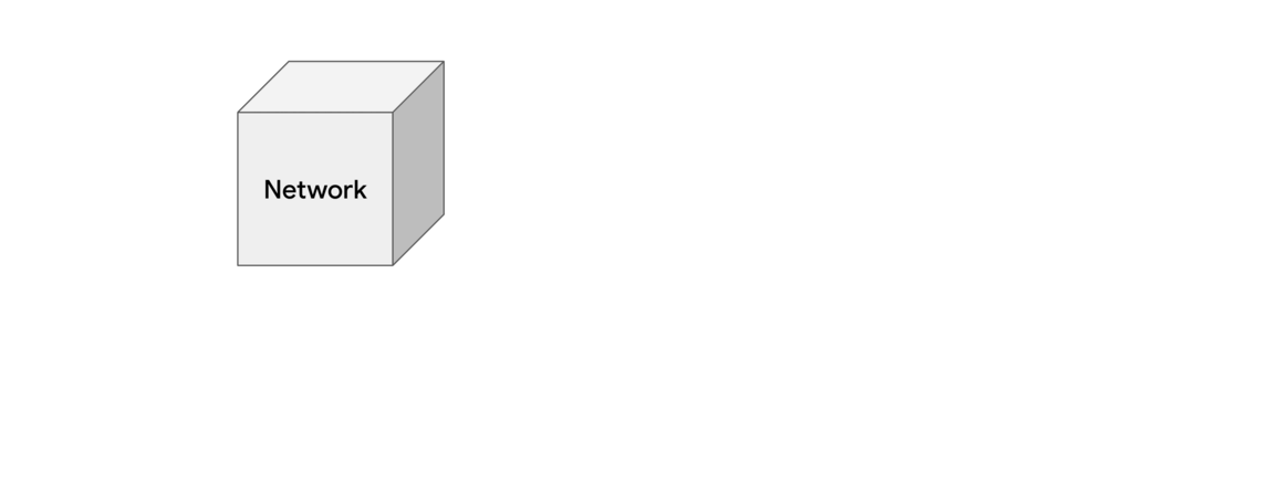
A common approach to code completion is to train transformer models, which use a self-attention mechanism for language understanding, to enable code understanding and completion predictions. We treat code similar to language, represented with sub-word tokens and a SentencePiece vocabulary, and use encoder-decoder transformer models running on TPUs to make completion predictions. The input is the code that is surrounding the cursor (~1000-2000 tokens) and the output is a set of suggestions to complete the current or multiple lines. Sequences are generated with a beam search (or tree exploration) on the decoder.

During training on Google’s monorepo, we mask out the remainder of a line and some follow-up lines, to mimic code that is being actively developed. We train a single model on eight languages (C++, Java, Python, Go, Typescript, Proto, Kotlin, and Dart) and observe improved or equal performance across all languages, removing the need for dedicated models. Moreover, we find that a model size of ~0.5B parameters gives a good tradeoff for high prediction accuracy with low latency and resource cost. The model strongly benefits from the quality of the monorepo, which is enforced by guidelines and reviews. For multi-line suggestions, we iteratively apply the single-line model with learned thresholds for deciding whether to start predicting completions for the following line.

Encoder-decoder transformer models are used to predict the remainder of the line or lines of code.

Re-rank Single Token Suggestions with ML
While a user is typing in the IDE, code completions are interactively requested from the ML model and the SE simultaneously in the backend. The SE typically only predicts a single token. The ML models we use predict multiple tokens until the end of the line, but we only consider the first token to match predictions from the SE. We identify the top three ML suggestions that are also contained in the SE suggestions and boost their rank to the top. The re-ranked results are then shown as suggestions for the user in the IDE.

In practice, our SEs are running in the cloud, providing language services (e.g., semantic completion, diagnostics, etc.) with which developers are familiar, and so we collocated the SEs to run on the same locations as the TPUs performing ML inference. The SEs are based on an internal library that offers compiler-like features with low latencies. Due to the design setup, where requests are done in parallel and ML is typically faster to serve (~40 ms median), we do not add any latency to completions. We observe a significant quality improvement in real usage. For 28% of accepted completions, the rank of the completion is higher due to boosting, and in 0.4% of cases it is worse. Additionally, we find that users type >10% fewer characters before accepting a completion suggestion.

Check Single / Multi-line ML Completions for Semantic Correctness
At inference time, ML models are typically unaware of code outside of their input window, and code seen during training might miss recent additions needed for completions in actively changing repositories. This leads to a common drawback of ML-powered code completion whereby the model may suggest code that looks correct, but doesn’t compile. Based on internal user experience research, this issue can lead to the erosion of user trust over time while reducing productivity gains.

We use SEs to perform fast semantic correctness checks within a given latency budget (<100ms for end-to-end completion) and use cached abstract syntax trees to enable a “full” structural understanding. Typical semantic checks include reference resolution (i.e., does this object exist), method invocation checks (e.g., confirming the method was called with a correct number of parameters), and assignability checks (to confirm the type is as expected).

For example, for the coding language Go, ~8% of suggestions contain compilation errors before semantic checks. However, the application of semantic checks filtered out 80% of uncompilable suggestions. The acceptance rate for single-line completions improved by 1.9x over the first six weeks of incorporating the feature, presumably due to increased user trust. As a comparison, for languages where we did not add semantic checking, we only saw a 1.3x increase in acceptance.

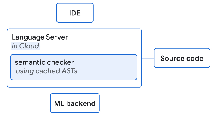
Language servers with access to source code and the ML backend are collocated on the cloud. They both perform semantic checking of ML completion suggestions.

Results
With 10k+ Google-internal developers using the completion setup in their IDE, we measured a user acceptance rate of 25-34%. We determined that the transformer-based hybrid semantic ML code completion completes >3% of code, while reducing the coding iteration time for Googlers by 6% (at a 90% confidence level). The size of the shift corresponds to typical effects observed for transformational features (e.g., key framework) that typically affect only a subpopulation, whereas ML has the potential to generalize for most major languages and engineers.

Fraction of all code added by ML 2.6%
Reduction in coding iteration duration 6%
Reduction in number of context switches 7%
Acceptance rate (for suggestions visible for >750ms) 25%
Average characters per accept 21
Key metrics for single-line code completion measured in production for 10k+ Google-internal developers using it in their daily development across eight languages.
Fraction of all code added by ML (with >1 line in suggestion) 0.6%
Average characters per accept 73
Acceptance rate (for suggestions visible for >750ms) 34%
Key metrics for multi-line code completion measured in production for 5k+ Google-internal developers using it in their daily development across eight languages.

Providing Long Completions while Exploring APIs
We also tightly integrated the semantic completion with full line completion. When the dropdown with semantic single token completions appears, we display inline the single-line completions returned from the ML model. The latter represent a continuation of the item that is the focus of the dropdown. For example, if a user looks at possible methods of an API, the inline full line completions show the full method invocation also containing all parameters of the invocation.

Integrated full line completions by ML continuing the semantic dropdown completion that is in focus.
Suggestions of multiple line completions by ML.

Conclusion and Future Work
We demonstrate how the combination of rule-based semantic engines and large language models can be used to significantly improve developer productivity with better code completion. As a next step, we want to utilize SEs further, by providing extra information to ML models at inference time. One example can be for long predictions to go back and forth between the ML and the SE, where the SE iteratively checks correctness and offers all possible continuations to the ML model. When adding new features powered by ML, we want to be mindful to go beyond just “smart” results, but ensure a positive impact on productivity.

Acknowledgements
This research is the outcome of a two-year collaboration between Google Core and Google Research, Brain Team. Special thanks to Marc Rasi, Yurun Shen, Vlad Pchelin, Charles Sutton, Varun Godbole, Jacob Austin, Danny Tarlow, Benjamin Lee, Satish Chandra, Ksenia Korovina, Stanislav Pyatykh, Cristopher Claeys, Petros Maniatis, Evgeny Gryaznov, Pavel Sychev, Chris Gorgolewski, Kristof Molnar, Alberto Elizondo, Ambar Murillo, Dominik Schulz, David Tattersall, Rishabh Singh, Manzil Zaheer, Ted Ying, Juanjo Carin, Alexander Froemmgen and Marcus Revaj for their contributions.


Source: Google AI Blog


Minerva: Solving Quantitative Reasoning Problems with Language Models

Language models have demonstrated remarkable performance on a variety of natural language tasks — indeed, a general lesson from many works, including BERT, GPT-3, Gopher, and PaLM, has been that neural networks trained on diverse data at large scale in an unsupervised way can perform well on a variety of tasks.

Quantitative reasoning is one area in which language models still fall far short of human-level performance. Solving mathematical and scientific questions requires a combination of skills, including correctly parsing a question with natural language and mathematical notation, recalling relevant formulas and constants, and generating step-by-step solutions involving numerical calculations and symbolic manipulation. Due to these challenges, it is often believed that solving quantitative reasoning problems using machine learning will require significant advancements in model architecture and training techniques, granting models access to external tools such as Python interpreters, or possibly a more profound paradigm shift.

In “Solving Quantitative Reasoning Problems With Language Models” (to be released soon on the arXiv), we present Minerva, a language model capable of solving mathematical and scientific questions using step-by-step reasoning. We show that by focusing on collecting training data that is relevant for quantitative reasoning problems, training models at scale, and employing best-in-class inference techniques, we achieve significant performance gains on a variety of difficult quantitative reasoning tasks. Minerva solves such problems by generating solutions that include numerical calculations and symbolic manipulation without relying on external tools such as a calculator. The model parses and answers mathematical questions using a mix of natural language and mathematical notation. Minerva combines several techniques, including few-shot prompting, chain of thought or scratchpad prompting, and majority voting, to achieve state-of-the-art performance on STEM reasoning tasks. You can explore Minerva’s output with our interactive sample explorer!

Solving a multi-step problem: A question from the MATH dataset and Minerva’s solution. The model writes down a line equation, simplifies it, substitutes a variable, and solves for y.

A Model Built for Multi-step Quantitative Reasoning
To promote quantitative reasoning, Minerva builds on the Pathways Language Model (PaLM), with further training on a 118GB dataset of scientific papers from the arXiv preprint server and web pages that contain mathematical expressions using LaTeX, MathJax, or other mathematical typesetting formats. Standard text cleaning procedures often remove symbols and formatting that are essential to the semantic meaning of mathematical expressions. By maintaining this information in the training data, the model learns to converse using standard mathematical notation.

Example questions from the Joint Entrance Examination Main Math 2020 exam taken each year by almost 2M Indian high-school students intended to study engineering and similar fields (left), and the National Math Exam in Poland (May 2022) taken by approximately 270K high-school students every year (right).
A dataset for quantitative reasoning: Careful data processing preserves mathematical information, allowing the model to learn mathematics at a higher level.

Minerva also incorporates recent prompting and evaluation techniques to better solve mathematical questions. These include chain of thought or scratchpad prompting — where Minerva is prompted with several step-by-step solutions to existing questions before being presented with a new question — and majority voting. Like most language models, Minerva assigns probabilities to different possible outputs. When answering a question, rather than taking the single solution Minerva scores as most likely, multiple solutions are generated by sampling stochastically from all possible outputs. These solutions are different (e.g., the steps are not identical), but often arrive at the same final answer. Minerva uses majority voting on these sampled solutions, taking the most common result as the conclusive final answer.

Majority voting: Minerva generates multiple solutions to each question and chooses the most common answer as the solution, improving performance significantly.

Evaluation on STEM Benchmarks
To test Minerva’s quantitative reasoning abilities we evaluated the model on STEM benchmarks ranging in difficulty from grade school level problems to graduate level coursework.

  • MATH: High school math competition level problems
  • MMLU-STEM: A subset of the Massive Multitask Language Understanding benchmark focused on STEM, covering topics such as engineering, chemistry, math, and physics at high school and college level.
  • GSM8k: Grade school level math problems involving basic arithmetic operations that should all be solvable by a talented middle school student.

We also evaluated Minerva on OCWCourses, a collection of college and graduate level problems covering a variety of STEM topics such as solid state chemistry, astronomy, differential equations, and special relativity that we collected from MIT OpenCourseWare.

In all cases, Minerva obtains state-of-the-art results, sometimes by a wide margin.

Evaluation results on MATH and MMLU-STEM, which include high school and college level questions covering a range of STEM topics.
Model   MATH     MMLU-STEM     OCWCourses     GSM8k  
Minerva 50.3% 75% 30.8% 78.5%
Published state of the art    6.9% 55% - 74.4%
Minerva 540B significantly improves state-of-the-art performance on STEM evaluation datasets.

What Minerva Gets Wrong
Minerva still makes its fair share of mistakes. To better identify areas where the model can be improved, we analyzed a sample of questions the model gets wrong, and found that most mistakes are easily interpretable. About half are calculation mistakes, and the other half are reasoning errors, where the solution steps do not follow a logical chain of thought.

It is also possible for the model to arrive at a correct final answer but with faulty reasoning. We call such cases “false positives”, as they erroneously count toward a model’s overall performance score. In our analysis, we find that the rate of false positives is relatively low (Minerva 62B produces less than 8% false positives on MATH).

Below are a couple of example mistakes the model makes.

Calculation mistake: The model incorrectly cancels the square root on both sides of the equation.
Reasoning mistake: The model computes the number of free throws at the fourth practice, but then uses this number as the final answer for the first practice.

Limitations
Our approach to quantitative reasoning is not grounded in formal mathematics. Minerva parses questions and generates answers using a mix of natural language and LaTeX mathematical expressions, with no explicit underlying mathematical structure. This approach has an important limitation, in that the model’s answers cannot be automatically verified. Even when the final answer is known and can be verified, the model can arrive at a correct final answer using incorrect reasoning steps, which cannot be automatically detected. This limitation is not present in formal methods for theorem proving (e.g., see Coq, Isabelle, HOL, Lean, Metamath, and Mizar). On the other hand, an advantage of the informal approach is that it can be applied to a highly diverse set of problems which may not lend themselves to formalization.

Future Directions
While machine learning models have become impressive tools in many scientific disciplines, they are often narrowly scoped to solve specific tasks. We hope that general models capable of solving quantitative reasoning problems will help push the frontiers of science and education. Models capable of quantitative reasoning have many potential applications, including serving as useful aids for researchers, and enabling new learning opportunities for students. We present Minerva as a small step in this direction. To see more samples from Minerva, such as the one below, please visit the interactive sample explorer!

Solving a problem using calculus and trigonoometry: A question from the MATH dataset asking for the speed of a particle in circular motion. Minerva finds a correct step-by-step solution. In the process, Minerva computes a time derivative and applies a trigonometric identity.

Acknowledgements
Minerva was a collaborative effort that spanned multiple teams in Google Research. We would like to thank our coauthors Aitor Lewkowycz, Ambrose Slone, Anders Andreassen, Behnam Neyshabur, Cem Anil, David Dohan, Henryk Michalewski, Imanol Schlag, Theo Gutman-Solo, Vedant Misra, Vinay Ramasesh, and Yuhuai Wu, as well as our collaborators Erik Zelikman and Yasaman Razeghi. Minerva builds upon the work of many others at Google, and we would like to thank the PaLM team, the T5X team, the Flaxformer team, and the JAX team for their efforts. We thank Tom Small for designing the animation in this post. We would also like to especially thank Vedant Misra for developing the Minerva sample explorer.

Source: Google AI Blog


LIMoE: Learning Multiple Modalities with One Sparse Mixture of Experts Model

Sparse models stand out among the most promising approaches for the future of deep learning. Instead of every part of a model processing every input (“dense” modeling), sparse models employing conditional computation learn to route individual inputs to different “experts” in a potentially huge network. This has many benefits. First, model size can increase while keeping computational cost constant — an effective and environmentally friendlier way to scale models, which is often key to high performance. Sparsity also naturally compartmentalizes neural networks. Dense models that learn many different tasks simultaneously (multitask) or sequentially (continual learning) often suffer negative interference, where too much task variety means it is better to just train one model per task, or catastrophic forgetting, where the model becomes worse at earlier tasks as new ones are added. Sparse models help avoid both these phenomena — by not applying the whole model to all inputs, “experts” in the model can specialize on different tasks or data types while still taking advantage of shared parts of the model.

Research on sparsity has long been pursued at Google Research. Pathways summarizes the research vision of building one single large model that diligently handles thousands of tasks and numerous data modalities. So far there has been considerable progress in sparse unimodal models for language (Switch, Task-MoE, GLaM) and computer vision (Vision MoE). Today, we take another important step towards the Pathways vision by studying large sparse models that simultaneously handle images and text with modality-agnostic routing. A relevant approach is multimodal contrastive learning, which requires a solid understanding of both images and text in order to align pictures with their correct text description. The strongest models that tackle this task to date rely on independent networks for each modality (a “two-tower” approach).

In “Multimodal Contrastive Learning with LIMoE: the Language Image Mixture of Experts”, we present the first large-scale multimodal architecture using a sparse mixture of experts. It simultaneously processes both images and text, but uses sparsely activated experts that naturally specialize. On zero-shot image classification, LIMoE outperforms both comparable dense multimodal models and two-tower approaches. The largest LIMoE achieves 84.1% zero-shot ImageNet accuracy, comparable to more expensive state-of-the-art models. Sparsity enables LIMoE to scale up gracefully and learn to handle very different inputs, addressing the tension between being a jack-of-all-trades generalist and a master-of-one specialist.

The LIMoE architecture contains many “experts” and routers decide which tokens (parts of an image or sentence) go to which experts. After being processed by expert layers (gray) and shared dense layers (brown), a final output layer computes a single vector representation for either an image or a text.

Sparse Mixture of Expert Models
Transformers represent data as a sequence of vectors (or tokens). Though originally developed for text, they can be applied to most things that are representable as a sequence of tokens, e.g., images, videos, and audio. Recent large-scale MoE models add expert layers to the Transformer architecture (e.g., gShard and ST-MoE in natural language processing, and Vision MoE for vision tasks).

A standard Transformer consists of many “blocks”, each containing various different layers. One of these layers is a feed-forward network (FFN). For LIMoE and the works cited above, this single FFN is replaced by an expert layer that contains many parallel FFNs, each of which is an expert. Given a sequence of tokens to process, a simple router learns to predict which experts should handle which tokens. Only a small number of experts are activated per token, meaning although the model capacity is significantly increased by virtue of having so many experts, the actual computational cost is controlled by using them sparsely. If only one expert is activated, the model's cost is roughly equivalent to the standard Transformer model.

LIMoE does precisely that, activating one expert per example, thereby matching the computational cost of the dense baselines. What’s different is that the LIMoE router might see tokens of either image or text data.

A unique failure mode of MoE models occurs when they try to send all tokens to the same expert. Typically this is addressed with auxiliary losses, extra training objectives that encourage balanced expert usage. We found that dealing with multiple modalities interacted with sparsity to cause new failure modes that existing auxiliary losses could not address. To overcome this, we developed new auxiliary losses (more details in the paper) and used routing prioritization (BPR) during training, two innovations that resulted in stable and high performance multimodal models.

The new auxiliary losses (LIMoE aux) and routing prioritization (BPR) stabilized and improved overall performance (left) and increased the success rate of routing behavior (middle and right). A low success rate means the router does not use all the experts available and drops many tokens due to individual expert capacity being reached, which usually indicates the sparse model is not learning well. The combination introduced for LIMoE ensures high routing success rates for both images and text and consequently leads to significantly better performance.

Contrastive Learning with LIMoE
In multimodal contrastive learning, models are trained on paired image-text data (e.g., a photo and its caption). Typically, an image model extracts a representation of images, and a different text model extracts a representation of text. The contrastive learning objective encourages the image and text representations to be close for the same image-text pair and far away for content from different pairs. Such models with aligned representations can be adapted to new tasks without extra training data (“zero-shot”), e.g., an image will be classified as a dog if its representation is closer to the representation of the word “dog” than the word “cat”. This idea scales to thousands of classes and is referred to as zero-shot image classification.

CLIP and ALIGN (both two-tower models) scaled this process to achieve 76.2% and 76.4% zero-shot classification accuracy on the popular ImageNet dataset. We study one-tower models which compute both image and text representations. We find this reduces performance for dense models, likely due to negative interference or insufficient capacity. However, a compute-matched LIMoE not only improves over the one-tower dense model, but also outperforms two-tower dense models. We trained a series of models in a comparable training regimen to CLIP. Our dense L/16 model achieves 73.5% zero-shot accuracy, whereas LIMoE-L/16 gets to 78.6%, even outperforming CLIP’s more expensive, two-tower L/14 model (76.2%). As shown below, LIMoE’s use of sparsity provides a remarkable performance boost over dense models with equivalent cost.

For a given compute cost (x-axis), LIMoE models (circles, solid line) are significantly better than their dense baselines (triangles, dashed line). The architecture indicates the size of the underlying transformer, increasing from left (S/32) to right (L/16). Following standard convention, S (small), B (base), and L (large) refer to model scale. The number refers to the patch size, where smaller patches imply a larger architecture.

LiT and BASIC pushed zero-shot accuracy for dense two-tower models to 84.5% and 85.6% respectively. In addition to scaling, these approaches made use of specialized pre-training methods, repurposing image models that were already of exceptionally high quality. LIMoE-H/14 does not benefit from any pre-training or modality-specific components, but still achieved a comparable 84.1% zero-shot accuracy training from scratch. The scale of these models is also interesting to compare: LiT and BASIC are 2.1B and 3B parameter models. LIMoE-H/14 has 5.6B parameters in total, but via sparsity it only applies 675M parameters per token making it significantly more lightweight.

Data seen during training
Model   Pre-training     Image-text     Total      Parameters per token     ImageNet accuracy  
CLIP - 12.8B 12.8B ~200M 76.2%
ALIGN - 19.8B 19.8B ~410M 76.4%
LiT 25.8B 18.2B 44.0B 1.1B 84.5%
BASIC 19.7B 32.8B 52.5B 1.5B 85.6%
LIMoE H/14    - 23.3B 23.3B 675M 84.1%

Understanding LIMoE’s Behavior
LIMoE was motivated by the intuition that sparse conditional computation enables a generalist multimodal model to still develop the specialization needed to excel at understanding each modality. We analyzed LIMoE’s expert layers and uncovered a few interesting phenomena.

First, we see the emergence of modality-specialized experts. In our training setup there are many more image tokens than text tokens, so all experts tend to process at least some images, but some experts process either mostly images, mostly text, or both.

Distributions for an eight expert LIMoE; percentages indicate the amount of image tokens processed by the expert. There are one or two experts clearly specialized on text (shown by the mostly blue experts), usually two to four image specialists (mostly red), and the remainder are somewhere in the middle.

There are also some clear qualitative patterns among the image experts — e.g., in most LIMoE models, there is an expert that processes all image patches that contain text. In the example below, one expert processes fauna and greenery, and another processes human hands.

LIMoE chooses an expert for each token. Here we show which image tokens go to which experts on one of the layers of LIMoE-H/14. Despite not being trained to do so, we observe the emergence of semantic experts that specialize in specific topics such as plants or wheels.

Moving Forward
Multimodal models that handle many tasks are a promising route forward, and there are two key ingredients for success: scale, and the ability to avoid interference between distinct tasks and modalities while taking advantage of synergies. Sparse conditional computation is an excellent way of doing both. It enables performant and efficient generalist models that also have the capacity and flexibility for the specialization necessary to excel at individual tasks, as demonstrated by LIMoE’s solid performance with less compute.

Acknowledgements
We thank our co-authors on this work: Joan Puigcerver, Rodolphe Jenatton and Neil Houlsby. We also thank Andreas Steiner, Xiao Wang and Xiaohua Zhai, who led early explorations into dense single-tower models for contrastive multimodal learning, and also were instrumental in providing data access. We enjoyed useful discussions with André Susano Pinto, Maxim Neumann, Barret Zoph, Liam Fedus, Wei Han and Josip Djolonga. Finally, we would also like to thank and acknowledge Tom Small for the awesome animated figure used in this post.

Source: Google AI Blog


Pix2Seq: A New Language Interface for Object Detection

Object detection is a long-standing computer vision task that attempts to recognize and localize all objects of interest in an image. The complexity arises when trying to identify or localize all object instances while also avoiding duplication. Existing approaches, like Faster R-CNN and DETR, are carefully designed and highly customized in the choice of architecture and loss function. This specialization of existing systems has created two major barriers: (1) it adds complexity in tuning and training the different parts of the system (e.g., region proposal network, graph matching with GIOU loss, etc.), and (2), it can reduce the ability of a model to generalize, necessitating a redesign of the model for application to other tasks.

In “Pix2Seq: A Language Modeling Framework for Object Detection”, published at ICLR 2022, we present a simple and generic method that tackles object detection from a completely different perspective. Unlike existing approaches that are task-specific, we cast object detection as a language modeling task conditioned on the observed pixel inputs. We demonstrate that Pix2Seq achieves competitive results on the large-scale object detection COCO dataset compared to existing highly-specialized and well-optimized detection algorithms, and its performance can be further improved by pre-training the model on a larger object detection dataset. To encourage further research in this direction, we are also excited to release to the broader research community Pix2Seq’s code and pre-trained models along with an interactive demo.

Pix2Seq Overview
Our approach is based on the intuition that if a neural network knows where and what the objects in an image are, one could simply teach it how to read them out. By learning to “describe” objects, the model can learn to ground the descriptions on pixel observations, leading to useful object representations. Given an image, the Pix2Seq model outputs a sequence of object descriptions, where each object is described using five discrete tokens: the coordinates of the bounding box’s corners [ymin, xmin, ymax, xmax] and a class label.

Pix2Seq framework for object detection. The neural network perceives an image, and generates a sequence of tokens for each object, which correspond to bounding boxes and class labels.

With Pix2Seq, we propose a quantization and serialization scheme that converts bounding boxes and class labels into sequences of discrete tokens (similar to captions), and leverage an encoder-decoder architecture to perceive pixel inputs and generate the sequence of object descriptions. The training objective function is simply the maximum likelihood of tokens conditioned on pixel inputs and the preceding tokens.

Sequence Construction from Object Descriptions
In commonly used object detection datasets, images have variable numbers of objects, represented as sets of bounding boxes and class labels. In Pix2Seq, a single object, defined by a bounding box and class label, is represented as [ymin, xmin, ymax, xmax, class]. However, typical language models are designed to process discrete tokens (or integers) and are unable to comprehend continuous numbers. So, instead of representing image coordinates as continuous numbers, we normalize the coordinates between 0 and 1 and quantize them into one of a few hundred or thousand discrete bins. The coordinates are then converted into discrete tokens as are the object descriptions, similar to image captions, which in turn can then be interpreted by the language model. The quantization process is achieved by multiplying the normalized coordinate (e.g., ymin) by the number of bins minus one, and rounding it to the nearest integer (the detailed process can be found in our paper).

Quantization of the coordinates of the bounding boxes with different numbers of bins on a 480 × 640 image. With a small number of bins/tokens, such as 500 bins (∼1 pixel/bin), it achieves high precision even for small objects.

After quantization, the object annotations provided with each training image are ordered into a sequence of discrete tokens (shown below). Since the order of the objects does not matter for the detection task per se, we randomize the order of objects each time an image is shown during training. We also append an End of Sequence (EOS) token at the end as​​ different images often have different numbers of objects, and hence sequence lengths.

The bounding boxes and class labels for objects detected in the image on the left are represented in the sequences shown on the right. A random object ordering strategy is used in our work but other approaches to ordering could also be used.

The Model Architecture, Objective Function, and Inference
We treat the sequences that we constructed from object descriptions as a “dialect” and address the problem via a powerful and general language model with an image encoder and autoregressive language encoder. Similar to language modeling, Pix2Seq is trained to predict tokens, given an image and preceding tokens, with a maximum likelihood loss. At inference time, we sample tokens from model likelihood. The sampled sequence ends when the EOS token is generated. Once the sequence is generated, we split it into chunks of 5 tokens for extracting and de-quantizing the object descriptions (i.e., obtaining the predicted bounding boxes and class labels). It is worth noting that both the architecture and loss function are task-agnostic in that they don’t assume prior knowledge about object detection (e.g., bounding boxes). We describe how we can incorporate task-specific prior knowledge with a sequence augmentation technique in our paper.

Results
Despite its simplicity, Pix2Seq achieves impressive empirical performance on benchmark datasets. Specifically, we compare our method with well established baselines, Faster R-CNN and DETR, on the widely used COCO dataset and demonstrate that it achieves competitive average precision (AP) results.

Pix2Seq achieves competitive AP results compared to existing systems that require specialization during model design, while being significantly simpler. The best performing Pix2Seq model achieved an AP score of 45.

Since our approach incorporates minimal inductive bias or prior knowledge of the object detection task into the model design, we further explore how pre-training the model using the large-scale object detection COCO dataset can impact its performance. Our results indicate that this training strategy (along with using bigger models) can further boost performance.

The average precision of the Pix2Seq model with pre-training followed by fine-tuning. The best performing Pix2Seq model without pre-training achieved an AP score of 45. When the model is pre-trained, we see an 11% improvement with an AP score of 50.

Pix2Seq can detect objects in densely populated and complex scenes, such as those shown below.

Example complex and densely populated scenes labeled by a trained Pix2Seq model. Try it out here.

Conclusion and Future Work
With Pix2Seq, we cast object detection as a language modeling task conditioned on pixel inputs for which the model architecture and loss function are generic, and have not been engineered specifically for the detection task. One can, therefore, readily extend this framework to different domains or applications, where the output of the system can be represented by a relatively concise sequence of discrete tokens (e.g., keypoint detection, image captioning, visual question answering), or incorporate it into a perceptual system supporting general intelligence, for which it provides a language interface to a wide range of vision and language tasks. We also hope that the release of our Pix2Seq’s code, pre-trained models and interactive demo will inspire further research in this direction.

Acknowledgements
This post reflects the combined work with our co-authors: Saurabh Saxena, Lala Li, Geoffrey Hinton. We would also like to thank Tom Small for the visualization of the Pix2Seq illustration figure.

Source: Google AI Blog


Learning to Prompt for Continual Learning

Supervised learning is a common approach to machine learning (ML) in which the model is trained using data that is labeled appropriately for the task at hand. Ordinary supervised learning trains on independent and identically distributed (IID) data, where all training examples are sampled from a fixed set of classes, and the model has access to these examples throughout the entire training phase. In contrast, continual learning tackles the problem of training a single model on changing data distributions where different classification tasks are presented sequentially. This is particularly important, for example, to enable autonomous agents to process and interpret continuous streams of information in real-world scenarios.

To illustrate the difference between supervised and continual learning, consider two tasks: (1) classify cats vs. dogs and (2) classify pandas vs. koalas. In supervised learning, which uses IID, the model is given training data from both tasks and treats it as a single 4-class classification problem. However, in continual learning, these two tasks arrive sequentially, and the model only has access to the training data of the current task. As a result, such models tend to suffer from performance degradation on the previous tasks, a phenomenon called catastrophic forgetting.

Mainstream solutions try to address catastrophic forgetting by buffering past data in a “rehearsal buffer” and mixing it with current data to train the model. However, the performance of these solutions depends heavily on the size of the buffer and, in some cases, may not be possible at all due to data privacy concerns. Another branch of work designs task-specific components to avoid interference between tasks. But these methods often assume that the task at test time is known, which is not always true, and they require a large number of parameters. The limitations of these approaches raise critical questions for continual learning: (1) Is it possible to have a more effective and compact memory system that goes beyond buffering past data? (2) Can one automatically select relevant knowledge components for an arbitrary sample without knowing its task identity?

In “Learning to Prompt for Continual Learning”, presented at CVPR2022, we attempt to answer these questions. Drawing inspiration from prompting techniques in natural language processing, we propose a novel continual learning framework called Learning to Prompt (L2P). Instead of continually re-learning all the model weights for each sequential task, we instead provide learnable task-relevant “instructions'' (i.e., prompts) to guide pre-trained backbone models through sequential training via a pool of learnable prompt parameters. L2P is applicable to various challenging continual learning settings and outperforms previous state-of-the-art methods consistently on all benchmarks. It achieves competitive results against rehearsal-based methods while also being more memory efficient. Most importantly, L2P is the first to introduce the idea of prompting in the field of continual learning.

Compared with typical methods that adapt entire or partial model weights to tasks sequentially using a rehearsal buffer, L2P uses a single frozen backbone model and learns a prompt pool to conditionally instruct the model. “Model 0” indicates that the backbone model is fixed at the beginning.

Prompt Pool and Instance-Wise Query
Given a pre-trained Transformer model, “prompt-based learning” modifies the original input using a fixed template. Imagine a sentiment analysis task is given the input “I like this cat”. A prompt-based method will transform the input to “I like this cat. It looks X”, where the “X” is an empty slot to be predicted (e.g., “nice”, “cute”, etc.) and “It looks X” is the so-called prompt. By adding prompts to the input, one can condition the pre-trained models to solve many downstream tasks. While designing fixed prompts requires prior knowledge along with trial and error, prompt tuning prepends a set of learnable prompts to the input embedding to instruct the pre-trained backbone to learn a single downstream task, under the transfer learning setting.

In the continual learning scenario, L2P maintains a learnable prompt pool, where prompts can be flexibly grouped as subsets to work jointly. Specifically, each prompt is associated with a key that is learned by reducing the cosine similarity loss between matched input query features. These keys are then utilized by a query function to dynamically look up a subset of task-relevant prompts based on the input features. At test time, inputs are mapped by the query function to the top-N closest keys in the prompt pool, and the associated prompt embeddings are then fed to the rest of the model to generate the output prediction. At training, we optimize the prompt pool and the classification head via the cross-entropy loss.

Illustration of L2P at test time. First, L2P selects a subset of prompts from a key-value paired prompt pool based on our proposed instance-wise query mechanism. Then, L2P prepends the selected prompts to the input tokens. Finally, L2P feeds the extended tokens to the model for prediction.

Intuitively, similar input examples tend to choose similar sets of prompts and vice versa. Thus, prompts that are frequently shared encode more generic knowledge while other prompts encode more task-specific knowledge. Moreover, prompts store high-level instructions and keep lower-level pre-trained representations frozen, thus catastrophic forgetting is mitigated even without the necessity of a rehearsal buffer. The instance-wise query mechanism removes the necessity of knowing the task identity or boundaries, enabling this approach to address the under-investigated challenge of task-agnostic continual learning.

Effectiveness of L2P
We evaluate the effectiveness of L2P in different baseline methods using an ImageNet pre-trained Vision Transformer (ViT) on representative benchmarks. The naïve baseline, called Sequential in the graphs below, refers to training a single model sequentially on all tasks. The EWC model adds a regularization term to mitigate forgetting and the Rehearsal model saves past examples to a buffer for mixed training with current data. To measure the overall continual learning performance, we measure both the accuracy and the average difference between the best accuracy achieved during training and the final accuracy for all tasks (except the last task), which we call forgetting. We find that L2P outperforms the Sequential and EWC methods significantly in both metrics. Notably, L2P even surpasses the Rehearsal approach, which uses an additional buffer to save past data. Because the L2P approach is orthogonal to Rehearsal, its performance could be further improved if it, too, used a rehearsal buffer.

L2P outperforms baseline methods in both accuracy (top) and forgetting (bottom). Accuracy refers to the average accuracy for all tasks and forgetting is defined as the average difference between the best accuracy achieved during training and the final accuracy for all tasks (except the last task).

We also visualize the prompt selection result from our instance-wise query strategy on two different benchmarks, where one has similar tasks and the other has varied tasks. The results indicate that L2P promotes more knowledge sharing between similar tasks by having more shared prompts, and less knowledge sharing between varied tasks by having more task-specific prompts.

Prompt selection histograms for benchmarks of similar tasks (left) and varied tasks (right). The left benchmark has higher intra-task similarity, thus sharing prompts between tasks results in good performance, while the right benchmark favors more task-specific prompts.

Conclusion
In this work, we present L2P to address key challenges in continual learning from a new perspective. L2P does not require a rehearsal buffer or known task identity at test time to achieve high performance. Further, it can handle various complex continual learning scenarios, including the challenging task-agnostic setting. Because large-scale pre-trained models are widely used in the machine learning community for their robust performance on real-world problems, we believe that L2P opens a new learning paradigm towards practical continual learning applications.

Acknowledgements
We gratefully acknowledge the contributions of other co-authors, including Chen-Yu Lee, Han Zhang, Ruoxi Sun, Xiaoqi Ren, Guolong Su, Vincent Perot, Jennifer Dy, Tomas Pfister. We would also like to thank Chun-Liang Li, Jeremy Martin Kubica, Sayna Ebrahimi, Stratis Ioannidis, Nan Hua, and Emmanouil Koukoumidis, for their valuable discussions and feedback, and Tom Small for figure creation.

Source: Google AI Blog


Reproducibility in Deep Learning and Smooth Activations

Ever queried a recommender system and found that the same search only a few moments later or on a different device yields very different results? This is not uncommon and can be frustrating if a person is looking for something specific. As a designer of such a system, it is also not uncommon for the metrics measured to change from design and testing to deployment, bringing into question the utility of the experimental testing phase. Some level of such irreproducibility can be expected as the world changes and new models are deployed. However, this also happens regularly as requests hit duplicates of the same model or models are being refreshed.

Lack of replicability, where researchers are unable to reproduce published results with a given model, has been identified as a challenge in the field of machine learning (ML). Irreproducibility is a related but more elusive problem, where multiple instances of a given model are trained on the same data under identical training conditions, but yield different results. Only recently has irreproducibility been identified as a difficult problem, but due to its complexity, theoretical studies to understand this problem are extremely rare.

In practice, deep network models are trained in highly parallelized and distributed environments. Nondeterminism in training from random initialization, parallelism, distributed training, data shuffling, quantization errors, hardware types, and more, combined with objectives with multiple local optima contribute to the problem of irreproducibility. Some of these factors, such as initialization, can be controlled, but it is impractical to control others. Optimization trajectories can diverge early in training by following training examples in the order seen, leading to very different models. Several recently published solutions [1, 2, 3] based on advanced combinations of ensembling, self-ensembling, and distillation can mitigate the problem, but usually at the cost of accuracy and increased complexity, maintenance and improvement costs.

In “Real World Large Scale Recommendation Systems Reproducibility and Smooth Activations”, we consider a different practical solution to this problem that does not incur the costs of other solutions, while still improving reproducibility and yielding higher model accuracy. We discover that the Rectified Linear Unit (ReLU), which is very popular as the nonlinearity function (i.e., activation function) used to transform values in neural networks, exacerbates the irreproducibility problem. On the other hand, we demonstrate that smooth activation functions, which have derivatives that are continuous for the whole domain, unlike those of ReLU, are able to substantially reduce irreproducibility levels. We then propose the Smooth reLU (SmeLU) activation function, which gives comparable reproducibility and accuracy benefits to other smooth activations but is much simpler.

The ReLU function (left) as function of the input signal, and its gradient (right) as function of the input.

Smooth Activations
An ML model attempts to learn the best model parameters that fit the training data by minimizing a loss, which can be imagined as a landscape with peaks and valleys, where the lowest point attains an optimal solution. For deep models, the landscape may consist of many such peaks and valleys. The activation function used by the model governs the shape of this landscape and how the model navigates it.

ReLU, which is not a smooth function, imposes an objective whose landscape is partitioned into many regions with multiple local minima, each providing different model predictions. With this landscape, the order in which updates are applied is a dominant factor in determining the optimization trajectory, providing a recipe for irreproducibility. Because of its non-continuous gradient, functions expressed by a ReLU network will contain sudden jumps in the gradient, which can occur internally in different layers of the deep network, affecting updates of different internal units, and are likely strong contributors to irreproducibility.

Suppose a sequence of model updates attempts to push the activation of some unit down from a positive value. The gradient of the ReLU function is 1 for positive unit values, so with every update it pushes the unit to become smaller and smaller (to the left in the panel above). At the point the activation of this unit crosses the threshold from a positive value to a negative one, the gradient suddenly changes from magnitude 1 to magnitude 0. Training attempts to keep moving the unit leftwards, but due to the 0 gradient, the unit cannot move further in that direction. Therefore, the model must resort to updating other units that can move.

We find that networks with smooth activations (e.g., GELU, Swish and Softplus) can be substantially more reproducible. They may exhibit a similar objective landscape, but with fewer regions, giving a model fewer opportunities to diverge. Unlike the sudden jumps with ReLU, for a unit with decreasing activations, the gradient gradually reduces to 0, which gives other units opportunities to adjust to the changing behavior. With equal initialization, moderate shuffling of training examples, and normalization of hidden layer outputs, smooth activations are able to increase the chances of converging to the same minimum. Very aggressive data shuffling, however, loses this advantage.

The rate that a smooth activation function transitions between output levels, i.e., its “smoothness”, can be adjusted. Sufficient smoothness leads to improved accuracy and reproducibility. Too much smoothness, though, approaches linear models with a corresponding degradation of model accuracy, thus losing the advantages of using a deep network.

Smooth activations (top) and their gradients (bottom) for different smoothness parameter values β as a function of the input values. β determines the width of the transition region between 0 and 1 gradients. For Swish and Softplus, a greater β gives a narrower region, for SmeLU, a greater β gives a wider region.

Smooth reLU (SmeLU)
Activations like GELU and Swish require complex hardware implementations to support exponential and logarithmic functions. Further, GELU must be computed numerically or approximated. These properties can make deployment error-prone, expensive, or slow. GELU and Swish are not monotonic (they start by slightly decreasing and then switch to increasing), which may interfere with interpretability (or identifiability), nor do they have a full stop or a clean slope 1 region, properties that simplify implementation and may aid in reproducibility. 

The Smooth reLU (SmeLU) activation function is designed as a simple function that addresses the concerns with other smooth activations. It connects a 0 slope on the left with a slope 1 line on the right through a quadratic middle region, constraining continuous gradients at the connection points (as an asymmetric version of a Huber loss function).

SmeLU can be viewed as a convolution of ReLU with a box. It provides a cheap and simple smooth solution that is comparable in reproducibility-accuracy tradeoffs to more computationally expensive and complex smooth activations. The figure below illustrates the transition of the loss (objective) surface as we gradually transition from a non-smooth ReLU to a smoother SmeLU. A transition of width 0 is the basic ReLU function for which the loss objective has many local minima. As the transition region widens (SmeLU), the loss surface becomes smoother. If the transition is too wide, i.e., too smooth, the benefit of using a deep network wanes and we approach the linear model solution — the objective surface flattens, potentially losing the ability of the network to express much information.

Loss surfaces (as functions of a 2D input) for two sample loss functions (middle and right) as the activation function’s transition region widens, going from from ReLU to an increasingly smoother SmeLU (left). The loss surface becomes smoother with increasing the smoothness of the SmeLU function.

Performance
SmeLU has benefited multiple systems, specifically recommendation systems, increasing their reproducibility by reducing, for example, recommendation swap rates. While the use of SmeLU results in accuracy improvements over ReLU, it also replaces other costly methods to address irreproducibility, such as ensembles, which mitigate irreproducibility at the cost of accuracy. Moreover, replacing ensembles in sparse recommendation systems reduces the need for multiple lookups of model parameters that are needed to generate an inference for each of the ensemble components. This substantially improves training and inference efficiency.

To illustrate the benefits of smooth activations, we plot the relative prediction difference (PD) as a function of change in some loss for the different activations. We define relative PD as the ratio between the absolute difference in predictions of two models and their expected prediction, averaged over all evaluation examples. We have observed that in large scale systems, it is sufficient, and inexpensive, to consider only two models for very consistent results.

The figure below shows curves on the PD-accuracy loss plane. For reproducibility, being lower on the curve is better, and for accuracy, being on the left is better. Smooth activations can yield a ballpark 50% reduction in PD relative to ReLU, while still potentially resulting in improved accuracy. SmeLU yields accuracy comparable to other smooth activations, but is more reproducible (lower PD) while still outperforming ReLU in accuracy.

Relative PD as a function of percentage change in the evaluation ranking loss, which measures how accurately items are ranked in a recommendation system (higher values indicate worse accuracy), for different activations.

Conclusion and Future Work
We demonstrated the problem of irreproducibility in real world practical systems, and how it affects users as well as system and model designers. While this particular issue has been given very little attention when trying to address the lack of replicability of research results, irreproducibility can be a critical problem. We demonstrated that a simple solution of using smooth activations can substantially reduce the problem without degrading other critical metrics like model accuracy. We demonstrate a new smooth activation function, SmeLU, which has the added benefits of mathematical simplicity and ease of implementation, and can be cheap and less error prone.

Understanding reproducibility, especially in deep networks, where objectives are not convex, is an open problem. An initial theoretical framework for the simpler convex case has recently been proposed, but more research must be done to gain a better understanding of this problem which will apply to practical systems that rely on deep networks.

Acknowledgements
We would like to thank Sergey Ioffe for early discussions about SmeLU; Lorenzo Coviello and Angel Yu for help in early adoptions of SmeLU; Shiv Venkataraman for sponsorship of the work; Claire Cui for discussion and support from the very beginning; Jeremiah Willcock, Tom Jablin, and Cliff Young for substantial implementation support; Yuyan Wang, Mahesh Sathiamoorthy, Myles Sussman, Li Wei, Kevin Regan, Steven Okamoto, Qiqi Yan, Todd Phillips, Ed Chi, Sunita Verna, and many many others for many discussions, and for integrations in many different systems; Matt Streeter and Yonghui Wu for feedback on the paper and this post; Tom Small for help with the illustrations in this post.

Source: Google AI Blog


Learning from Weakly-Labeled Videos via Sub-Concepts

Video recognition is a core task in computer vision with applications from video content analysis to action recognition. However, training models for video recognition often requires untrimmed videos to be manually annotated, which can be prohibitively time consuming. In order to reduce the effort of collecting videos with annotations, learning visual knowledge from videos with weak labels, i.e., where the annotation is auto-generated without manual intervention, has attracted growing research interest, thanks to the large volume of easily accessible video data. Untrimmed videos, for example, are often acquired by querying with keywords for classes that the video recognition model aims to classify. A keyword, which we refer to as a weak label, is then assigned to each untrimmed video obtained.

Although large-scale videos with weak labels are easier to collect, training with unverified weak labels poses another challenge in developing robust models. Recent studies have demonstrated that, in addition to the label noise (e.g., incorrect action labels on untrimmed videos), there is temporal noise due to the lack of accurate temporal action localization — i.e., an untrimmed video may include other non-targeted content or may only show the target action in a small proportion of the video.

Reducing noise effects for large-scale weakly-supervised pre-training is critical but particularly challenging in practice. Recent work indicates that querying short videos (e.g., ~1 minute in length) to obtain more accurate temporal localization of target actions or applying a teacher model to do filtering can yield improved results. However, such data pre-processing methods prevent models from fully utilizing available video data, especially longer videos with richer content.

In "Learning from Weakly-Labeled Web Videos via Exploring Sub-Concepts", we propose a solution to these issues that uses a simple learning framework to conduct effective pre-training on untrimmed videos. Instead of simply filtering the potential temporal noise, this approach converts such “noisy” data to useful supervision by creating a new set of meaningful “middle ground” pseudo-labels that expand the original weak label space, a novel concept we call Sub-Pseudo Label (SPL). The model is pre-trained on this more "fine-grained" space and then fine-tuned on a target dataset. Our experiments demonstrate that the learned representations are much better than previous approaches. Moreover, SPL has been shown to be effective in improving the action recognition model quality for Google Cloud Video AI, which enables content producers to easily search through massive libraries of their video assets to quickly source content of interest.

Sampled training clips may represent a different visual action (whisking eggs) from the query label of the whole untrimmed video (baking cookies). SPL converts the potential label noise to useful supervision signals by creating a new set of “middle ground” pseudo-classes (i.e., sub-concepts) via extrapolating two related action classes. Enriched supervision is provided for effective model pre-training.

Sub-Pseudo Label (SPL)
SPL is a simple technique that advances the teacher-student training framework, which is known to be effective for self-training and to improve semi-supervised learning. In the teacher-student framework, a teacher model is trained on high-quality labeled data and then assigns pseudo-labels to unlabeled data. The student model trains on both high-quality labeled data and the unlabeled data that has the teacher-predicted labels. While previous methods have proposed a number of ways to improve the pseudo-label quality, SPL takes a novel approach that combines knowledge from both weak labels (i.e., query text used to acquire data) and teacher-predicted labels, which results in better pseudo-labels overall. This method focuses on video recognition where temporal noise is challenging, but it can be extended easily to other domains, like image classification.

The overall pre-training framework for learning from weakly labeled videos via SPLs. Each trimmed video clip is re-labeled using SPL given the teacher-predicted labels and the weak labels used to query the corresponding untrimmed video.

The SPL method is motivated by the observation that within an untrimmed video “noisy” video clips have semantic relations with the target action (i.e., the weak label class), but may also include essential visual components of other actions, such as the teacher model–predicted class. Our approach uses the extrapolated SPLs from weak labels together with the distilled labels to capture the enriched supervision signals, encouraging learning better representations during pre-training that can be used for downstream fine-tuning tasks.

It is straightforward to determine the SPL class for each video clip. We first perform inference on each video clip using the teacher model trained from a target dataset to get a teacher prediction class. Each clip is also labeled by the class (i.e., query text) of the untrimmed source video. A 2-dimensional confusion matrix is used to summarize the alignments between the teacher model inferences and the original weak annotations. Based on this confusion matrix, we conduct label extrapolation between teacher model predictions and weak labels to obtain the raw SPL label space.

Left: The confusion matrix, which is the basis of the raw SPL label space. Middle: The resulting SPL label spaces (16 classes in this example). Right: SPL-B, another SPL version, that reduces the label space by collating agreed and disagreed entries of each row as independent SPL classes, which in this example results in only 8 classes.

Effectiveness of SPL
We evaluate the effectiveness of SPL in comparison to different pre-training methods applied to a 3D ResNet50 model that is fine-tuned on Kinetics-200 (K200). One pre-training approach simply initializes the model using ImageNet. The other pre-training methods use 670k video clips sampled from an internal dataset of 147k videos, collected following standard processes similar to those described for Kinetics-200, that cover a broad range of actions. Weak label training and teacher prediction training use either the weak labels or teacher-predicted labels on the videos, respectively. Agreement filtering uses only the training data for which the weak labels and teacher-predicted labels match. We find that SPL outperforms each of these methods. Though the dataset used to illustrate the SPL approach was constructed for this work, in principle the method we describe applies to any dataset that has weak labels.

Pre-training Method      Top-1      Top-5
ImageNet Initialized      80.6      94.7
Weak Label Train      82.8      95.6
Teacher Prediction Train      81.9      95.0
Agreement Filtering Train      82.9      95.4
SPL      84.3      95.7

We also demonstrate that sampling more video clips from a given number of untrimmed videos can help improve the model performance. With a sufficient number of video clips available, SPL consistently outperforms weak label pre-training by providing enriched supervision.

As more clips are sampled from 147K videos, the label noise is increased gradually. SPL becomes more and more effective at utilizing the weakly-labeled clips to achieve better pre-training.

We visualize the visual concepts learned from SPL with attention visualization by applying Grad-CAM on the trained model. It is interesting to observe some meaningful “middle ground” concepts that can be learned by SPL.

Examples of attention visualization for SPL classes. Some meaningful “middle ground” concepts can be learned by SPL, such as mixing up the eggs and flour (left) and using the abseiling equipment (right).

Conclusion
We demonstrate that SPLs can provide enriched supervision for pre-training. SPL does not increase training complexity and can be treated as an off-the-shelf technique to integrate with teacher-student–based training frameworks. We believe this is a promising direction for discovering meaningful visual concepts by bridging weak labels and the knowledge distilled from teacher models. SPL has also demonstrated promising generalization to the image recognition domain and we expect future extensions that apply to tasks that have noise in labels. We have successfully applied SPL for Google Cloud Video AI where it has improved the accuracy of the action recognition models, helping users to better understand, search, and monetize their video content library.

Acknowledgements
We gratefully acknowledge the contributions of other co-authors, including Kunpeng Li, Xuehan Xiong, Chen-Yu Lee, Zhichao Lu, Yun Fu, Tomas Pfister. We also thank Debidatta Dwibedi, David A Ross, Chen Sun, Jonathan C. Stroud, and Wei Hua for their valuable comments and help on this work, and Tom Small for figure creation.

Source: Google AI Blog


Federated Learning with Formal Differential Privacy Guarantees

In 2017, Google introduced federated learning (FL), an approach that enables mobile devices to collaboratively train machine learning (ML) models while keeping the raw training data on each user's device, decoupling the ability to do ML from the need to store the data in the cloud. Since its introduction, Google has continued to actively engage in FL research and deployed FL to power many features in Gboard, including next word prediction, emoji suggestion and out-of-vocabulary word discovery. Federated learning is improving the “Hey Google” detection models in Assistant, suggesting replies in Google Messages, predicting text selections, and more.

While FL allows ML without raw data collection, differential privacy (DP) provides a quantifiable measure of data anonymization, and when applied to ML can address concerns about models memorizing sensitive user data. This too has been a top research priority, and has yielded one of the first production uses of DP for analytics with RAPPOR in 2014, our open-source DP library, Pipeline DP, and TensorFlow Privacy.

Through a multi-year, multi-team effort spanning fundamental research and product integration, today we are excited to announce that we have deployed a production ML model using federated learning with a rigorous differential privacy guarantee. For this proof-of-concept deployment, we utilized the DP-FTRL algorithm to train a recurrent neural network to power next-word-prediction for Spanish-language Gboard users. To our knowledge, this is the first production neural network trained directly on user data announced with a formal DP guarantee (technically ρ=0.81 zero-Concentrated-Differential-Privacy, zCDP, discussed in detail below). Further, the federated approach offers complimentary data minimization advantages, and the DP guarantee protects all of the data on each device, not just individual training examples.

Data Minimization and Anonymization in Federated Learning
Along with fundamentals like transparency and consent, the privacy principles of data minimization and anonymization are important in ML applications that involve sensitive data.

Federated learning systems structurally incorporate the principle of data minimization. FL only transmits minimal updates for a specific model training task (focused collection), limits access to data at all stages, processes individuals’ data as early as possible (early aggregation), and discards both collected and processed data as soon as possible (minimal retention).

Another principle that is important for models trained on user data is anonymization, meaning that the final model should not memorize information unique to a particular individual's data, e.g., phone numbers, addresses, credit card numbers. However, FL on its own does not directly tackle this problem.

The mathematical concept of DP allows one to formally quantify this principle of anonymization. Differentially private training algorithms add random noise during training to produce a probability distribution over output models, and ensure that this distribution doesn't change too much given a small change to the training data; ρ-zCDP quantifies how much the distribution could possibly change. We call this example-level DP when adding or removing a single training example changes the output distribution on models in a provably minimal way.

Showing that deep learning with example-level differential privacy was even possible in the simpler setting of centralized training was a major step forward in 2016. Achieved by the DP-SGD algorithm, the key was amplifying the privacy guarantee by leveraging the randomness in sampling training examples ("amplification-via-sampling").

However, when users can contribute multiple examples to the training dataset, example-level DP is not necessarily strong enough to ensure the users’ data isn't memorized. Instead, we have designed algorithms for user-level DP, which requires that the output distribution of models doesn't change even if we add/remove all of the training examples from any one user (or all the examples from any one device in our application). Fortunately, because FL summarizes all of a user's training data as a single model update, federated algorithms are well-suited to offering user-level DP guarantees.

Both limiting the contributions from one user and adding noise can come at the expense of model accuracy, however, so maintaining model quality while also providing strong DP guarantees is a key research focus.

The Challenging Path to Federated Learning with Differential Privacy
In 2018, we introduced the DP-FedAvg algorithm, which extended the DP-SGD approach to the federated setting with user-level DP guarantees, and in 2020 we deployed this algorithm to mobile devices for the first time. This approach ensures the training mechanism is not too sensitive to any one user's data, and empirical privacy auditing techniques rule out some forms of memorization.

However, the amplification-via-samping argument is essential to providing a strong DP guarantee for DP-FedAvg, but in a real-world cross-device FL system ensuring devices are subsampled precisely and uniformly at random from a large population would be complex and hard to verify. One challenge is that devices choose when to connect (or "check in") based on many external factors (e.g., requiring the device is idle, on unmetered WiFi, and charging), and the number of available devices can vary substantially.

Achieving a formal privacy guarantee requires a protocol that does all of the following:

  • Makes progress on training even as the set of devices available varies significantly with time.
  • Maintains privacy guarantees even in the face of unexpected or arbitrary changes in device availability.
  • For efficiency, allows client devices to locally decide whether they will check in to the server in order to participate in training, independent of other devices.

Initial work on privacy amplification via random check-ins highlighted these challenges and introduced a feasible protocol, but it would have required complex changes to our production infrastructure to deploy. Further, as with the amplification-via-sampling analysis of DP-SGD, the privacy amplification possible with random check-ins depends on a large number of devices being available. For example, if only 1000 devices are available for training, and participation of at least 1000 devices is needed in each training step, that requires either 1) including all devices currently available and paying a large privacy cost since there is no randomness in the selection, or 2) pausing the protocol and not making progress until more devices are available.

Achieving Provable Differential Privacy for Federated Learning with DP-FTRL
To address this challenge, the DP-FTRL algorithm is built on two key observations: 1) the convergence of gradient-descent-style algorithms depends primarily not on the accuracy of individual gradients, but the accuracy of cumulative sums of gradients; and 2) we can provide accurate estimates of cumulative sums with a strong DP guarantee by utilizing negatively correlated noise, added by the aggregating server: essentially, adding noise to one gradient and subtracting that same noise from a later gradient. DP-FTRL accomplishes this efficiently using the Tree Aggregation algorithm [1, 2].

The graphic below illustrates how estimating cumulative sums rather than individual gradients can help. We look at how the noise introduced by DP-FTRL and DP-SGD influence model training, compared to the true gradients (without added noise; in black) which step one unit to the right on each iteration. The individual DP-FTRL gradient estimates (blue), based on cumulative sums, have larger mean-squared-error than the individually-noised DP-SGD estimates (orange), but because the DP-FTRL noise is negatively correlated, some of it cancels out from step to step, and the overall learning trajectory stays closer to the true gradient descent steps.

To provide a strong privacy guarantee, we limit the number of times a user contributes an update. Fortunately, sampling-without-replacement is relatively easy to implement in production FL infrastructure: each device can remember locally which models it has contributed to in the past, and choose to not connect to the server for any later rounds for those models.

Production Training Details and Formal DP Statements
For the production DP-FTRL deployment introduced above, each eligible device maintains a local training cache consisting of user keyboard input, and when participating computes an update to the model which makes it more likely to suggest the next word the user actually typed, based on what has been typed so far. We ran DP-FTRL on this data to train a recurrent neural network with ~1.3M parameters. Training ran for 2000 rounds over six days, with 6500 devices participating per round. To allow for the DP guarantee, devices participated in training at most once every 24 hours. Model quality improved over the previous DP-FedAvg trained model, which offered empirically-tested privacy advantages over non-DP models, but lacked a meaningful formal DP guarantee.

The training mechanism we used is available in open-source in TensorFlow Federated and TensorFlow Privacy, and with the parameters used in our production deployment it provides a meaningfully strong privacy guarantee. Our analysis gives ρ=0.81 zCDP at the user level (treating all the data on each device as a different user), where smaller numbers correspond to better privacy in a mathematically precise way. As a comparison, this is stronger than the ρ=2.63 zCDP guarantee chosen by the 2020 US Census.

Next Steps
While we have reached the milestone of deploying a production FL model using a mechanism that provides a meaningfully small zCDP, our research journey continues. We are still far from being able to say this approach is possible (let alone practical) for most ML models or product applications, and other approaches to private ML exist. For example, membership inference tests and other empirical privacy auditing techniques can provide complimentary safeguards against leakage of users’ data. Most importantly, we see training models with user-level DP with even a very large zCDP as a substantial step forward, because it requires training with a DP mechanism that bounds the sensitivity of the model to any one user's data. Further, it smooths the road to later training models with improved privacy guarantees as better algorithms or more data become available. We are excited to continue the journey toward maximizing the value that ML can deliver while minimizing potential privacy costs to those who contribute training data.

Acknowledgements
The authors would like to thank Alex Ingerman and Om Thakkar for significant impact on the blog post itself, as well as the teams at Google that helped develop these ideas and bring them to practice:

  • Core research team: Galen Andrew, Borja Balle, Peter Kairouz, Daniel Ramage, Shuang Song, Thomas Steinke, Andreas Terzis, Om Thakkar, Zheng Xu
  • FL infrastructure team: Katharine Daly, Stefan Dierauf, Hubert Eichner, Igor Pisarev, Timon Van Overveldt, Chunxiang Zheng
  • Gboard team: Angana Ghosh, Xu Liu, Yuanbo Zhang
  • Speech team: Françoise Beaufays, Mingqing Chen, Rajiv Mathews, Vidush Mukund, Igor Pisarev, Swaroop Ramaswamy, Dan Zivkovic

Source: Google AI Blog


Constrained Reweighting for Training Deep Neural Nets with Noisy Labels

Over the past several years, deep neural networks (DNNs) have been quite successful in driving impressive performance gains in several real-world applications, from image recognition to genomics. However, modern DNNs often have far more trainable model parameters than the number of training examples and the resulting overparameterized networks can easily overfit to noisy or corrupted labels (i.e., examples that are assigned a wrong class label). As a consequence, training with noisy labels often leads to degradation in accuracy of the trained model on clean test data. Unfortunately, noisy labels can appear in several real-world scenarios due to multiple factors, such as errors and inconsistencies in manual annotation and the use of inherently noisy label sources (e.g., the internet or automated labels from an existing system).

Earlier work has shown that representations learned by pre-training large models with noisy data can be useful for prediction when used in a linear classifier trained with clean data. In principle, it is possible to directly train machine learning (ML) models on noisy data without resorting to this two-stage approach. To be successful, such alternative methods should have the following properties: (i) they should fit easily into standard training pipelines with little computational or memory overhead; (ii) they should be applicable in “streaming” settings where new data is continuously added during training; and (iii) they should not require data with clean labels.

In “Constrained Instance and Class Reweighting for Robust Learning under Label Noise”, we propose a novel and principled method, named Constrained Instance reWeighting (CIW), with these properties that works by dynamically assigning importance weights both to individual instances and to class labels in a mini-batch, with the goal of reducing the effect of potentially noisy examples. We formulate a family of constrained optimization problems that yield simple solutions for these importance weights. These optimization problems are solved per mini-batch, which avoids the need to store and update the importance weights over the full dataset. This optimization framework also provides a theoretical perspective for existing label smoothing heuristics that address label noise, such as label bootstrapping. We evaluate the method with varying amounts of synthetic noise on the standard CIFAR-10 and CIFAR-100 benchmarks and observe considerable performance gains over several existing methods.

Method
Training ML models involves minimizing a loss function that indicates how well the current parameters fit to the given training data. In each training step, this loss is approximately calculated as a (weighted) sum of the losses of individual instances in the mini-batch of data on which it is operating. In standard training, each instance is treated equally for the purpose of updating the model parameters, which corresponds to assigning uniform (i.e., equal) weights across the mini-batch.

However, empirical observations made in earlier works reveal that noisy or mislabeled instances tend to have higher loss values than those that are clean, particularly during early to mid-stages of training. Thus, assigning uniform importance weights to all instances means that due to their higher loss values, the noisy instances can potentially dominate the clean instances and degrade the accuracy on clean test data.

Motivated by these observations, we propose a family of constrained optimization problems that solve this problem by assigning importance weights to individual instances in the dataset to reduce the effect of those that are likely to be noisy. This approach provides control over how much the weights deviate from uniform, as quantified by a divergence measure. It turns out that for several types of divergence measures, one can obtain simple formulae for the instance weights. The final loss is computed as the weighted sum of individual instance losses, which is used for updating the model parameters. We call this the Constrained Instance reWeighting (CIW) method. This method allows for controlling the smoothness or peakiness of the weights through the choice of divergence and a corresponding hyperparameter.

Schematic of the proposed Constrained Instance reWeighting (CIW) method.

Illustration with Decision Boundary on a 2D Dataset
As an example to illustrate the behavior of this method, we consider a noisy version of the Two Moons dataset, which consists of randomly sampled points from two classes in the shape of two half moons. We corrupt 30% of the labels and train a multilayer perceptron network on it for binary classification. We use the standard binary cross-entropy loss and an SGD with momentum optimizer to train the model. In the figure below (left panel), we show the data points and visualize an acceptable decision boundary separating the two classes with a dotted line. The points marked red in the upper half-moon and those marked green in the lower half-moon indicate noisy data points.

The baseline model trained with the binary cross-entropy loss assigns uniform weights to the instances in each mini-batch, thus eventually overfitting to the noisy instances and resulting in a poor decision boundary (middle panel in the figure below).

The CIW method reweights the instances in each mini-batch based on their corresponding loss values (right panel in the figure below). It assigns larger weights to the clean instances that are located on the correct side of the decision boundary and damps the effect of noisy instances that incur a higher loss value. Smaller weights for noisy instances help in preventing the model from overfitting to them, thus allowing the model trained with CIW to successfully converge to a good decision boundary by avoiding the impact of label noise.

Illustration of decision boundary as the training proceeds for the baseline and the proposed CIW method on the Two Moons dataset. Left: Noisy dataset with a desirable decision boundary. Middle: Decision boundary for standard training with cross-entropy loss. Right: Training with the CIW method. The size of the dots in (middle) and (right) are proportional to the importance weights assigned to these examples in the minibatch.

Constrained Class reWeighting
Instance reweighting assigns lower weights to instances with higher losses. We further extend this intuition to assign importance weights over all possible class labels. Standard training uses a one-hot label vector as the class weights, assigning a weight of 1 to the labeled class and 0 to all other classes. However, for the potentially mislabeled instances, it is reasonable to assign non-zero weights to classes that could be the true label. We obtain these class weights as solutions to a family of constrained optimization problems where the deviation of the class weights from the label one-hot distribution, as measured by a divergence of choice, is controlled by a hyperparameter.

Again, for several divergence measures, we can obtain simple formulae for the class weights. We refer to this as Constrained Instance and Class reWeighting (CICW). The solution to this optimization problem also recovers the earlier proposed methods based on static label bootstrapping (also referred as label smoothing) when the divergence is taken to be total variation distance. This provides a theoretical perspective on the popular method of static label bootstrapping.

Using Instance Weights with Mixup
We also propose a way to use the obtained instance weights with mixup, which is a popular method for regularizing models and improving prediction performance. It works by sampling a pair of examples from the original dataset and generating a new artificial example using a random convex combination of these. The model is trained by minimizing the loss on these mixed-up data points. Vanilla mixup is oblivious to the individual instance losses, which might be problematic for noisy data because mixup will treat clean and noisy examples equally. Since a high instance weight obtained with our CIW method is more likely to indicate a clean example, we use our instance weights to do a biased sampling for mixup and also use the weights in convex combinations (instead of random convex combinations in vanilla mixup). This results in biasing the mixed-up examples towards clean data points, which we refer to as CICW-Mixup.

We apply these methods with varying amounts of synthetic noise (i.e., the label for each instance is randomly flipped to other labels) on the standard CIFAR-10 and CIFAR-100 benchmark datasets. We show the test accuracy on clean data with symmetric synthetic noise where the noise rate is varied between 0.2 and 0.8.

We observe that the proposed CICW outperforms several methods and matches the results of dynamic mixup, which maintains the importance weights over the full training set with mixup. Using our importance weights with mixup in CICW-M, resulted in significantly improved performance vs these methods, particularly for larger noise rates (as shown by lines above and to the right in the graphs below).

Test accuracy on clean data while varying the amount of symmetric synthetic noise in the training data for CIFAR-10 and CIFAR-100. Methods compared are: standard Cross-Entropy Loss (CE), Bi-tempered Loss, Active-Passive Normalized Loss, the proposed CICW, Mixup, Dynamic Mixup, and the proposed CICW-Mixup.

Summary and Future Directions
We formulate a novel family of constrained optimization problems for tackling label noise that yield simple mathematical formulae for reweighting the training instances and class labels. These formulations also provide a theoretical perspective on existing label smoothing–based methods for learning with noisy labels. We also propose ways for using the instance weights with mixup that results in further significant performance gains over instance and class reweighting. Our method operates solely at the level of mini-batches, which avoids the extra overhead of maintaining dataset-level weights as in some of the recent methods.

As a direction for future work, we would like to evaluate the method on realistic noisy labels that are encountered in large scale practical settings. We also believe that studying the interaction of our framework with label smoothing is an interesting direction that can result in a loss adaptive version of label smoothing. We are also excited to release the code for CICW, now available on Github.

Acknowledgements
We'd like to thank Kevin Murphy for providing constructive feedback during the course of the project.

Source: Google AI Blog


Guiding Frozen Language Models with Learned Soft Prompts

Large pre-trained language models, which are continuing to grow in size, achieve state-of-art results on many natural language processing (NLP) benchmarks. Since the development of GPT and BERT, standard practice has been to fine-tune models on downstream tasks, which involves adjusting every weight in the network (i.e., model tuning). However, as models become larger, storing and serving a tuned copy of the model for each downstream task becomes impractical.

An appealing alternative is to share across all downstream tasks a single frozen pre-trained language model, in which all weights are fixed. In an exciting development, GPT-3 showed convincingly that a frozen model can be conditioned to perform different tasks through “in-context” learning. With this approach, a user primes the model for a given task through prompt design, i.e., hand-crafting a text prompt with a description or examples of the task at hand. For instance, to condition a model for sentiment analysis, one could attach the prompt, “Is the following movie review positive or negative?” before the input sequence, “This movie was amazing!

Sharing the same frozen model across tasks greatly simplifies serving and allows for efficient mixed-task inference, but unfortunately, this is at the expense of task performance. Text prompts require manual effort to design, and even well-designed prompts still far underperform compared to model tuning. For instance, the performance of a frozen GPT-3 175B parameter model on the SuperGLUE benchmark is 5 points below a fine-tuned T5 model that uses 800 times fewer parameters.

In “The Power of Scale for Parameter-Efficient Prompt Tuning”, presented at EMNLP 2021, we explore prompt tuning, a more efficient and effective method for conditioning frozen models using tunable soft prompts. Just like engineered text prompts, soft prompts are concatenated to the input text. But rather than selecting from existing vocabulary items, the “tokens” of the soft prompt are learnable vectors. This means a soft prompt can be optimized end-to-end over a training dataset. In addition to removing the need for manual design, this allows the prompt to condense information from datasets containing thousands or millions of examples. By comparison, discrete text prompts are typically limited to under 50 examples due to constraints on model input length. We are also excited to release the code and checkpoints to fully reproduce our experiments.

Prompt tuning retains the strong task performance of model tuning, while keeping the pre-trained model frozen, enabling efficient multitask serving.

Prompt Tuning
To create a soft prompt for a given task, we first initialize the prompt as a fixed-length sequence of vectors (e.g., 20 tokens long). We attach these vectors to the beginning of each embedded input and feed the combined sequence into the model. The model’s prediction is compared to the target to calculate a loss, and the error is back-propagated to calculate gradients, however we only apply these gradient updates to our new learnable vectors — keeping the core model frozen. While soft prompts learned in this way are not immediately interpretable, at an intuitive level, the soft prompt is extracting evidence about how to perform a task from the labeled dataset, performing the same role as a manually written text prompt, but without the need to be constrained to discrete language.

Our codebase, implemented in the new JAX-based T5X framework, makes it easy for anyone to replicate this procedure, and provides practical hyperparameter settings, including a large learning rate (0.3), which we found was important for achieving good results.

Since soft prompts have a small parameter footprint (we train prompts with as few as 512 parameters), one can easily pass the model a different prompt along with each input example. This enables mixed-task inference batches, which can streamline serving by sharing one core model across many tasks.

Left: With model tuning, incoming data are routed to task-specific models. Right: With prompt tuning, examples and prompts from different tasks can flow through a single frozen model in large batches, better utilizing serving resources.

Improvement with Scale
When evaluated on SuperGLUE and using a frozen T5 model, prompt tuning significantly outperforms prompt design using either GPT-3 or T5. Furthermore, as model size increases, prompt tuning catches up to the performance level of model tuning. Intuitively, the larger the pre-trained model, the less of a “push” it needs to perform a specific task, and the more capable it is of being adapted in a parameter-efficient way.

As scale increases, prompt tuning matches model tuning, despite tuning 25,000 times fewer parameters.

The effectiveness of prompt tuning at large model scales is especially important, since serving separate copies of a large model can incur significant computational overhead. In our paper, we demonstrate that larger models can be conditioned successfully even with soft prompts as short as 5 tokens. For T5 XXL, this means tuning just 20 thousand parameters to guide the behavior of an 11 billion parameter model.

Resilience to Domain Shift
Another advantage of prompt tuning is its resilience to domain shift. Since model tuning touches every weight in the network, it has the capacity to easily overfit on the provided fine-tuning data and may not generalize well to variations in the task at inference time. By comparison, our learned soft prompts have a small number of parameters, so the solutions they represent may be more generalizable.

To test generalizability, we train prompt tuning and model tuning solutions on one task, and evaluate zero-shot on a closely related task. For example, when we train on the Quora Question Pairs task (i.e., detecting if two questions are duplicates) and evaluate on MRPC (i.e., detecting if two sentences from news articles are paraphrases), prompt tuning achieves +3.2 points higher accuracy than model tuning.

Train    Eval    Tuning    Accuracy    F1
                  
QQP    MRPC    Model    73.1 ±0.9    81.2 ±2.1
Prompt    76.3 ±0.1    84.3 ±0.3
                  
MRPC    QQP    Model    74.9 ±1.3    70.9 ±1.2
Prompt    75.4 ±0.8   69.7 ±0.3   
On zero-shot domain transfer between two paraphrase detection tasks, prompt tuning matches or outperforms model tuning, depending on the direction of transfer.

Looking Forward
Prompt-based learning is an exciting new area that is quickly evolving. While several similar methods have been proposed — such as Prefix Tuning, WARP, and P-Tuningwe discuss their pros and cons and demonstrate that prompt tuning is the simplest and the most parameter efficient method.

In addition to the Prompt Tuning codebase, we’ve also released our LM-adapted T5 checkpoints, which we found to be better-suited for prompt tuning compared to the original T5. This codebase was used for the prompt tuning experiments in FLAN, and the checkpoints were used as a starting point for training the BigScience T0 model. We hope that the research community continues to leverage and extend prompt tuning in future research.

Acknowledgements
This project was a collaboration between Brian Lester, Rami Al-Rfou and Noah Constant. We are grateful to the following people for feedback, discussion and assistance: Waleed Ammar, Lucas Dixon, Slav Petrov, Colin Raffel, Adam Roberts, Sebastian Ruder, Noam Shazeer, Tu Vu and Linting Xue.

Source: Google AI Blog