Tag Archives: deep learning

Grounding Natural Language Instructions to Mobile UI Actions


Mobile devices offer a myriad of functionalities that can assist in everyday activities. However, many of these functionalities are not easily discoverable or accessible to users, forcing users to look up how to perform a specific task -- how to turn on the traffic mode in Maps or change notification settings in YouTube, for example. While searching the web for detailed instructions for these questions is an option, it is still up to the user to follow these instructions step-by-step and navigate UI details through a small touchscreen, which can be tedious and time consuming, and results in reduced accessibility. What if one could design a computational agent to turn these language instructions into actions and automatically execute them on the user’s behalf?

In “Mapping Natural Language Instructions to Mobile UI Action Sequences”, published at ACL 2020, we present the first step towards addressing the problem of automatic action sequence mapping, creating three new datasets used to train deep learning models that ground natural language instructions to executable mobile UI actions. This work lays the technical foundation for task automation on mobile devices that would alleviate the need to maneuver through UI details, which may be especially valuable for users who are visually or situationally impaired. We have also open-sourced our model code and data pipelines through our GitHub repository, in order to spur further developments among the research community.

Constructing Language Grounding Models
People often provide one another with instructions in order to coordinate joint efforts and accomplish tasks involving complex sequences of actions, for example, following a recipe to bake a cake, or having a friend walk you through setting up a home network. Building computational agents able to help with similar interactions is an important goal that requires true language grounding in the environments in which the actions take place.

The learning task addressed here is to predict a sequence of actions for a mobile platform given a set of instructions, a sequence of screens produced as the system transitions from one screen to another, as well as the set of interactive elements on those screens. Training such a model end-to-end would require paired language-action data, which is difficult to acquire at a large scale.

Instead, we deconstruct the problem into two sequential steps: an action phrase-extraction step and a grounding step.
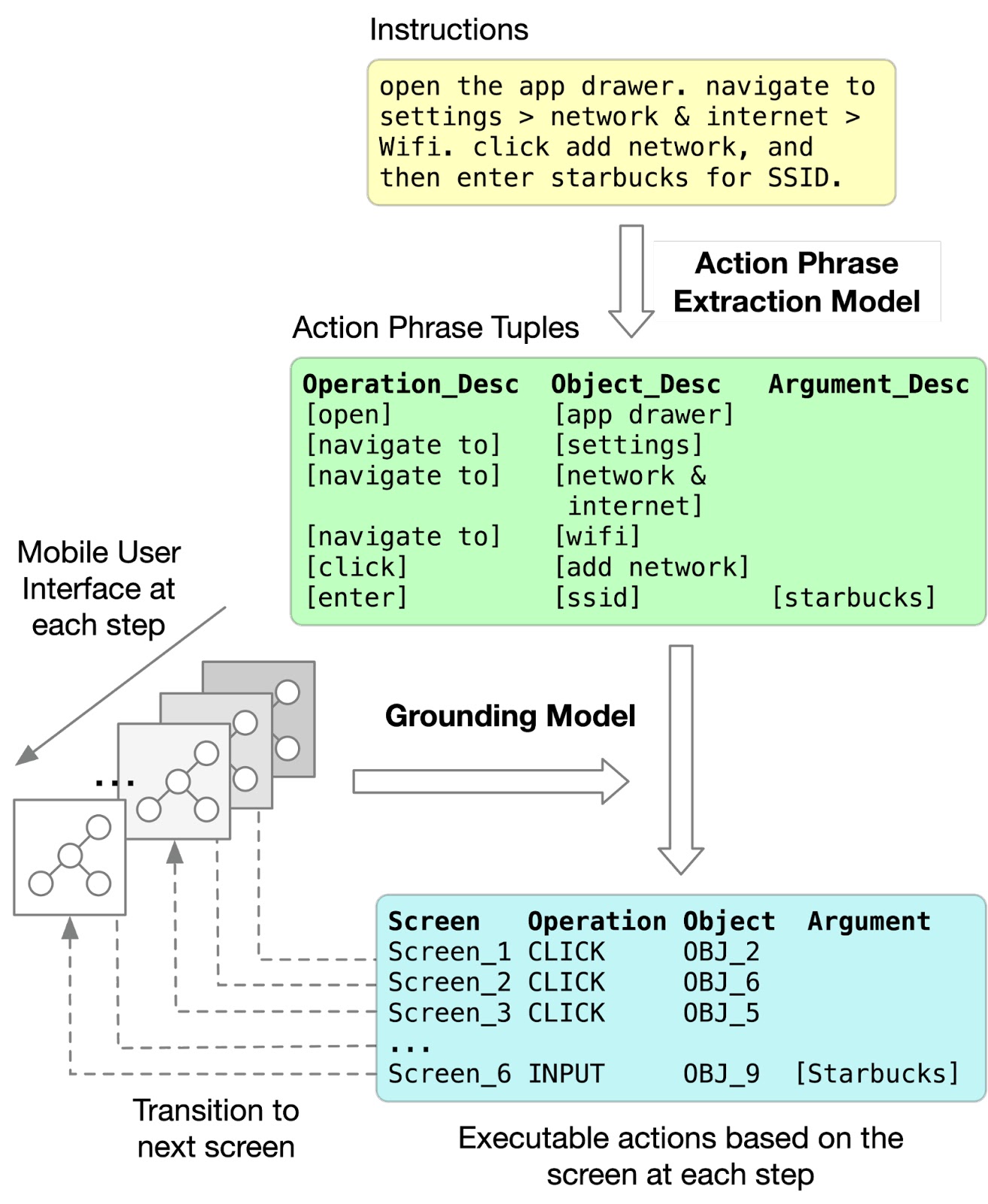
The workflow of grounding language instructions to executable actions.
The action phrase-extraction step identifies the operation, object and argument descriptions from multi-step instructions using a Transformer model with area attention for representing each description phrase. Area attention allows the model to attend to a group of adjacent words in the instruction (a span) as a whole for decoding a description.
The action phrase extraction model takes a word sequence of a natural language instruction and outputs a sequence of spans (denoted in red boxes) that indicate the phrases describing the operation, the object and the argument of each action in the task.
Next, the grounding step matches the extracted operation and object descriptions with a UI object on the screen. Again, we use a Transformer model, but in this case, it contextually represents UI objects and grounds object descriptions to them.
The grounding model takes the extracted spans as input and grounds them to executable actions, including the object an action is applied to, given the UI screen at each step during execution.
Results
To investigate the feasibility of this task and the effectiveness of our approach, we construct three new datasets to train and evaluate our model. The first dataset includes 187 multi-step English instructions for operating Pixel phones along their corresponding action-screen sequences and enables assessment of full task performance on naturally occurring instructions, which is used for testing end-to-end grounding quality. For action phrase extraction training and evaluation, we obtain English “how-to” instructions that can be found abundantly from the web and annotate phrases that describe each action. To train the grounding model, we synthetically generate 295K single-step commands to UI actions, covering 178K different UI objects across 25K mobile UI screens from a public android UI corpus.

A Transformer with area attention obtains 85.56% accuracy for predicting span sequences that completely match the ground truth. The phrase extractor and grounding model together obtain 89.21% partial and 70.59% complete accuracy for matching ground-truth action sequences on the more challenging task of mapping language instructions to executable actions end-to-end. We also evaluated alternative methods and representations of UI objects, such as using a graph convolutional network (GCN) or a feedforward network, and found those that can represent an object contextually in the screen lead to better grounding accuracy. The new datasets, models and results provide an important first step on the challenging problem of grounding natural language instructions to mobile UI actions.

Conclusion
This research, and language grounding in general, is an important step for translating multi-stage instructions into actions on a graphical user interface. Successful application of task automation to the UI domain has the potential to significantly improve accessibility, where language interfaces might help individuals who are visually impaired perform tasks with interfaces that are predicated on sight. This also matters for situational impairment when one cannot access a device easily while encumbered by tasks at hand.

By deconstructing the problem into action phrase extraction and language grounding, progress on either can improve full task performance and it alleviates the need to have language-action paired datasets, which are difficult to collect at scale. For example, action span extraction is related to both semantic role labeling and extraction of multiple facts from text and could benefit from innovations in span identification and multitask learning. Reinforcement learning that has been applied in previous grounding work may help improve out-of-sample prediction for grounding in UIs and improve direct grounding from hidden state representations. Although our datasets were based on Android UIs, our approach can be applied generally to instruction grounding on other user interface platforms. Lastly, our work provides a technical foundation for investigating user experiences in language-based human computer interaction.

Acknowledgements
Many thanks to my collaborators on this work at Google Research. Xin Zhou and Jiacong He contributed substantially to the data pipelines and the creation of the datasets. Yuan Zhang and Jason Baldridge provided much valuable advice for the project and contributed to the presentation of the work. Gang Li provided generous help for creating open-source datasets. Many thanks to Ashwin Kakarla, Muqthar Mohammad and Mohd Majeed for their help with the annotations.

Source: Google AI Blog


Machine Learning-based Damage Assessment for Disaster Relief


Natural disasters, such as earthquakes, hurricanes, and floods, affect large areas and millions of people, but responding to such disasters is a massive logistical challenge. Crisis responders, including governments, NGOs, and UN organizations, need fast access to comprehensive and accurate assessments in the aftermath of disasters to plan how best to allocate limited resources.To this end, very high resolution (VHR) satellite imagery, with up to 0.3 meter resolution, is becoming an increasingly important tool for crisis response, giving responders an unprecedented breadth of visual information about how terrain, infrastructure, and populations are changed by disasters.

However, intensive manual labor is still required to extract operationally-relevant information — collapsed buildings, cracks in bridges, where people have set up temporary shelters — from the raw satellite imagery. As an example, for the 2010 Haiti earthquake, analysts manually examined over 90,000 buildings in the Port-au-Prince area alone, rating the damage each one incurred on a five point scale. Many of these manual analyses take teams of experts many weeks to complete, whereas they are most needed within 48-72 hours after the disaster, when the most urgent decisions are made.

To help mitigate the impact of such disasters, we present "Building Damage Detection in Satellite Imagery Using Convolutional Neural Networks", which details a machine learning (ML) approach to automatically process satellite data to generate building damage assessments. Developed in partnership with the United Nations World Food Program (WFP) Innovation Accelerator, we believe this work has the potential to drastically reduce the time and effort required for crisis workers to produce damage assessment reports. In turn, this would reduce the turnaround times needed to deliver timely disaster aid to the most severely affected areas, while increasing the overall coverage of such critical services.

The Approach
The automatic damage assessment process is split into two steps: building detection and damage classification. In the building detection step, our approach uses an object detection model to draw bounding boxes around each building in the image. We then extract pre-disaster and post-disaster images centered on each detected building and use a classification model to determine whether the building is damaged.

The classification model consists of a convolutional neural network to which is input two 161 pixel x 161 pixel RGB images, corresponding to a 50 m x 50 m ground footprint, centered on a given building. One image is from before the disaster event, and the other image is from after the disaster event. The model analyzes differences in the two images and outputs a score from 0.0 to 1.0, where 0.0 means the building was not damaged, and 1.0 means the building was damaged.

Because the before and after images are taken on different dates, at different times of day, and in some cases by different satellites altogether, there can be a host of different problems that arise. For example, the brightness, contrast, color saturation, and lighting conditions of the images may differ significantly, and the pixels in the image may be misaligned.

To correct for differences in color and illumination, we use histogram equalization to normalize the colors in the before and after images. We also make the model more robust to insignificant color differences by using standard data augmentation techniques, such as randomly perturbing the contrast and saturation of the images, during training.

Training Data
One of the main challenges of this work is assembling a training data set. Data availability in this application is inherently limited because there are only a handful of disasters that have high resolution satellite images and an even smaller number that have existing damage assessments. For labels, we use publicly available damage assessments manually generated by humanitarian organizations operating in this space, such as UNOSAT and REACH. We obtain the original satellite images on which the manual assessments are performed and then use Google Earth Engine to spatially join the damage assessment labels with the satellite images in order to produce the final training examples. All images used to train the model were sourced from commercially available sources.
Examples of individual image patches that capture before and after images of damaged and undamaged buildings from different disasters.
Results
We evaluated this technology for 3 major past earthquakes: the 2010 earthquake in Haiti (magnitude 7.0), the 2017 event in Mexico City (magnitude 7.1), and the series of earthquakes occuring in Indonesia in 2018 (magnitudes 5.9 - 7.5). For each event, we trained the model on buildings in one part of the region affected by the quake and tested it on buildings in another part of the region. We used human expert damage assessments performed by UNOSAT and REACH as the ground truth for evaluation. We measure the model’s quality using both true accuracy (compared to expert assessment) and the area under the ROC curve (AUROC), which captures the trade-off between the model’s true positive and false positive rates of detection, and is a common way to measure quality when the number of positive and negative examples in the test dataset is imbalanced. An AUROC value of 0.5 means that the model’s predictions are random, while a value of 1.0 means the model is perfectly accurate. According to crisis responder feedback, 70% accuracy is the threshold needed for making high-level decisions in the first 72 hours after the disaster.
Area under the
Event Accuracy ROC curve
2010 Haiti earthquake 77% 0.83
2017 Mexico City earthquake 71% 0.79
2018 Indonesia earthquake 78% 0.86
Evaluation of model predictions against human expert assessments (higher is better).
Example model predictions from the 2010 Haiti earthquake. Prediction values closer to 1.0 means the model is more confident that the building is damaged. Values closer to 0.0 means the building is not damaged. A threshold value of 0.5 is typically used to distinguish between damaged/undamaged predictions, but this can be tuned to make the predictions more or less sensitive.
Future Work
While the current model works reasonably well when trained and tested on buildings from the same regions (e.g., same city or country), the ultimate goal is to have a model that can accurately assess building damage for disasters that happen anywhere in the world, and not just those that look similar to the ones the model has been trained on. This is challenging because the variety of the available training data for past disasters is inherently limited to a handful of events that occurred in a few geographic locations. Generalizing to future disasters that will likely occur in new locations is therefore still a challenge for our model and is the focus of ongoing work. We envision a system that can be interactively trained, validated, and deployed by expert analysts so that important aid distribution decisions are always verified by experienced crisis responders. Our hope is that this technology can help communities get the aid that they need in times of most critical need in a timely fashion.

Acknowledgements
This post reflects the work of our co-authors Wenhan Lu and Zebo Li. We would also like to thank Maolin Zuo for his contributions to the project. In tackling this problem, we have had a very productive partnership with the United Nations World Food Programme (WFP) Innovation Accelerator, an organization that identifies, funds, and supports startups and innovative projects to disrupt world hunger.

Source: Google AI Blog


Open-Sourcing BiT: Exploring Large-Scale Pre-training for Computer Vision


A common refrain for computer vision researchers is that modern deep neural networks are always hungry for more labeled data — current state-of-the-art CNNs need to be trained on datasets such as OpenImages or Places, which consist of over 1M labelled images. However, for many applications, collecting this amount of labeled data can be prohibitive to the average practitioner.

A common approach to mitigate the lack of labeled data for computer vision tasks is to use models that have been pre-trained on generic data (e.g., ImageNet). The idea is that visual features learned on the generic data can be re-used for the task of interest. Even though this pre-training works reasonably well in practice, it still falls short of the ability to both quickly grasp new concepts and understand them in different contexts. In a similar spirit to how BERT and T5 have shown advances in the language domain, we believe that large-scale pre-training can advance the performance of computer vision models.

In “Big Transfer (BiT): General Visual Representation Learning” we devise an approach for effective pre-training of general features using image datasets at a scale beyond the de-facto standard (ILSVRC-2012). In particular, we highlight the importance of appropriately choosing normalization layers and scaling the architecture capacity as the amount of pre-training data increases. Our approach exhibits unprecedented performance adapting to a wide range of new visual tasks, including the few-shot recognition setting and the recently introduced “real-world” ObjectNet benchmark. We are excited to share the best BiT models pre-trained on public datasets, along with code in TF2, Jax, and PyTorch. This will allow anyone to reach state-of-the-art performance on their task of interest, even with just a handful of labeled images per class.

Pre-training
In order to investigate the effect of data scale, we revisit common design choices of the pre-training setup (such as normalizations of activations and weights, model width/depth and training schedules) using three datasets: ILSVRC-2012 (1.28M images with 1000 classes), ImageNet-21k (14M images with ~21k classes) and JFT (300M images with ~18k classes). Importantly, with these datasets we concentrate on the previously underexplored large data regime.

We first investigate the interplay between dataset size and model capacity. To do this we train classical ResNet architectures, which perform well, while being simple and reproducible. We train variants from the standard 50-layer deep “R50x1” up to the 4x wider and 152-layer deep “R152x4” on each of the above-mentioned datasets. A key observation is that in order to profit from more data, one also needs to increase model capacity. This is exemplified by the red arrows in the left-hand panel of the figure below
Left: In order to make effective use of a larger dataset for pre-training, one needs to increase model capacity. The red arrows exemplify this: small architectures (smaller point) become worse when pre-trained on the larger ImageNet-21k, whereas the larger architectures (larger points) improve. Right: Pre-training on a larger dataset alone does not necessarily result in improved performance, e.g., when going from ILSVRC-2012 to the relatively larger ImageNet-21k. However, by also increasing the computational budget and training for longer, the performance improvement is pronounced.
A second, even more important observation, is that the training duration becomes crucial. If one pre-trains on a larger dataset without adjusting the computational budget and training longer, performance is likely to become worse. However, by adapting the schedule to the new dataset, the improvements can be significant.

During our exploration phase, we discovered another modification crucial to improving performance. We show that replacing batch normalization (BN, a commonly used layer that stabilizes training by normalizing activations) with group normalization (GN) is beneficial for pre-training at large scale. First, BN’s state (mean and variance of neural activations) needs adjustment between pre-training and transfer, whereas GN is stateless, thus side-stepping this difficulty. Second, BN uses batch-level statistics, which become unreliable with small per-device batch sizes that are inevitable for large models. Since GN does not compute batch-level statistics, it also side-steps this issue. For more technical details, including the use of a weight standardization technique to ensure stable behavior, please see our paper.
Summary of our pre-training strategy: take a standard ResNet, increase depth and width, replace BatchNorm (BN) with GroupNorm and Weight Standardization (GNWS), and train on a very large and generic dataset for many more iterations.
Transfer Learning
Following the methods established in the language domain by BERT, we fine-tune the pre-trained BiT model on data from a variety of “downstream” tasks of interest, which may come with very little labeled data. Because the pre-trained model already comes with a good understanding of the visual world, this simple strategy works remarkably well.

Fine-tuning comes with a lot of hyper-parameters to be chosen, such as learning-rate, weight-decay, etc. We propose a heuristic for selecting these hyper-parameters that we call “BiT-HyperRule”, which is based only on high-level dataset characteristics, such as image resolution and the number of labeled examples. We successfully apply the BiT-HyperRule on more than 20 diverse tasks, ranging from natural to medical images.
Once the BiT model is pre-trained, it can be fine-tuned on any task, even if only few labeled examples are available.
When transfering BiT to tasks with very few examples, we observe that as we simultaneously increase the amount of generic data used for pre-training and the architecture capacity, the ability of the resulting model to adapt to novel data drastically improves. On both 1-shot and 5-shot CIFAR (see Fig below) increasing model capacity yields limited returns when pre-training on ILSVRC (green curves). Yet, with large-scale pre-training on JFT, each step-up in model capacity yields massive returns (brown curves), up to BiT-L which attains 64% 1-shot and 95% 5-shot.
The curves depict median accuracy over 5 independent runs (light points) when transferring to CIFAR-10 with only 1 or 5 images per class (10 or 50 images total). It is evident that large architectures pre-trained on large datasets are significantly more data-efficient.
In order to verify that this result holds more generally, we also evaluate BiT on VTAB-1k, which is a suite of 19 diverse tasks with only 1000 labeled examples per task. We transfer the BiT-L model to all these tasks and achieve a score of 76.3% overall, which is a 5.8% absolute improvement over the previous state-of-the-art.

We show that this strategy of large-scale pre-training and simple transfer is effective even when a moderate amount of data is available by evaluating BiT-L on several standard computer vision benchmarks such as Oxford Pets and Flowers, CIFAR, etc. On all of these, BiT-L matches or surpasses state-of-the-art results. Finally, we use BiT as a backbone for RetinaNet on the MSCOCO-2017 detection task and confirm that even for such a structured output task, using large-scale pre-training helps considerably.
Left: Accuracy of BiT-L compared to the previous state-of-the-art general model on various standard computer vision benchmarks. Right: Results in average precision (AP) of using BiT as backbone for RetinaNet on MSCOCO-2017.
It is important to emphasize that across all the different downstream tasks we consider, we do not perform per-task hyper-parameter tuning and rely on the BiT-HyperRule. As we show in the paper, even better results can be achieved by tuning hyperparameters on sufficiently large validation data.

Evaluation on “Real-World” Images (ObjectNet)
To further assess the robustness of BiT in a more challenging scenario, we evaluate BiT models that were fine-tuned on ILSVRC-2012 on the recently introduced ObjectNet dataset. This dataset closely resembles real-world scenarios, where objects may appear in atypical context, viewpoint, rotation, etc. Interestingly, the benefit from data and architecture scale is even more pronounced with the BiT-L model achieving unprecedented top-5 accuracy of 80.0%, an almost 25% absolute improvement over the previous state-of-the-art.
Results of BiT on the ObjectNet evaluation dataset. Left: top-5 accuracy, right: top-1 accuracy.
Conclusion
We show that given pre-training on large amounts of generic data, a simple transfer strategy leads to impressive results, both on large datasets as well as tasks with very little data, down to a single image per class. We release the BiT-M model, a R152x4 pre-trained on ImageNet-21k, along with colabs for transfer in Jax, TensorFlow2, and PyTorch. We hope that practitioners and researchers find it a useful alternative to commonly used ImageNet pre-trained models.

Acknowledgements
We would like to thank Xiaohua Zhai, Joan Puigcerver, Jessica Yung, Sylvain Gelly, and Neil Houlsby who have co-authored the BiT paper and been involved in all aspects of its development, as well as the Brain team in Zürich. We also would like to thank Andrei Giurgiu for his help in debugging input pipelines. We thank Tom Small for creating the animations used in this blogpost. Finally, we refer the interested reader to the related approaches in this direction by our colleagues in Google Research, Noisy Student, as well as Facebook Research’s highly relevant Exploring the Limits of Weakly Supervised Pretraining.

Source: Google AI Blog


Announcing Meta-Dataset: A Dataset of Datasets for Few-Shot Learning


Recently, deep learning has achieved impressive performance on an array of challenging problems, but its success often relies on large amounts of manually annotated training data. This limitation has sparked interest in learning from fewer examples. A well-studied instance of this problem is few-shot image classification: learning new classes from only a few representative images.

In addition to being an interesting problem from a scientific perspective due to the apparent gap between the ability of a person to learn from limited information compared to that of a deep learning algorithm, few-shot classification is also a very important problem from a practical perspective. Because large labeled datasets are often unavailable for tasks of interest, solving this problem would enable, for example, quick customization of models to individual user’s needs, democratizing the use of machine learning. Indeed, there has been an explosion of recent work to tackle few-shot classification, but previous benchmarks fail to reliably assess the relative merits of the different proposed models, inhibiting research progress.

In “Meta-Dataset: A Dataset of Datasets for Learning to Learn from Few Examples” (presented at ICLR 2020), we propose a large-scale and diverse benchmark for measuring the competence of different image classification models in a realistic and challenging few-shot setting, offering a framework in which one can investigate several important aspects of few-shot classification. It is composed of 10 publicly available datasets of natural images (including ImageNet, CUB-200-2011, Fungi, etc.), handwritten characters and doodles. The code is public, and includes a notebook that demonstrates how Meta-Dataset can be used in TensorFlow and PyTorch. In this blog post, we outline some results from our initial research investigation on Meta-Dataset and highlight important research directions.

Background: Few-shot Classification
In standard image classification, a model is trained on a set of images from a particular set of classes, and then tested on a held-out set of images of those same classes. Few-shot classification goes a step further and studies generalization to entirely new classes at test time, no images of which were seen in training.

Specifically, in few-shot classification, the training set contains classes that are entirely disjoint from those that will appear at test time. So the aim of training is to learn a flexible model that can be easily repurposed towards classifying new classes using only a few examples. The end-goal is to perform well on the test-time evaluation that is carried out on a number of test tasks, each of which presents a classification problem between previously unseen classes, from a held out test set of classes. Each test task contains a support set of a few labeled images from which the model can learn about the new classes, and a disjoint query set of examples that the model is then asked to classify.

In Meta-Dataset, in addition to the tough generalization challenge to new classes inherent in the few-shot learning setup described above, we also study generalization to entirely new datasets, from which no images of any class were seen in training.

Comparison of Meta-Dataset with Previous Benchmarks
A popular dataset for studying few-shot classification is mini-ImageNet, a downsampled version of a subset of classes from ImageNet. This dataset contains 100 classes in total that are divided into training, validation and test class splits. While classes encountered at test time in benchmarks like mini-ImageNet have not been seen during training, they are still substantially similar to the training classes visually. Recent works reveal that this allows a model to perform competitively at test time simply by re-using features learned at training time, without necessarily demonstrating the capability to learn from the few examples presented to the model in the support set. In contrast, performing well on Meta-Dataset requires absorbing diverse information at training time and rapidly adapting it to solve significantly different tasks at test time that possibly originate from entirely unseen datasets.
Test tasks from mini-ImageNet. Each task is a classification problem between previously unseen (test) classes. The model can use the support set of a few labeled examples of the new classes to adapt to the task at hand and then predicts labels for the query examples of these new classes. The evaluation metric is the query set accuracy, averaged over examples within each task and across tasks.
While other recent papers have investigated training on mini-ImageNet and evaluating on different datasets, Meta-Dataset represents the largest-scale organized benchmark for cross-dataset, few-shot image classification to date. It also introduces a sampling algorithm for generating tasks of varying characteristics and difficulty, by varying the number of classes in each task, the number of available examples per class, introducing class imbalances and, for some datasets, varying the degree of similarity between the classes of each task. Some example test tasks from Meta-Dataset are shown below.
Test tasks from Meta-Dataset. Contrary to the mini-ImageNet tasks shown above, different tasks here originate from (the test classes of) different datasets. Further, the number of classes and the support set sizes differ across tasks and the support sets might be class-imbalanced.
Initial Investigation and Findings on Meta-Dataset
We benchmark two main families of few-shot learning models on Meta-Dataset: pre-training and meta-learning.

Pre-training simply trains a classifier (a neural network feature extractor followed by a linear classifier) on the training set of classes using supervised learning. Then, the examples of a test task can be classified either by fine-tuning the pre-trained feature extractor and training a new task-specific linear classifier, or by means of nearest-neighbor comparisons, where the prediction for each query example is the label of its nearest support example. Despite its “baseline” status in the few-shot classification literature, this approach has recently enjoyed a surge of attention and competitive results.

On the other hand, meta-learners construct a number of “training tasks” and their training objective explicitly reflects the goal of performing well on each task’s query set after having adapted to that task using the associated support set, capturing the ability that is required at test time to solve each test task. Each training task is created by randomly sampling a subset of training classes and some examples of those classes to play the role of support and query sets.

Below, we summarize some of our findings from evaluating pre-training and meta-learning models on Meta Dataset:

1) Existing approaches have trouble leveraging heterogeneous training data sources.

We compared training models (from both pre-training and meta-learning approaches) using only the training classes of ImageNet to using all training classes from the datasets in Meta-Dataset, in order to measure the generalization gain from using a more expansive collection of training data. We singled out ImageNet for this purpose, because the features learned on ImageNet readily transfer to other datasets. The evaluation tasks applied to all models are derived from a held-out set of classes from the datasets used in training, with at least two additional datasets that are entirely held-out for evaluation (i.e., no classes from these datasets were used for training).

One might expect that training on more data, albeit heterogeneous, would generalize better on the test set. However, this is not always the case. Specifically, the following figure displays the accuracy of different models on test tasks of Meta-Dataset’s ten datasets. We observe that the performance on test tasks coming from handwritten characters / doodles (Omniglot and Quickdraw) is significantly improved when having trained on all datasets, instead of ImageNet only. This is reasonable since these datasets are visually significantly different from ImageNet. However, for test tasks of natural image datasets, similar accuracy can be obtained by training on ImageNet only, revealing that current models cannot effectively leverage heterogeneous data towards improving in this regard.
Comparison of test performance on each dataset after having trained on ImageNet (ILSVRC-2012) only or on all datasets.
2) Some models are more capable than others of exploiting additional data at test time.

We analyzed the performance of different models as a function of the number of available examples in each test task, uncovering an interesting trade-off: different models perform best with a particular number of training (support) samples. We observe that some models outshine the rest when there are very few examples (“shots”) available (e.g., ProtoNet and our proposed fo-Proto-MAML) but don’t exhibit a large improvement when given more, while other models are not well-suited for tasks with very few examples but improve at a quicker rate as more are given (e.g., Finetune baseline). However, since in practice we might not know in advance the number of examples that will be available at test time, one would like to identify a model that can best leverage any number of examples, without disproportionately suffering in a particular regime.
Comparison of test performance averaged across different datasets to the number of examples available per class in test tasks (“shots”). Performance is measured in terms of class precision: the proportion of the examples of a class that are correctly labeled, averaged across classes.
3) The adaptation algorithm of a meta-learner is more heavily responsible for its performance than the fact that it is trained end-to-end (i.e. meta-trained).

We developed a new set of baselines to measure the benefit of meta-learning. Specifically, for several meta-learners, we consider a non-meta-learned counterpart that pre-trains a feature extractor and then, at evaluation time only, applies the same adaptation algorithm as the respective meta-learner on those features. When training on ImageNet only, meta-training often helps a bit or at least doesn’t hurt too much, but when training on all datasets, the results are mixed. This suggests that further work is needed to understand and improve upon meta-learning, especially across datasets.
Comparison of three different meta-learner variants to their corresponding inference-only baselines, when training on ImageNet (ILSVRC-1012) only or all datasets. Each bar represents the difference between meta-training and inference-only, so positive values indicate improved performance from meta-training.
Conclusion
Meta-Dataset introduces new challenges for few-shot classification. Our initial exploration has revealed limitations of existing methods, calling for additional research. Recent works have already reported exciting results on Meta-Dataset, for example using cleverly-designed task conditioning, more sophisticated hyperparameter tuning, a ‘meta-baseline’ that combines the benefits of pre-training and meta-learning, and finally using feature selection to specialize a universal representation for each task. We hope that Meta-Dataset will help drive research in this important sub-field of machine learning.

Acknowledgements
Meta-Dataset was developed by Eleni Triantafillou, Tyler Zhu, Vincent Dumoulin, Pascal Lamblin, Utku Evci, Kelvin Xu, Ross Goroshin, Carles Gelada, Kevin Swersky, Pierre-Antoine Manzagol and Hugo Larochelle. We would like to thank Pablo Castro for his valuable guidance on this blog post, Chelsea Finn for fruitful discussions and ensuring the correctness of fo-MAML’s implementation, as well as Zack Nado and Dan Moldovan for the initial dataset code that was adapted, Cristina Vasconcelos for spotting an issue in the ranking of models and John Bronskill for suggesting that we experiment with a larger inner-loop learning rate for MAML which indeed significantly improved our fo-MAML results.

Source: Google AI Blog


Speeding Up Neural Network Training with Data Echoing


Over the past decade, dramatic increases in neural network training speed have made it possible to apply deep learning techniques to many important problems. In the twilight of Moore's law, as improvements in general purpose processors plateau, the machine learning community has increasingly turned to specialized hardware to produce additional speedups. For example, GPUs and TPUs optimize for highly parallelizable matrix operations, which are core components of neural network training algorithms. These accelerators, at a high level, can speed up training in two ways. First, they can process more training examples in parallel, and second, they can process each training example faster. We know there are limits to the speedups from processing more training examples in parallel, but will building ever faster accelerators continue to speed up training?

Unfortunately, not all operations in the training pipeline run on accelerators, so one cannot simply rely on faster accelerators to continue driving training speedups. For example, earlier stages in the training pipeline like disk I/O and data preprocessing involve operations that do not benefit from GPUs and TPUs. As accelerator improvements outpace improvements in CPUs and disks, these earlier stages will increasingly become a bottleneck, wasting accelerator capacity and limiting training speed.
An example training pipeline representative of many large-scale computer vision programs. The stages that come before applying the mini-batch stochastic gradient descent (SGD) update generally do not benefit from specialized hardware accelerators.
Consider a scenario where the code upstream to the accelerator takes twice as long as the code that runs on the accelerator – a scenario that is already realistic for some workloads today. Even if the code is pipelined to execute the upstream and downstream stages in parallel, the upstream stage will dominate training time and the accelerator will be idle 50% of the time. In this case, building a faster accelerator will not improve training speed at all. It may be possible to speed up the input pipeline by dedicating engineering effort and additional compute resources, but such efforts are time consuming and distract from the main goal of improving predictive performance. For very small datasets,one can precompute the augmented dataset offline and load the entire preprocessed dataset in memory, but this doesn’t work for most ML training scenarios.

In “Faster Neural Network Training with Data Echoing”, we propose a simple technique that reuses (or “echoes”) intermediate outputs from earlier pipeline stages to reclaim idle accelerator capacity. Rather than waiting for more data to become available, we simply utilize data that is already available to keep the accelerators busy.
Left: Without data echoing, downstream computational capacity is idle 50% of the time. Right: Data echoing with echoing factor 2 reclaims downstream computational capacity.
Repeating Data to Train Faster
Imagine a situation where reading and preprocessing a batch of training data takes twice as long as performing a single optimization step on that batch. In this case, after the first optimization step on the preprocessed batch, we can reuse the batch and perform a second step before the next batch is ready. In the best case scenario, where repeated data is as useful as fresh data, we would see a twofold speedup in training. In reality, data echoing provides a slightly smaller speedup because repeated data is not as useful as fresh data – but it can still provide a significant speedup compared to leaving the accelerator idle.

There are typically several ways to implement data echoing in a given neural network training pipeline. The technique we propose involves duplicating data into a shuffle buffer somewhere in the training pipeline, but we are free to insert this buffer anywhere after whichever stage produces a bottleneck in the given pipeline. When we insert the buffer before batching, we call our technique example echoing, whereas, when we insert it after batching, we call our technique batch echoing. Example echoing shuffles data at the example level, while batch echoing shuffles the sequence of duplicate batches. We can also insert the buffer before data augmentation, such that each copy of repeated data is slightly different (and therefore closer to a fresh example). Of the different versions of data echoing that place the shuffle buffer between different stages, the version that provides the greatest speedup depends on the specific training pipeline.

Data Echoing Across Workloads
So how useful is reusing data? We tried data echoing on five neural network training pipelines spanning 3 different tasks – image classification, language modeling, and object detection – and measured the number of fresh examples needed to reach a particular performance target. We chose targets to match the best result reliably achieved by the baseline during hyperparameter tuning. We found that data echoing allowed us to reach the target performance with fewer fresh examples, demonstrating that reusing data is useful for reducing disk I/O across a variety of tasks. In some cases, repeated data is nearly as useful as fresh data: in the figure below, example echoing before augmentation reduces the number of fresh examples required almost by the repetition factor.
Data echoing, when each data item is repeated twice, either reduces or does not change the number of fresh examples needed to reach the target out-of-sample performance. Dashed lines indicate the values we would expect if repeated examples were as useful as fresh examples.
Reduction in Training Time
Data echoing can speed up training whenever computation upstream from accelerators dominates training time. We measured the training speedup achieved in a training pipeline bottlenecked by input latency due to streaming training data from cloud storage, which is realistic for many of today’s large-scale production workloads or anyone streaming training data over a network from a remote storage system. We trained a ResNet-50 model on the ImageNet dataset and found that data echoing provides a significant training speedup, in this case, more than 3 times faster when using data echoing.
Data echoing can reduce training time for ResNet-50 on ImageNet. In this experiment, reading a batch of training data from cloud storage took 6 times longer than the code that used each batch of data to perform a training step. The Echoing factor in the legend refers to the number of times each data item was repeated. Dashed lines indicate the expected values if repeated examples were as useful as fresh examples and there was no overhead from echoing.
Data Echoing Preserves Predictive Performance
Although one might be concerned that reusing data would harm the model’s final performance, we found that data echoing did not degrade the quality of the final model for any of the workloads we tested.
Comparing the individual trials that achieved the best out-of-sample performance during training for both with and without data echoing shows that reusing data does not harm final model quality. Here validation cross entropy is equivalent to log perplexity.
As improvements in specialized accelerators like GPUs and TPUs continue to outpace general purpose processors, we expect data echoing and similar strategies to become increasingly important parts of the neural network training toolkit.

Acknowledgements
The Data Echoing project was conducted by Dami Choi, Alexandre Passos, Christopher J. Shallue, and George E. Dahl while Dami Choi was a Google AI Resident. We would also like to thank Roy Frostig, Luke Metz, Yiding Jiang, and Ting Chen for helpful discussions.

Source: Google AI Blog


Optimizing Multiple Loss Functions with Loss-Conditional Training


In many machine learning applications the performance of a model cannot be summarized by a single number, but instead relies on several qualities, some of which may even be mutually exclusive. For example, a learned image compression model should minimize the compressed image size while maximizing its quality. It is often not possible to simultaneously optimize all the values of interest, either because they are fundamentally in conflict, like the image quality and the compression ratio in the example above, or simply due to the limited model capacity. Hence, in practice one has to decide how to balance the values of interest.
The trade-off between the image quality and the file size in image compression. Ideally both the image distortion and the file size would be minimized, but these two objectives are fundamentally in conflict.
The standard approach to training a model that must balance different properties is to minimize a loss function that is the weighted sum of the terms measuring those properties. For instance, in the case of image compression, the loss function would include two terms, corresponding to the image reconstruction quality and the compression rate. Depending on the coefficients on these terms, training with this loss function results in a model producing image reconstructions that are either more compact or of higher quality.

If one needs to cover different trade-offs between model qualities (e.g. image quality vs compression rate), the standard practice is to train several separate models with different coefficients in the loss function of each. This requires keeping around multiple models both during training and inference, which is very inefficient. However, all of these separate models solve very related problems, suggesting that some information could be shared between them.

In two concurrent papers accepted at ICLR 2020, we propose a simple and broadly applicable approach that avoids the inefficiency of training multiple models for different loss trade-offs and instead uses a single model that covers all of them. In “You Only Train Once: Loss-Conditional Training of Deep Networks”, we give a general formulation of the method and apply it to several tasks, including variational autoencoders and image compression, while in “Adjustable Real-time Style Transfer”, we dive deeper into the application of the method to style transfer.

Loss-Conditional Training
The idea behind our approach is to train a single model that covers all choices of coefficients of the loss terms, instead of training a model for each set of coefficients. We achieve this by (i) training the model on a distribution of losses instead of a single loss function, and (ii) conditioning the model outputs on the vector of coefficients of the loss terms. This way, at inference time the conditioning vector can be varied, allowing us to traverse the space of models corresponding to loss functions with different coefficients.

This training procedure is illustrated in the diagram below for the style transfer task. For each training example, first the loss coefficients are randomly sampled. Then they are used both to condition the main network via the conditioning network and to compute the loss. The whole system is trained jointly end-to-end, i.e., the model parameters are trained concurrently with random sampling of loss functions.
Overview of the method, using stylization as an example. The main stylization network is conditioned on randomly sampled coefficients of the loss function and is trained on a distribution of loss functions, thus learning to model the entire family of loss functions.
The conceptual simplicity of this approach makes it applicable to many problem domains, with only minimal changes to existing code bases. Here we focus on two such applications, image compression and style transfer.

Application: Variable-Rate Image Compression
As a first example application of our approach, we show the results for learned image compression. When compressing an image, a user should be able to choose the desired trade-off between the image quality and the compression rate. Classic image compression algorithms are designed to allow for this choice. Yet, many leading learned compression methods require training a separate model for each such trade-off, which is computationally expensive both at training and at inference time. For problems such as this, where one needs a set of models optimized for different losses, our method offers a simple way to avoid inefficiency and cover all trade-offs with a single model.

We apply the loss-conditional training technique to the learned image compression model of Balle et al. The loss function here consists of two terms, a reconstruction term responsible for the image quality and a compactness term responsible for the compression rate. As illustrated below, our technique allows training a single model covering a wide range of quality-compression tradeoffs.
Compression at different quality levels with a single model. All animations are generated with a single model by varying the conditioning value.
Application: Adjustable Style Transfer
The second application we demonstrate is artistic style transfer, in which one synthesizes an image by merging the content from one image and the style from another. Recent methods allow training deep networks that stylize images in real time and in multiple styles. However, for each given style these methods do not allow the user to have control over the details of the synthesized output, for instance, how much to stylize the image and on which style features to place greater emphasis. If the stylized output is not appealing to the user, they have to train multiple models with different hyper-parameters until they get a favorite stylization.

Our proposed method instead allows training a single model covering a wide range of stylization variants. In this task, we condition the model on a loss function, which has coefficients corresponding to five loss terms, including the content loss and four terms for the stylization loss. Intuitively, the content loss regulates how much the stylized image should be similar to the original content, while the four stylization losses define which style features get carried over to the final stylized image. Below we show the outputs of our single model when varying all these coefficients:
Adjustable style transfer. All stylizations are generated with a single network by varying the conditioning values.
Clearly, the model captures a lot of variation within each style, such as the degree of stylization, the type of elements being added to the image, their exact configuration and locations, and more. More examples can be found on our webpage along with an interactive demo.

Conclusion
We have proposed loss-conditional training, a simple and general method that allows training a single deep network for tasks that would formerly require a large set of separately trained networks. While we have shown its application to image compression and style transfer, many more applications are possible — whenever the loss function has coefficients to be tuned, our method allows training a single model covering a wide range of these coefficients.

Acknowledgements
This blog post covers the work by multiple researchers on the Google Brain team: Mohammad Babaeizadeh, Johannes Balle, Josip Djolonga, Alexey Dosovitskiy, and Golnaz Ghiasi. This blog post would not be possible without crucial contributions from all of them. Images from the MS-COCO dataset and from unsplash.com are used for illustrations.

Source: Google AI Blog


Exploring Evolutionary Meta-Learning in Robotics


Rapid development of more accurate simulator engines has given robotics researchers a unique opportunity to generate sufficient amounts of data that can be used to train robotic policies for real-world deployment. However, moving trained policies from “sim-to-real” remains one of the greatest challenges of modern robotics, due to the subtle differences encountered between the simulation and real domains, termed the “reality gap”. While some recent approaches leverage existing data, such as imitation learning and offline reinforcement learning, to prepare a policy for the reality gap, a more common approach is to simply provide more data by varying properties of the simulated environment, a process called domain randomization.

However, domain randomization can sacrifice performance for stability, as it seeks to optimize for a decent, stable policy across all tasks, but offers little room for improving the policy on a specific task. This lack of a common optimal policy between simulation and reality is frequently a problem in robotic locomotion applications, where there are varying physical forces at play, such as leg friction, body mass, and terrain differences. For example, given the same initial conditions for the robot’s position and balance, the surface type will determine the optimal policy — for an incoming flat surface encountered in simulation, the robot could accelerate to a higher speed, while for an incoming rugged and bumpy surface encountered in the real world, it should walk slowly and carefully to prevent falling.

In “Rapidly Adaptable Legged Robots via Evolutionary Meta-Learning”, we present a particular type of meta-learning based on evolutionary strategies (ES), an approach generally believed to only work well in simulation, we can effectively and efficiently adapt a policy to a real-world robot in a completely model-free manner. Compared to previous approaches for adapting meta-policies, such as standard policy gradients which do not allow sim-to-teal adaptation, ES enables a robot to quickly overcome the reality gap and adapt to dynamic changes in the real world, some of which may not be encountered in simulation. This represents the first instance of successfully using ES for on-robot adaptation.
Our algorithm quickly adapts a legged robot’s policy to dynamics changes. In this example, the battery voltage dropped from 16.8V to 10V which reduced motor power, and a 500g mass was also placed on the robot's side, causing it to turn rather than walk straight. The policy is able to adapt in only 50 episodes (or 150s of real-world data).
Meta-Learning
This research falls under the general class of meta-learning techniques, and is demonstrated on a legged robot. At a high level, meta-learning learns to solve an incoming task quickly without completely retraining from scratch, by combining past experiences with small amounts of experience from the incoming task. This is especially beneficial in the sim-to-real case, where most of the past experiences come cheaply from simulation, while a minimal, yet necessary amount of experience is generated from the real world task. The simulation experiences allow the policy to possess a general level of behavior for solving a distribution of tasks, while the real-world experiences allow the policy to fine-tune specifically to the real-world task at hand.

In order to train a policy to meta-learn, it is necessary to encourage a policy to adapt during simulation. Normally, this can be achieved by applying model-agnostic meta-learning (MAML), which searches for a meta-policy that can adapt to a specific task quickly using small amounts of task-specific data. The standard approach to computing such meta-policies is by using policy gradient methods, which seek to improve the likelihood of selecting the same action given the same state. In order to determine the likelihood of a given action, the policy must be stochastic, allowing for the action selected by the policy to have a randomized component. The real-world environment for deploying such robotic policies is also highly stochastic, as there can be slight differences in motion arising naturally, even if starting from the exact same state and action sequence. The combination of using a stochastic policy inside a stochastic environment creates two conflicting objectives:
  1. Decreasing the policy’s stochasticity may be crucial, as otherwise the high-noise problem might be exacerbated by the additional randomness from the policy’s actions.

  2. However, increasing the policy’s stochasticity may also benefit exploration, as the policy needs to use random actions to probe the type of environment to which it adapts.
These two competing objectives, which have been noted before, seek to both decrease and increase the policy’s stochasticity and may cause complications.

Evolutionary Strategies in Robotics
Instead, we resolve these challenges by applying ES-MAML, an algorithm that leverages a drastically different paradigm for high-dimensional optimization — evolutionary strategies. The ES-MAML approach updates the policy based solely on the sum of rewards collected by the agent in the environment. The function used for optimizing the policy is black-box, mapping the policy parameters directly to this reward. Unlike policy gradient methods, this approach does not need to collect state/action/reward tuples and does not need to estimate action likelihoods. This allows the use of deterministic policies and exploration based on parameter changes and avoiding the conflict between stochasticity in the policy and in the environment.

In this paradigm, querying usually involves running episodes in the simulator, but we show that ES can be applied also for episodes collected on real hardware. ES optimization can be easily distributed and also works well for training efficient compact policies, a phenomenon with profound robotic implications, since policies with fewer parameters can be easier deployed on real hardware and often lead to more efficient inference and power usage. We confirm the effectiveness of ES in training compact policies by learning adaptable meta-policies with <130 parameters.

The ES optimization paradigm is very flexible. It can be used to optimize non-differentiable objectives, such as the total reward objective in our robotics case. It also works in the presence of substantial (potentially adversarial) noise. In addition, the most recent forms of ES methods (e.g., guided ES) are much more sample-efficient than previous versions.

This flexibility is critical for efficient adaptation of locomotion meta-policies. Our results show that adaptation with ES can be conducted with a small number of additional on-robot episodes. Thus, ES is no longer just an attractive alternative to the state-of-the-art algorithms, but defines a new state of the art for several challenging RL tasks.

Adaptation in Simulation
We first examine the types of adaptation that emerge when training with ES-MAML in simulation. When testing the policy in simulation, we found that the meta-policy forces the robot to fall down when the dynamics become too unstable, whereas the adapted policy allows the robot to re-stabilize and walk again. Furthermore, when the robot’s leg settings change, the meta-policy de-synchronizes the robot’s legs causing the robot to turn sharply, while the adapted policy corrects the robot so it can walk straight again.
The meta-policy’s gait, which experiences issues when facing a difficult dynamics task. Left: The meta-policy lets the robot fall down. Center: The adapted policy ensures the robot continues to walk correctly. Right: Comparative measurement of the robot’s height.
The meta-policy’s gait, under changes to the robot’s leg settings. Left: The meta-policy allows the robot veer to the right. Center: The adapted policy ensures the robot continues to walk in a straight line. Right: Comparative measurement of the robot’s walking direction.
Adaptation in the Real World
Despite the good performance of ES-MAML in simulation, applying it to a real robot is still a challenge. To effectively adapt in the noisy environment of the real world while requiring as little real-world data as possible, we introduce batch hill-climbing, an add-on to ES-MAML based on previous work for zeroth-order blackbox optimization. Rather than performing hill-climbing which iteratively updates the input one-by-one according to a deterministic objective, batch hill-climbing samples a parallel batch of queries to determine the next input, making it robust to large amounts of noise in the objective.

We then test our method on the following 2 tasks, which are designed to significantly change the dynamics from the normal setting of the robot:
In the mass-voltage task (left), a 500g weight is placed on the robot’s side and the voltage is dropped to 10.0V from 16.8V. In the friction task (right), we replaced the rubber feet with tennis balls, to significantly reduce friction and hinder walking.
For the mass-voltage task, the initial meta-policy steered the robot significantly to the right due to the extra mass and voltage change, which caused an imbalance in the robot’s body and leg motors. However, after 30 episodes of adaptation using our method, the robot straightens the walking pose, and after 50 episodes, the robot is able to balance its body completely and is able to walk longer distances. In comparison, training from scratch on an easier, noiseless task from only simulation required approximately 90,000 episodes, showing that our method significantly reduces sample complexity on expensive real world data.
Qualitative changes during the adaptation phase under the mass-voltage task.
We compared our method to domain randomization and the standard policy gradient approach to MAML (PG-MAML) only, presenting the final policies qualitatively, as well as metrics from the real robot to show how our method adapts. We found that both domain randomization and PG-MAML baselines do not adapt as well as our method.
Comparisons between Domain Randomization and PG-MAML, and metric differences between our method’s meta-policy and adapted policy. Top: Comparison for the mass-voltage task. Our method stabilizes the robot’s roll angle. Bottom: Comparison for the friction task. Our method results in longer trajectories.
Future Work
This work exposes several avenues for future development. One option is to make algorithmic improvements to reduce the number of real-world rollouts required for adaptation. Another area for advancement is the use of model-based reinforcement learning techniques for a lifelong learning system, in which the robot can continuously collect data and quickly adjust its policy to learn new skills and to operate optimally in new environments.

Acknowledgements
This research was conducted by the core ES-MAML team: Xingyou Song, Yuxiang Yang, Krzysztof Choromanski, Ken Caluwaerts, Wenbo Gao, Chelsea Finn, and Jie Tan. We would like to give special thanks to Vikas Sindhwani for his support on ES methods, and Daniel Seita for feedback on our paper.

Source: Google AI Blog


An Optimistic Perspective on Offline Reinforcement Learning


“The potential for off-policy learning remains tantalizing, the best way to achieve it still a mystery.” — Sutton & Barto

Most reinforcement learning (RL) algorithms assume that an agent actively interacts with an online environment to learn from its own collected experience. These algorithms are challenging to apply to complex real-world problems (such as robotics and autonomous driving) since extensive data collection from the real world can be extremely sample inefficient and lead to unintended behavior, while those operating in simulation require high-fidelity simulators that are challenging to build. However, for many real-world RL applications, there already exist a large amount of previously collected interaction data which can be utilized to make RL feasible for those problems, and enable better generalization by incorporating diverse prior experiences.

Existing interaction data can be used effectively using offline RL, which is the fully off-policy RL setting in which an agent is trained from a fixed dataset of logged experiences, without any further interactions with the environment. Offline RL can help (1) pretrain an RL agent using existing data, (2) empirically evaluate RL algorithms based on their ability to utilize a fixed dataset of interactions, and (3) deliver real-world impact. However, offline RL is considered challenging due to the distribution mismatch between online interactions and any fixed dataset of logged interactions, i.e., when the learned agent takes an action different from the data collection agent, we don’t know the reward that should be provided.
RL with online interactions vs. Offline RL.
In “An Optimistic Perspective on Offline RL”, we propose a simple experimental setup for offline RL on Atari 2600 games, based on logged experiences of a DQN agent. We demonstrate that it is possible to train agents with high returns that outperform the data collection agents using standard off-policy RL algorithms, without explicitly correcting for any distribution mismatch. We also develop a robust RL algorithm, called random ensemble mixture (REM), which shows promising results on offline RL. Overall, we present an optimistic perspective that robust RL algorithms trained on sufficiently large and diverse offline datasets can lead to high quality behaviour, strengthening the emerging data-driven RL paradigm. To facilitate the development and evaluation of offline RL methods, we are also publicly releasing the DQN Replay Dataset and have open-sourced our code. More details can be found at offline-rl.github.io.

A Primer on Off-policy and Offline RL
We summarize various approaches to RL below:
Online, off-policy RL agents, such as DQN, achieve human-level performance on Atari 2600 games by just observing the game screen, without any explicit knowledge about the game. DQN estimates the effectiveness of an action at a given state of the environment in terms of maximum achievable future rewards (i.e., Q-values). Furthermore, recent distributional RL agents, such as QR-DQN, model the entire distribution of probable future rewards, rather than a single expected value for each state-action pair. Agents such as DQN and QR-DQN are considered “online” because they alternate between optimizing a policy (how an agent acts at a given state) and using that policy to collect more data.

In principle, off-policy RL agents can learn from data collected by any policy, not just the policy being optimized. However, in the offline RL setting, recent work presents a discouraging view that standard off-policy agents diverge or otherwise yield poor performance. To fix this, previous work proposes remedies by regularizing the learned policy to stay close to the dataset of offline interactions.

The DQN Replay Dataset for Offline RL
In this work, we revisit offline RL by first creating the DQN Replay Dataset. This dataset is generated using DQN agents trained on 60 Atari 2600 games for 200 million frames each, while using sticky actions (with 25% probability that the agent’s previous action is executed instead of the current action) to make the problem more challenging. For each of the 60 games, we train 5 DQN agents with different random initializations, and store all of the (state, action, reward, next state) tuples encountered during training into 5 replay datasets per game, resulting in a total of 300 datasets.
Offline RL on Atari games using the DQN Replay Dataset.
The DQN Replay Dataset can then be used for training offline RL agents, without any interaction with the environment during training. Each game replay dataset is approximately 3.5 times larger than ImageNet and includes samples from all of the intermediate policies seen during the optimization of online DQN.

Training Offline Agents on the DQN Replay Dataset
We trained offline variants of DQN and distributional QR-DQN on the DQN Replay Dataset. Although the offline datasets contain data experienced by a DQN agent improving over time as training progresses, we compared the performance of offline agents against the best performing online DQN agent obtained after training (i.e., a fully-trained DQN). For each game, we evaluated the 5 offline agents trained (one per dataset), using online returns, reporting the best averaged performance.

Offline DQN underperforms fully-trained online DQN on all except a few games, where it achieves higher scores with the same amount of data. Offline QR-DQN, on the other hand, outperforms offline DQN and fully-trained DQN on most of the games. These results demonstrate that it is possible to optimize strong agents offline using standard deep RL algorithms. Furthermore, the disparity between the performance of offline QR-DQN and DQN indicates the difference in their ability to exploit offline data.
Offline DQN. Normalized improvement over a fully-trained DQN, per game, of offline DQN trained using DQN replay. On the normalized scale, fully-trained DQN corresponds to 100% performance while random agent corresponds to 0%.
Offline QR-DQN. Normalized performance improvement (in %) over a fully-trained DQN agent, per game, of offline QR-DQN trained offline using DQN replay.
Introducing Two Robust Offline RL Agents
In online RL, an agent chooses actions that it thinks will lead to high rewards, and then receives corrective feedback. Since it is not possible to collect additional data in offline RL, it is essential to reason about generalization using a fixed dataset. Leveraging methods from supervised learning that use an ensemble of models to improve generalization, we present two new offline RL agents:
  • Ensemble-DQN is a simple extension of DQN that trains multiple Q-value estimates and averages them for evaluation.
  • Random Ensemble Mixture (REM) is an easy to implement extension of DQN inspired by Dropout. The key intuition behind REM is that if one has access to multiple estimates of Q-values, then a weighted combination of the Q-value estimates is also an estimate for Q-values. Accordingly, in each training step, REM randomly combines multiple Q-value estimates and uses this random combination for robust training.
Neural Network architectures for DQN, distributional QR-DQN and the expected RL variants with the same multi-head QR-DQN architecture, i.e., Ensemble-DQN and REM. In QR-DQN, each head (red rectangles) corresponds to a specific fraction of the return distribution, while in the proposed variants, each head approximates the Q-function.
To utilize the DQN Replay Dataset more efficiently, we train offline agents for five times as many training iterations as online DQN and report their performance below. Offline REM outperforms offline DQN and offline QR-DQN. The comparison with fully-trained online C51, a strong distributional agent, illustrates that the gains from offline REM are more than the gains from C51.
Offline REM vs. baselines. Median normalized scores averaged over 5 runs across 60 Atari games of offline agents trained using DQN replay for 5x iterations, compared to online DQN.
Using the standard training protocols on Atari, online REM performs on par with QR-DQN in the standard online RL setting. This suggests that we can use the insights gained from the DQN Replay Dataset and the offline RL setting to build effective online RL methods.
Online REM vs. baselines. Median normalized evaluation scores averaged over 5 runs (shown as traces) across stochastic 60 Atari 2600 games of online agents trained for 200 million frames. Online REM with 4 Q-networks performs comparably to online QR-DQN.
Comparison of Results: Important Factors in Offline RL
The discrepancy between these results and prior work that reports failure of standard RL agents in the offline setting could be attributed to the following factors:
  • Offline Dataset Size. We trained offline QR-DQN and REM with reduced data obtained via randomly subsampling the entire DQN Replay Dataset, maintaining the same data distribution. Analogous to supervised learning, performance tends to increase as the size of data increases. With only 10% of the entire dataset, REM and QR-DQN approximately recover the performance of fully-trained DQN.
  • Offline Dataset Composition. We trained offline RL agents on the first 20 million frames per game in the DQN Replay Dataset. Offline REM and QR-DQN outperform the best policy in this lower quality dataset, indicating that standard RL agents work well in the offline setting with sufficiently diverse datasets.
    Offline RL with Lower Quality Dataset. REM and QR-DQN trained on offline data collected from DQN trained for 20 iterations (by using the first 20M frames from each game replay dataset). The horizontal line shows the performance of best policy in this dataset, which is significantly worse than fully-trained DQN.
  • Offline Algorithm Choice. There are claims that standard off-policy agents are ineffective on continuous control tasks when trained offline. However, we found that recent continuous control agents, such as TD3, perform comparably to a sophisticated offline agent when trained on large and diverse offline datasets.
Future Work. Our results emphasize the need for a rigorous characterization of the role of generalization due to neural networks when learning from offline data collected from a large mixture of diverse policies. Benchmarking offline RL with various data collection strategies by subsampling DQN replay (e.g., first / last k million frames) is another important direction. We currently employ online policy evaluation, however, “true” offline RL requires offline policy evaluation for hyperparameter tuning and early stopping. Finally, model-based RL and self-supervised learning approaches are also promising for offline RL.

Acknowledgements.
This research was conducted in collaboration with Dale Schuurmans. We’d like to thank members of the Google Research, Brain Team for valuable discussions. A prior version of this work was presented as a contributed talk at NeurIPS 2019 DRL Workshop.

Source: Google AI Blog


Advancing Self-Supervised and Semi-Supervised Learning with SimCLR


Recently, natural language processing models, such as BERT and T5, have shown that it is possible to achieve good results with few class labels by first pretraining on a large unlabeled dataset and then fine-tuning on a smaller labeled dataset. Similarly, pretraining on large unlabeled image datasets has the potential to improve performance on computer vision tasks, as demonstrated by Exemplar-CNN, Instance Discrimination, CPC, AMDIM, CMC, MoCo and others. These methods fall under the umbrella of self-supervised learning, which is a family of techniques for converting an unsupervised learning problem into a supervised one by creating surrogate labels from the unlabeled dataset. However, current self-supervised techniques for image data are complex, requiring significant modifications to the architecture or the training procedure, and have not seen widespread adoption.

In “A Simple Framework for Contrastive Learning of Visual Representations”, we outline a method that not only simplifies but also improves previous approaches to self-supervised representation learning on images. Our proposed framework, called SimCLR, significantly advances the state of the art on self- supervised and semi-supervised learning and achieves a new record for image classification with a limited amount of class-labeled data (85.8% top-5 accuracy using 1% of labeled images on the ImageNet dataset). The simplicity of our approach means that it can be easily incorporated into existing supervised learning pipelines. In what follows, we first introduce the SimCLR framework, then discuss three things we discovered while developing SimCLR.

The SimCLR framework
SimCLR first learns generic representations of images on an unlabeled dataset, and then it can be fine-tuned with a small amount of labeled images to achieve good performance for a given classification task. The generic representations are learned by simultaneously maximizing agreement between differently transformed views of the same image and minimizing agreement between transformed views of different images, following a method called contrastive learning. Updating the parameters of a neural network using this contrastive objective causes representations of corresponding views to “attract” each other, while representations of non-corresponding views “repel” each other.

To begin, SimCLR randomly draws examples from the original dataset, transforming each example twice using a combination of simple augmentations (random cropping, random color distortion, and Gaussian blur), creating two sets of corresponding views. The rationale behind these simple transformations of individual images is (1) we want to encourage "consistent" representation of the same image under transformations, (2) since the pretraining data lacks labels, we can’t know a priori which image contains which object class, and 3) we found that these simple transformations are suffice for the neural net to learn good representations, though more sophisticated transformation policy can also be incorporated.

SimCLR then computes the image representation using a convolutional neural network variant based on the ResNet architecture. Afterwards, SimCLR computes a non-linear projection of the image representation using a fully-connected network (i.e., MLP), which amplifies the invariant features and maximizes the ability of the network to identify different transformations of the same image. We use stochastic gradient descent to update both CNN and MLP in order to minimize the loss function of the contrastive objective. After pre-training on the unlabeled images, we can either directly use the output of the CNN as the representation of an image, or we can fine-tune it with labeled images to achieve good performance for downstream tasks.
An illustration of the proposed SimCLR framework. The CNN and MLP layers are trained simultaneously to yield projections that are similar for augmented versions of the same image, while being dissimilar for different images, even if those images are of the same class of object. The trained model not only does well at identifying different transformations of the same image, but also learns representations of similar concepts (e.g., chairs vs. dogs), which later can be associated with labels through fine-tuning.
Performance
Despite its simplicity, SimCLR greatly advances the state of the art in self-supervised and semi-supervised learning on ImageNet. A linear classifier trained on top of self-supervised representations learned by SimCLR achieves 76.5% / 93.2% top-1 / top-5 accuracy, compared to 71.5% / 90.1% from the previous best (CPC v2), matching the performance of supervised learning in a smaller model, ResNet-50, as demonstrated in the following figure.
ImageNet top-1 accuracy of linear classifiers trained on representations learned with different self-supervised methods (pretrained on ImageNet). Gray cross indicates supervised ResNet-50.
When fine-tuned on only 1% of the labels, SimCLR achieves 63.0% / 85.8% top-1 / top-5 accuracy, compared to 52.7% / 77.9% from previous best (CPC v2). Perhaps surprisingly, when fine-tuned on 100% of labels, the pretrained SimCLR models can still significantly outperform supervised baselines trained from scratch, e.g., fine-tuning SimCLR pretrained ResNet-50 (4x) achieves 80.1% top-1 accuracy in 30 epochs, while training it from scratch gets 78.4% in 90 epochs.

Understanding Contrastive Learning of Representations
The improvement SimCLR provides over previous methods is not due to any single design choice, but to their combination. Several important findings are summarized below.
  • Finding 1: The combinations of image transformations used to generate corresponding views are critical.

    As SimCLR learns representations via maximizing agreement of different views of the same image, it is important to compose image transformations to prevent trivial forms of agreement, such as agreement of the color histograms. To understand this better, we explored different types of transformations, illustrated in the figure below.
    Random examples of transformations applied to the original image.
    We found that while no single transformation (that we studied) suffices to define a prediction task that yields the best representations, two transformations stand out: random cropping and random color distortion. Although neither cropping nor color distortion leads to high performance on its own, composing these two transformations leads to state-of-the-art results.

    To understand why combining random cropping with random color distortion is important, consider the process of maximizing agreement between two crops of the same image. This naturally encompasses two types of prediction tasks that enable effective representation learning: (a) predicting local views (e.g., crop A in the image below) from a larger, “global” view (crop B), and (b) predicting neighboring views (e.g., between crop C and crop D).
    Maximizing agreement between different crops leads to two prediction tasks. Left: Global vs local views. Right: Adjacent views.
    However, different crops of the same image usually look very similar in color space. If the colors are left intact, a model can maximize agreement between crops simply by matching the color histograms. In this case, the model might focus solely on color and ignore other more generalizable features. By independently distorting the colors of each crop, these shallow clues can be removed, and the model can only achieve agreement by learning useful and generalizable representations.

  • Finding 2: The nonlinear projection is important.

    In SimCLR, a MLP-based nonlinear projection is applied before the loss function for contrastive learning objective is calculated, which helps to identify the invariant features of each input image and maximize the ability of the network to identify different transformations of the same image. In our experiments, we found that using such a nonlinear projection helps improve the representation quality, improving the performance of a linear classifier trained on the SimCLR-learned representation by more than 10%.

    Interestingly, comparison between the representations used as input for the MLP projection module and the output from the projection reveals that the earlier stage representations perform better when measured by a linear classifier. Since the loss function for contrastive objective is based on the output of the projection, it is somewhat surprising that the representation before the projection is better. We conjecture that our objective leads the final layer of the network to become invariant to features such as color that may be useful for downstream tasks. With the extra nonlinear projection head, the representation layer before the projection head is able to retain more useful information about the image.

  • Finding 3: Scaling up significantly improves performance.

    We found that (1) processing more examples in the same batch, (2) using bigger networks, and (3) training for longer all lead to significant improvements. While these may seem like somewhat obvious observations, these improvements seem larger for SimCLR than for supervised learning. For example, we observe that the performance of a supervised ResNet peaked between 90 and 300 training epochs (on ImageNet), but SimCLR can continue its improvement even after 800 epochs of training. It also seems to be the case when we increase the depth or width of the network — the gain for SimCLR continues, while it starts to saturate for supervised learning. In order to optimize the returns of scaling up our training, we made extensive use of Cloud TPU in our experiments.
Code and Pretrained-Models
To accelerate research in self-supervised and semi-supervised learning, we are excited to share the code and pretrained models of SimCLR with the larger academic community. They can be found on our GitHub repository.

Acknowledgements
This is a joint work with Simon Kornblith and Mohammad Norouzi. We would like to thank Tom Small for the visualization of the SimCLR framework. We are also grateful for general support from Google Research teams in Toronto and elsewhere.

Source: Google AI Blog


A Neural Weather Model for Eight-Hour Precipitation Forecasting


Predicting weather from minutes to weeks ahead with high accuracy is a fundamental scientific challenge that can have a wide ranging impact on many aspects of society. Current forecasts employed by many meteorological agencies are based on physical models of the atmosphere that, despite improving substantially over the preceding decades, are inherently constrained by their computational requirements and are sensitive to approximations of the physical laws that govern them. An alternative approach to weather prediction that is able to overcome some of these constraints uses deep neural networks (DNNs): instead of encoding explicit physical laws, DNNs discover patterns in the data and learn complex transformations from inputs to the desired outputs using parallel computation on powerful specialized hardware such as GPUs and TPUs.

Building on our previous research into precipitation nowcasting, we present “MetNet: A Neural Weather Model for Precipitation Forecasting,” a DNN capable of predicting future precipitation at 1 km resolution over 2 minute intervals at timescales up to 8 hours into the future. MetNet outperforms the current state-of-the-art physics-based model in use by NOAA for prediction times up to 7-8 hours ahead and makes a prediction over the entire US in a matter of seconds as opposed to an hour. The inputs to the network are sourced automatically from radar stations and satellite networks without the need for human annotation. The model output is a probability distribution that we use to infer the most likely precipitation rates with associated uncertainties at each geographical region. The figure below provides an example of the network’s predictions over the continental United States.
MetNet model predictions compared to the ground truth as measured by the NOAA multi-radar/multi-sensor system (MRMS). The MetNet model (top) displays the probabilities for 1 mm/hr precipitation predicted from 2 minutes to 480 minutes ahead, whereas the MRMS data (bottom) shows the areas receiving at least 1 mm/hr of precipitation over that same time period.
Neural Weather Model
MetNet does not rely on explicit physical laws describing the dynamics of the atmosphere, but instead learns by backpropagation to forecast the weather directly from observed data. The network uses precipitation estimates derived from ground based radar stations comprising the multi-radar/multi-sensor system (MRMS) and measurements from NOAA’s Geostationary Operational Environmental Satellite system that provides a top down view of clouds in the atmosphere. Both data sources cover the continental US and provide image-like inputs that can be efficiently processed by the network.

The model is executed for every 64 km x 64 km square covering the entire US at 1 km resolution. However, the actual physical coverage of the input data corresponding to each of these output regions is much larger, since it must take into account the possible motion of the clouds and precipitation fields over the time period for which the prediction is made. For example, assuming that clouds move up to 60 km/h, in order to make informed predictions that capture the temporal dynamics of the atmosphere up to 8 hours ahead, the model needs 60 x 8 = 480 km of spatial context in all directions. So, to achieve this level of context, information from a 1024 km x 1024 km area is required for predictions being made on the center 64 km x 64 km patch.
Size of the input patch containing satellite and radar images (large, 1024 x 1024 km square) and of the output predicted radar image (small, 64 x 64 km square).
Because processing a 1024 km x 1024 km area at full resolution requires a significant amount of memory, we use a spatial downsampler that decreases memory consumption by reducing the spatial dimension of the input patch, while also finding and keeping the relevant weather patterns in the input. A temporal encoder (implemented with a convolutional LSTM that is especially well suited for sequences of images) is then applied along the time dimension of the downsampled input data, encoding seven snapshots from the previous 90 minutes of input data, in 15-minute segments. The output of the temporal encoder is then passed to a spatial aggregator, which uses axial self-attention to efficiently capture long range spatial dependencies in the data, with a variable amount of context based on the input target time, to make predictions over the 64 km x 64 km output.

The output of this architecture is a discrete probability distribution estimating the probability of a given rate of precipitation for each square kilometer in the continental United States.
The architecture of the neural weather model, MetNet. The input satellite and radar images first pass through a spatial downsampler to reduce memory consumption. They are then processed by a convolutional LSTM at 15 minute intervals over the 90 minutes of input data. Then axial attention layers are used to make the network see the entirety of the input images.
Results
We evaluate MetNet on a precipitation rate forecasting benchmark and compare the results with two baselines — the NOAA High Resolution Rapid Refresh (HRRR) system, which is the physical weather forecasting model currently operational in the US, and a baseline model that estimates the motion of the precipitation field (i.e., optical flow), a method known to perform well for prediction times less than 2 hours.

A significant advantage of our neural weather model is that it is optimized for dense and parallel computation and well suited for running on specialty hardware (e.g., TPUs). This allows predictions to be made in parallel in a matter of seconds, whether it is for a specific location like New York City or for the entire US, whereas physical models such as HRRR have a runtime of about an hour on a supercomputer.

We quantify the difference in performance between MetNet, HRRR, and the optical flow baseline model in the plot below. Here, we show the performance achieved by the three models, evaluated using the F1-score at a precipitation rate threshold of 1.0 mm/h, which corresponds to light rain. The MetNet neural weather model is able to outperform the NOAA HRRR system at timelines less than 8 hours and is consistently better than the flow-based model.
Performance evaluated in terms of F1-score at 1.0 mm/h precipitation rate (higher is better). The neural weather model (MetNet) outperforms the physics-based model (HRRR) currently operational in the US for timescales up to 8 hours ahead.
Due to the stochastic nature of the atmosphere, the uncertainty about the exact future weather conditions increases with longer prediction times. Because MetNet is a probabilistic model, the uncertainty in the predictions is seen in the visualizations by the growing smoothness of the predictions as the forecast time is extended. In contrast, HRRR does not directly make probabilistic predictions, but instead predicts a single potential future. The figure below compares the output of the MetNet model to that of the HRRR model.
Comparison between the output from MetNet (top) and HRRR (bottom) to ground-truth (middle) as retrieved from the NOAA MRMS system. Notice that while the HRRR model predicts structure that appears to be more similar to that of the ground-truth, the structure predicted may be grossly incorrect.
The predictions from the HRRR physical model look sharper and more structured than that of the MetNet model, but the structure, specifically the exact time and location where the structure is predicted, is less accurate due to uncertainty in the initial conditions and the parameters of the model.
HRRR (left) predicts a single potential future outcome (in red) out of the many possible outcomes, whereas MetNet (right) directly accounts for uncertainty by assigning probabilities over the future outcomes.
A more thorough comparison between the HRRR and MetNet models can be found in the video below:
Future Directions
We are actively researching how to improve global weather forecasting, especially in regions where the impacts of rapid climate change are most profound. While we demonstrate the present MetNet model for the continental US, it could be extended to cover any region for which adequate radar and optical satellite data are available. The work presented here is a small stepping stone in this effort that we hope leads to even greater improvements through future collaboration with the meteorological community.

Acknowledgements
This project was done in collaboration with Lasse Espeholt, Jonathan Heek, Mostafa Dehghani, Avital Oliver, Tim Salimans, Shreya Agrawal and Jason Hickey. We would also like to thank Manoj Kumar, Wendy Shang, Dick Weissenborn, Cenk Gazen, John Burge, Stephen Hoyer, Lak Lakshmanan, Rob Carver, Carla Bromberg and Aaron Bell for useful discussions and Tom Small for help with the visualizations.

Source: Google AI Blog