Tag Archives: Computer Vision

LOLNeRF: Learn from One Look

An important aspect of human vision is our ability to comprehend 3D shape from the 2D images we observe. Achieving this kind of understanding with computer vision systems has been a fundamental challenge in the field. Many successful approaches rely on multi-view data, where two or more images of the same scene are available from different perspectives, which makes it much easier to infer the 3D shape of objects in the images.

There are, however, many situations where it would be useful to know 3D structure from a single image, but this problem is generally difficult or impossible to solve. For example, it isn’t necessarily possible to tell the difference between an image of an actual beach and an image of a flat poster of the same beach. However it is possible to estimate 3D structure based on what kind of 3D objects occur commonly and what similar structures look like from different perspectives.

In “LOLNeRF: Learn from One Look”, presented at CVPR 2022, we propose a framework that learns to model 3D structure and appearance from collections of single-view images. LOLNeRF learns the typical 3D structure of a class of objects, such as cars, human faces or cats, but only from single views of any one object, never the same object twice. We build our approach by combining Generative Latent Optimization (GLO) and neural radiance fields (NeRF) to achieve state-of-the-art results for novel view synthesis and competitive results for depth estimation.

We learn a 3D object model by reconstructing a large collection of single-view images using a neural network conditioned on latent vectors, z (left). This allows for a 3D model to be lifted from the image, and rendered from novel viewpoints. Holding the camera fixed, we can interpolate or sample novel identities (right).

Combining GLO and NeRF
GLO is a general method that learns to reconstruct a dataset (such as a set of 2D images) by co-learning a neural network (decoder) and table of codes (latents) that is also an input to the decoder. Each of these latent codes re-creates a single element (such as an image) from the dataset. Because the latent codes have fewer dimensions than the data elements themselves, the network is forced to generalize, learning common structure in the data (such as the general shape of dog snouts).

NeRF is a technique that is very good at reconstructing a static 3D object from 2D images. It represents an object with a neural network that outputs color and density for each point in 3D space. Color and density values are accumulated along rays, one ray for each pixel in a 2D image. These are then combined using standard computer graphics volume rendering to compute a final pixel color. Importantly, all these operations are differentiable, allowing for end-to-end supervision. By enforcing that each rendered pixel (of the 3D representation) matches the color of ground truth (2D) pixels, the neural network creates a 3D representation that can be rendered from any viewpoint.

We combine NeRF with GLO by assigning each object a latent code and concatenating it with standard NeRF inputs, giving it the ability to reconstruct multiple objects. Following GLO, we co-optimize these latent codes along with network weights during training to reconstruct the input images. Unlike standard NeRF, which requires multiple views of the same object, we supervise our method with only single views of any one object (but multiple examples of that type of object). Because NeRF is inherently 3D, we can then render the object from arbitrary viewpoints. Combining NeRF with GLO gives it the ability to learn common 3D structure across instances from only single views while still retaining the ability to recreate specific instances of the dataset.

Camera Estimation
In order for NeRF to work, it needs to know the exact camera location, relative to the object, for each image. Unless this was measured when the image was taken, it is generally unknown. Instead, we use the MediaPipe Face Mesh to extract five landmark locations from the images. Each of these 2D predictions correspond to a semantically consistent point on the object (e.g., the tip of the nose or corners of the eyes). We can then derive a set of canonical 3D locations for the semantic points, along with estimates of the camera poses for each image, such that the projection of the canonical points into the images is as consistent as possible with the 2D landmarks.

We train a per-image table of latent codes alongside a NeRF model. Output is subject to per-ray RGB, mask and hardness losses. Cameras are derived from a fit of predicted landmarks to canonical 3D keypoints.
Example MediaPipe landmarks and segmentation masks (images from CelebA).

Hard Surface and Mask Losses
Standard NeRF is effective for accurately reproducing the images, but in our single-view case, it tends to produce images that look blurry when viewed off-axis. To address this, we introduce a novel hard surface loss, which encourages the density to adopt sharp transitions from exterior to interior regions, reducing blurring. This essentially tells the network to create “solid” surfaces, and not semi-transparent ones like clouds.

We also obtained better results by splitting the network into separate foreground and background networks. We supervised this separation with a mask from the MediaPipe Selfie Segmenter and a loss to encourage network specialization. This allows the foreground network to specialize only on the object of interest, and not get “distracted” by the background, increasing its quality.

Results
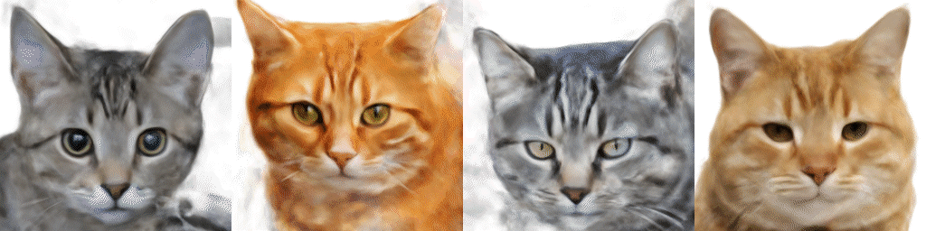
We surprisingly found that fitting only five key points gave accurate enough camera estimates to train a model for cats, dogs, or human faces. This means that given only a single view of your beloved cats Schnitzel, Widget and friends, you can create a new image from any other angle.

Top: example cat images from AFHQ. Bottom: A synthesis of novel 3D views created by LOLNeRF.

Conclusion
We’ve developed a technique that is effective at discovering 3D structure from single 2D images. We see great potential in LOLNeRF for a variety of applications and are currently investigating potential use-cases.

Interpolation of feline identities from linear interpolation of learned latent codes for different examples in AFHQ.

Code Release
We acknowledge the potential for misuse and importance of acting responsibly. To that end, we will only release the code for reproducibility purposes, but will not release any trained generative models.

Acknowledgements
We would like to thank Andrea Tagliasacchi, Kwang Moo Yi, Viral Carpenter, David Fleet, Danica Matthews, Florian Schroff, Hartwig Adam and Dmitry Lagun for continuous help in building this technology.

Source: Google AI Blog


A Multi-Axis Approach for Vision Transformer and MLP Models

Convolutional neural networks have been the dominant machine learning architecture for computer vision since the introduction of AlexNet in 2012. Recently, inspired by the evolution of Transformers in natural language processing, attention mechanisms have been prominently incorporated into vision models. These attention methods boost some parts of the input data while minimizing other parts so that the network can focus on small but important parts of the data. The Vision Transformer (ViT) has created a new landscape of model designs for computer vision that is completely free of convolution. ViT regards image patches as a sequence of words, and applies a Transformer encoder on top. When trained on sufficiently large datasets, ViT demonstrates compelling performance on image recognition.

While convolutions and attention are both sufficient for good performance, neither of them are necessary. For example, MLP-Mixer adopts a simple multi-layer perceptron (MLP) to mix image patches across all the spatial locations, resulting in an all-MLP architecture. It is a competitive alternative to existing state-of-the-art vision models in terms of the trade-off between accuracy and computation required for training and inference. However, both ViT and the MLP models struggle to scale to higher input resolution because the computational complexity increases quadratically with respect to the image size.

Today we present a new multi-axis approach that is simple and effective, improves on the original ViT and MLP models, can better adapt to high-resolution, dense prediction tasks, and can naturally adapt to different input sizes with high flexibility and low complexity. Based on this approach, we have built two backbone models for high-level and low-level vision tasks. We describe the first in “MaxViT: Multi-Axis Vision Transformer”, to be presented in ECCV 2022, and show it significantly improves the state of the art for high-level tasks, such as image classification, object detection, segmentation, quality assessment, and generation. The second, presented in “MAXIM: Multi-Axis MLP for Image Processing” at CVPR 2022, is based on a UNet-like architecture and achieves competitive performance on low-level imaging tasks including denoising, deblurring, dehazing, deraining, and low-light enhancement. To facilitate further research on efficient Transformer and MLP models, we have open-sourced the code and models for both MaxViT and MAXIM.

A demo of image deblurring using MAXIM frame by frame.

Overview
Our new approach is based on multi-axis attention, which decomposes the full-size attention (each pixel attends to all the pixels) used in ViT into two sparse forms — local and (sparse) global. As shown in the figure below, the multi-axis attention contains a sequential stack of block attention and grid attention. The block attention works within non-overlapping windows (small patches in intermediate feature maps) to capture local patterns, while the grid attention works on a sparsely sampled uniform grid for long-range (global) interactions. The window sizes of grid and block attentions can be fully controlled as hyperparameters to ensure a linear computational complexity to the input size.

The proposed multi-axis attention conducts blocked local and dilated global attention sequentially followed by a FFN, with only a linear complexity. The pixels in the same colors are attended together.

Such low-complexity attention can significantly improve its wide applicability to many vision tasks, especially for high-resolution visual predictions, demonstrating greater generality than the original attention used in ViT. We build two backbone instantiations out of this multi-axis attention approach – MaxViT and MAXIM, for high-level and low-level tasks, respectively.

MaxViT
In MaxViT, we first build a single MaxViT block (shown below) by concatenating MBConv (proposed by EfficientNet, V2) with the multi-axis attention. This single block can encode local and global visual information regardless of input resolution. We then simply stack repeated blocks composed of attention and convolutions in a hierarchical architecture (similar to ResNet, CoAtNet), yielding our homogenous MaxViT architecture. Notably, MaxViT is distinguished from previous hierarchical approaches as it can “see” globally throughout the entire network, even in earlier, high-resolution stages, demonstrating stronger model capacity on various tasks.

The meta-architecture of MaxViT.

MAXIM
Our second backbone, MAXIM, is a generic UNet-like architecture tailored for low-level image-to-image prediction tasks. MAXIM explores parallel designs of the local and global approaches using the gated multi-layer perceptron (gMLP) network (patching-mixing MLP with a gating mechanism). Another contribution of MAXIM is the cross-gating block that can be used to apply interactions between two different input signals. This block can serve as an efficient alternative to the cross-attention module as it only employs the cheap gated MLP operators to interact with various inputs without relying on the computationally heavy cross-attention. Moreover, all the proposed components including the gated MLP and cross-gating blocks in MAXIM enjoy linear complexity to image size, making it even more efficient when processing high-resolution pictures.

Results
We demonstrate the effectiveness of MaxViT on a broad range of vision tasks. On image classification, MaxViT achieves state-of-the-art results under various settings: with only ImageNet-1K training, MaxViT attains 86.5% top-1 accuracy; with ImageNet-21K (14M images, 21k classes) pre-training, MaxViT achieves 88.7% top-1 accuracy; and with JFT (300M images, 18k classes) pre-training, our largest model MaxViT-XL achieves a high accuracy of 89.5% with 475M parameters.

Performance comparison of MaxViT with state-of-the-art models on ImageNet-1K. Top: Accuracy vs. FLOPs performance scaling with 224x224 image resolution. Bottom: Accuracy vs. parameters scaling curve under ImageNet-1K fine-tuning setting.

For downstream tasks, MaxViT as a backbone delivers favorable performance on a broad spectrum of tasks. For object detection and segmentation on the COCO dataset, the MaxViT backbone achieves 53.4 AP, outperforming other base-level models while requiring only about 60% the computational cost. For image aesthetics assessment, the MaxViT model advances the state-of-the-art MUSIQ model by 3.5% in terms of linear correlation with human opinion scores. The standalone MaxViT building block also demonstrates effective performance on image generation, achieving better FID and IS scores on the ImageNet-1K unconditional generation task with a significantly lower number of parameters than the state-of-the-art model, HiT.

The UNet-like MAXIM backbone, customized for image processing tasks, has also demonstrated state-of-the-art results on 15 out of 20 tested datasets, including denoising, deblurring, deraining, dehazing, and low-light enhancement, while requiring fewer or comparable number of parameters and FLOPs than competitive models. Images restored by MAXIM show more recovered details with less visual artifacts.

Visual results of MAXIM for image deblurring, deraining, and low-light enhancement.

Summary
Recent works in the last two or so years have shown that ConvNets and Vision Transformers can achieve similar performance. Our work presents a unified design that takes advantage of the best of both worlds — efficient convolution and sparse attention — and demonstrates that a model built on top, namely MaxViT, can achieve state-of-the-art performance on a variety of vision tasks. More importantly, MaxViT scales well to very large data sizes. We also show that an alternative multi-axis design using MLP operators, MAXIM, achieves state-of-the-art performance on a broad range of low-level vision tasks.

Even though we present our models in the context of vision tasks, the proposed multi-axis approach can easily extend to language modeling to capture both local and global dependencies in linear time. Motivated by the work here, we expect that it is worthwhile to study other forms of sparse attention in higher-dimensional or multimodal signals such as videos, point clouds, and vision-language models.

We have open-sourced the code and models of MAXIM and MaxViT to facilitate future research on efficient attention and MLP models.

Acknowledgments
We would like to thank our co-authors: Hossein Talebi, Han Zhang, Feng Yang, Peyman Milanfar, and Alan Bovik. We would also like to acknowledge the valuable discussion and support from Xianzhi Du, Long Zhao, Wuyang Chen, Hanxiao Liu, Zihang Dai, Anurag Arnab, Sungjoon Choi, Junjie Ke, Mauricio Delbracio, Irene Zhu, Innfarn Yoo, Huiwen Chang, and Ce Liu.

Source: Google AI Blog


High-Definition Segmentation in Google Meet

In recent years video conferencing has played an increasingly important role in both work and personal communication for many users. Over the past two years, we have enhanced this experience in Google Meet by introducing privacy-preserving machine learning (ML) powered background features, also known as “virtual green screen”, which allows users to blur their backgrounds or replace them with other images. What is unique about this solution is that it runs directly in the browser without the need to install additional software.

So far, these ML-powered features have relied on CPU inference made possible by leveraging neural network sparsity, a common solution that works across devices, from entry level computers to high-end workstations. This enables our features to reach the widest audience. However, mid-tier and high-end devices often have powerful GPUs that remain untapped for ML inference, and existing functionality allows web browsers to access GPUs via shaders (WebGL).

With the latest update to Google Meet, we are now harnessing the power of GPUs to significantly improve the fidelity and performance of these background effects. As we detail in “Efficient Heterogeneous Video Segmentation at the Edge”, these advances are powered by two major components: 1) a novel real-time video segmentation model and 2) a new, highly efficient approach for in-browser ML acceleration using WebGL. We leverage this capability to develop fast ML inference via fragment shaders. This combination results in substantial gains in accuracy and latency, leading to crisper foreground boundaries.

CPU segmentation vs. HD segmentation in Meet.

Moving Towards Higher Quality Video Segmentation Models
To predict finer details, our new segmentation model now operates on high definition (HD) input images, rather than lower-resolution images, effectively doubling the resolution over the previous model. To accommodate this, the model must be of higher capacity to extract features with sufficient detail. Roughly speaking, doubling the input resolution quadruples the computation cost during inference.

Inference of high-resolution models using the CPU is not feasible for many devices. The CPU may have a few high-performance cores that enable it to execute arbitrary complex code efficiently, but it is limited in its ability for the parallel computation required for HD segmentation. In contrast, GPUs have many, relatively low-performance cores coupled with a wide memory interface, making them uniquely suitable for high-resolution convolutional models. Therefore, for mid-tier and high-end devices, we adopt a significantly faster pure GPU pipeline, which is integrated using WebGL.

This change inspired us to revisit some of the prior design decisions for the model architecture.

  • Backbone: We compared several widely-used backbones for on-device networks and found EfficientNet-Lite to be a better fit for the GPU because it removes the squeeze-and-excitation block, a component that is inefficient on WebGL (more below).
  • Decoder: We switched to a multi-layer perceptron (MLP) decoder consisting of 1x1 convolutions instead of using simple bilinear upsampling or the more expensive squeeze-and-excitation blocks. MLP has been successfully adopted in other segmentation architectures, like DeepLab and PointRend, and is efficient to compute on both CPU and GPU.
  • Model size: With our new WebGL inference and the GPU-friendly model architecture, we were able to afford a larger model without sacrificing the real-time frame rate necessary for smooth video segmentation. We explored the width and the depth parameters using a neural architecture search.
HD segmentation model architecture.

In aggregate, these changes substantially improve the mean Intersection over Union (IoU) metric by 3%, resulting in less uncertainty and crisper boundaries around hair and fingers.

We have also released the accompanying model card for this segmentation model, which details our fairness evaluations. Our analysis shows that the model is consistent in its performance across the various regions, skin-tones, and genders, with only small deviations in IoU metrics.

Model     Resolution     Inference     IoU     Latency (ms)
CPU segmenter     256×144     Wasm SIMD     94.0%     8.7
GPU segmenter     512×288     WebGL     96.9%     4.3
Comparison of the previous segmentation model vs. the new HD segmentation model on a Macbook Pro (2018).

Accelerating Web ML with WebGL
One common challenge for web-based inference is that web technologies can incur a performance penalty when compared to apps running natively on-device. For GPUs, this penalty is substantial, only achieving around 25% of native OpenGL performance. This is because WebGL, the current GPU standard for Web-based inference, was primarily designed for image rendering, not arbitrary ML workloads. In particular, WebGL does not include compute shaders, which allow for general purpose computation and enable ML workloads in mobile and native apps.

To overcome this challenge, we accelerated low-level neural network kernels with fragment shaders that typically compute the output properties of a pixel like color and depth, and then applied novel optimizations inspired by the graphics community. As ML workloads on GPUs are often bound by memory bandwidth rather than compute, we focused on rendering techniques that would improve the memory access, such as Multiple Render Targets (MRT).

MRT is a feature in modern GPUs that allows rendering images to multiple output textures (OpenGL objects that represent images) at once. While MRT was originally designed to support advanced graphics rendering such as deferred shading, we found that we could leverage this feature to drastically reduce the memory bandwidth usage of our fragment shader implementations for critical operations, like convolutions and fully connected layers. We do so by treating intermediate tensors as multiple OpenGL textures.

In the figure below, we show an example of intermediate tensors having four underlying GL textures each. With MRT, the number of GPU threads, and thus effectively the number of memory requests for weights, is reduced by a factor of four and saves memory bandwidth usage. Although this introduces considerable complexities in the code, it helps us reach over 90% of native OpenGL performance, closing the gap with native applications.

Left: A classic implementation of Conv2D with 1-to-1 correspondence of tensor and an OpenGL texture. Red, yellow, green, and blue boxes denote different locations in a single texture each for intermediate tensor A and B. Right: Our implementation of Conv2D with MRT where intermediate tensors A and B are realized with a set of 4 GL textures each, depicted as red, yellow, green, and blue boxes. Note that this reduces the request count for weights by 4x.

Conclusion
We have made rapid strides in improving the quality of real-time segmentation models by leveraging the GPU on mid-tier and high-end devices for use with Google Meet. We look forward to the possibilities that will be enabled by upcoming technologies like WebGPU, which bring compute shaders to the web. Beyond GPU inference, we're also working on improving the segmentation quality for lower powered devices with quantized inference via XNNPACK WebAssembly.

Acknowledgements
Special thanks to those on the Meet team and others who worked on this project, in particular Sebastian Jansson, Sami Kalliomäki, Rikard Lundmark, Stephan Reiter, Fabian Bergmark, Ben Wagner, Stefan Holmer, Dan Gunnarsson, Stéphane Hulaud, and to all our team members who made this possible: Siargey Pisarchyk, Raman Sarokin, Artsiom Ablavatski, Jamie Lin, Tyler Mullen, Gregory Karpiak, Andrei Kulik, Karthik Raveendran, Trent Tolley, and Matthias Grundmann.

Source: Google AI Blog


UVQ: Measuring YouTube’s Perceptual Video Quality

Online video sharing platforms, like YouTube, need to understand perceptual video quality (i.e., a user's subjective perception of video quality) in order to better optimize and improve user experience. Video quality assessment (VQA) attempts to build a bridge between video signals and perceptual quality by using objective mathematical models to approximate the subjective opinions of users. Traditional video quality metrics, like peak signal-to-noise ratio (PSNR) and Video Multi-Method Assessment Fusion (VMAF), are reference-based and focus on the relative difference between the target and reference videos. Such metrics, which work best on professionally generated content (e.g., movies), assume the reference video is of pristine quality and that one can induce the target video's absolute quality from the relative difference.

However, the majority of the videos that are uploaded on YouTube are user-generated content (UGC), which bring new challenges due to their remarkably high variability in video content and original quality. Most UGC uploads are non-pristine and the same amount of relative difference could imply very different perceptual quality impacts. For example, people tend to be less sensitive to the distortions of poor quality uploads than of high quality uploads. Thus, reference-based quality scores become inaccurate and inconsistent when used for UGC cases. Additionally, despite the high volume of UGC, there are currently limited UGC video quality assessment (UGC-VQA) datasets with quality labels. Existing UGC-VQA datasets are either small in size (e.g., LIVE-Qualcomm has 208 samples captured from 54 unique scenes), compared with datasets with millions of samples for classification and recognition (e.g., ImageNet and YouTube-8M), or don’t have enough content variability (sampling without considering content information, like LIVE-VQC and KoNViD-1k).

In "Rich Features for Perceptual Quality Assessment of UGC Videos", published at CVPR 2021, we describe how we attempt to solve the UGC quality assessment problem by building a Universal Video Quality (UVQ) model that resembles a subjective quality assessment. The UVQ model uses subnetworks to analyze UGC quality from high-level semantic information to low-level pixel distortions, and provides a reliable quality score with rationale (leveraging comprehensive and interpretable quality labels). Moreover, to advance UGC-VQA and compression research, we enhance the open-sourced YouTube-UGC dataset, which contains 1.5K representative UGC samples from millions of UGC videos (distributed under the Creative Commons license) on YouTube. The updated dataset contains ground-truth labels for both original videos and corresponding transcoded versions, enabling us to better understand the relationship between video content and its perceptual quality.

Subjective Video Quality Assessment
To understand perceptual video quality, we leverage an internal crowd-sourcing platform to collect mean opinion scores (MOS) with a scale of 1–5, where 1 is the lowest quality and 5 is the highest quality, for no-reference use cases. We collect ground-truth labels from the YouTube-UGC dataset and categorize UGC factors that affect quality perception into three high-level categories: (1) content, (2) distortions, and (3) compression. For example, a video with no meaningful content won't receive a high quality MOS. Also, distortions introduced during the video production phase and video compression artifacts introduced by third-party platforms, e.g., transcoding or transmission, will degrade the overall quality.

MOS= 2.052 MOS= 4.457
Left: A video with no meaningful content won't receive a high quality MOS. Right: A video displaying intense sports shows a higher MOS.
MOS= 1.242 MOS= 4.522
Left: A blurry gaming video gets a very low quality MOS. Right: A video with professional rendering (high contrast and sharp edges, usually introduced in the video production phase) shows a high quality MOS.
MOS= 2.372 MOS= 4.646
Left: A heavily compressed video receives a low quality MOS. Right: a video without compression artifacts shows a high quality MOS.

We demonstrate that the left gaming video in the second row of the figure above has the lowest MOS (1.2), even lower than the video with no meaningful content. A possible explanation is that viewers may have higher video quality expectations for videos that have a clear narrative structure, like gaming videos, and the blur artifacts significantly reduce the perceptual quality of the video.

UVQ Model Framework
A common method for evaluating video quality is to design sophisticated features, and then map these features to a MOS. However, designing useful handcrafted features is difficult and time-consuming, even for domain experts. Also, the most useful existing handcrafted features were summarized from limited samples, which may not perform well on broader UGC cases. In contrast, machine learning is becoming more prominent in UGC-VQA because it can automatically learn features from large-scale samples.

A straightforward approach is to train a model from scratch on existing UGC quality datasets. However, this may not be feasible as there are limited quality UGC datasets. To overcome this limitation, we apply a self-supervised learning step to the UVQ model during training. This self-supervised step enables us to learn comprehensive quality-related features, without ground-truth MOS, from millions of raw videos.

Following the quality-related categories summarized from the subjective VQA, we develop the UVQ model with four novel subnetworks. The first three subnetworks, which we call ContentNet, DistortionNet and CompressionNet, are used to extract quality features (i.e., content, distortion and compression), and the fourth subnetwork, called AggregationNet, maps the extracted features to generate a single quality score. ContentNet is trained in a supervised learning fashion with UGC-specific content labels that are generated by the YouTube-8M model. DistortionNet is trained to detect common distortions, e.g., Gaussian blur and white noise of the original frame. CompressionNet focuses on video compression artifacts, whose training data are videos compressed with different bitrates. CompressionNet is trained using two compressed variants of the same content that are fed into the model to predict corresponding compression levels (with a higher score for more noticeable compression artifacts), with the implicit assumption that the higher bitrate version has a lower compression level.

The ContentNet, DistortionNet and CompressionNet subnetworks are trained on large-scale samples without ground-truth quality scores. Since video resolution is also an important quality factor, the resolution-sensitive subnetworks (CompressionNet and DistortionNet) are patch-based (i.e., each input frame is divided into multiple disjointed patches that are processed separately), which makes it possible to capture all detail on native resolution without downscaling. The three subnetworks extract quality features that are then concatenated by the fourth subnetwork, AggregationNet, to predict quality scores with domain ground-truth MOS from YouTube-UGC.

The UVQ training framework.

Analyzing Video Quality with UVQ
After building the UVQ model, we use it to analyze the video quality of samples pulled from YouTube-UGC and demonstrate that its subnetworks can provide a single quality score along with high-level quality indicators that can help us understand quality issues. For example, DistortionNet detects multiple visual artifacts, e.g., jitter and lens blur, for the middle video below, and CompressionNet detects that the bottom video has been heavily compressed.

ContentNet assigns content labels with corresponding probabilities in parentheses, i.e., car (0.58), vehicle (0.42), sports car (0.32), motorsports (0.18), racing (0.11).
DistortionNet detects and categorizes multiple visual distortions with corresponding probabilities in parentheses, i.e., jitter (0.112), color quantization (0.111), lens blur (0.108), denoise (0.107).
CompressionNet detects a high compression level of 0.892 for the video above.

Additionally, UVQ can provide patch-based feedback to locate quality issues. Below, UVQ reports that the quality of the first patch (patch at time t = 1) is good with a low compression level. However, the model identifies heavy compression artifacts in the next patch (patch at time t = 2).

Patch at time t = 1 Patch at time t = 2
Compression level = 0.000 Compression level = 0.904
UVQ detects a sudden quality degradation (high compression level) for a local patch.

In practice, UVQ can generate a video diagnostic report that includes a content description (e.g., strategy video game), distortion analysis (e.g., the video is blurry or pixelated) and compression level (e.g., low or high compression). Below, UVQ reports that the content quality, looking at individual features, is good, but the compression and distortion quality is low. When combining all three features, the overall quality is medium-low. We see that these findings are close to the rationale summarized by internal user experts, demonstrating that UVQ can reason through quality assessments, while providing a single quality score.

UVQ diagnostic report. ContentNet (CT): Video game, strategy video game, World of Warcraft, etc. DistortionNet (DT): multiplicative noise, Gaussian blur, color saturation, pixelate, etc. CompressionNet (CP): 0.559 (medium-high compression). Predicted quality score in [1, 5]: (CT, DT, CP) = (3.901, 3.216, 3.151), (CT+DT+CP) = 3.149 (medium-low quality).

Conclusion
We present the UVQ model, which generates a report with quality scores and insights that can be used to interpret UGC video perceptual quality. UVQ learns comprehensive quality related features from millions of UGC videos and provides a consistent view of quality interpretation for both no-reference and reference cases. To learn more, read our paper or visit our website to see YT-UGC videos and their subjective quality data. We also hope that the enhanced YouTube-UGC dataset enables more research in this space.

Acknowledgements
This work was possible through a collaboration spanning several Google teams. Key contributors include: Balu Adsumilli, Neil Birkbeck, Joong Gon Yim from YouTube and Junjie Ke, Hossein Talebi, Peyman Milanfar from Google Research. Thanks to Ross Wolf, Jayaprasanna Jayaraman, Carena Church, and Jessie Lin for their contributions.

Source: Google AI Blog


Efficient Video-Text Learning with Iterative Co-tokenization

Video is an ubiquitous source of media content that touches on many aspects of people’s day-to-day lives. Increasingly, real-world video applications, such as video captioning, video content analysis, and video question-answering (VideoQA), rely on models that can connect video content with text or natural language. VideoQA is particularly challenging, however, as it requires grasping both semantic information, such as objects in a scene, as well as temporal information, e.g., how things move and interact, both of which must be taken in the context of a natural-language question that holds specific intent. In addition, because videos have many frames, processing all of them to learn spatio-temporal information can be computationally expensive. Nonetheless, understanding all this information enables models to answer complex questions — for example, in the video below, a question about the second ingredient poured in the bowl requires identifying objects (the ingredients), actions (pouring), and temporal ordering (second).

An example input question for the VideoQA task “What is the second ingredient poured into the bowl?” which requires deeper understanding of both the visual and text inputs. The video is an example from the 50 Salads dataset, used under the Creative Commons license.

To address this, in “Video Question Answering with Iterative Video-Text Co-Tokenization”, we introduce a new approach to video-text learning called iterative co-tokenization, which is able to efficiently fuse spatial, temporal and language information for VideoQA. This approach is multi-stream, processing different scale videos with independent backbone models for each to produce video representations that capture different features, e.g., those of high spatial resolution or long temporal durations. The model then applies the co-tokenization module to learn efficient representations from fusing the video streams with the text. This model is highly efficient, using only 67 giga-FLOPs (GFLOPs), which is at least 50% fewer than previous approaches, while giving better performance than alternative state-of-the-art models.

Video-Text Iterative Co-tokenization
The main goal of the model is to produce features from both videos and text (i.e., the user question), jointly allowing their corresponding inputs to interact. A second goal is to do so in an efficient manner, which is highly important for videos since they contain tens to hundreds of frames as input.

The model learns to tokenize the joint video-language inputs into a smaller set of tokens that jointly and efficiently represent both modalities. When tokenizing, we use both modalities to produce a joint compact representation, which is fed to a transformer layer to produce the next level representation. A challenge here, which is also typical in cross-modal learning, is that often the video frame does not correspond directly to the associated text. We address this by adding two learnable linear layers which unify the visual and text feature dimensions before tokenization. This way we enable both video and text to condition how video tokens are learned.

Moreover, a single tokenization step does not allow for further interaction between the two modalities. For that, we use this new feature representation to interact with the video input features and produce another set of tokenized features, which are then fed into the next transformer layer. This iterative process allows the creation of new features, or tokens, which represent a continual refinement of the joint representation from both modalities. At the last step the features are input to a decoder that generates the text output.

As customarily done for VideoQA, we pre-train the model before fine-tuning it on the individual VideoQA datasets. In this work we use the videos automatically annotated with text based on speech recognition, using the HowTo100M dataset instead of pre-training on a large VideoQA dataset. This weaker pre-training data still enables our model to learn video-text features.

Visualization of the video-text iterative co-tokenization approach. Multi-stream video inputs, which are versions of the same video input (e.g., a high resolution, low frame-rate video and a low resolution, high frame-rate video), are efficiently fused together with the text input to produce a text-based answer by the decoder. Instead of processing the inputs directly, the video-text iterative co-tokenization model learns a reduced number of useful tokens from the fused video-language inputs. This process is done iteratively, allowing the current feature tokenization to affect the selection of tokens at the next iteration, thus refining the selection.

Efficient Video Question-Answering
We apply the video-language iterative co-tokenization algorithm to three main VideoQA benchmarks, MSRVTT-QA, MSVD-QA and IVQA, and demonstrate that this approach achieves better results than other state-of-the-art models, while having a modest size. Furthermore, iterative co-tokenization learning yields significant compute savings for video-text learning tasks. The method uses only 67 giga-FLOPs (GFLOPS), which is one sixth the 360 GFLOPS needed when using the popular 3D-ResNet video model jointly with text and is more than twice as efficient as the X3D model. This is all the while producing highly accurate results, outperforming state-of-the-art methods.

Comparison of our iterative co-tokenization approach to previous methods such as MERLOT and VQA-T, as well as, baselines using single ResNet-3D or X3D-XL.

Multi-stream Video Inputs
For VideoQA, or any of a number of other tasks that involve video inputs, we find that multi-stream input is important to more accurately answer questions about both spatial and temporal relationships. Our approach utilizes three video streams at different resolutions and frame-rates: a low-resolution high frame-rate, input video stream (with 32 frames-per-second and spatial resolution 64x64, which we denote as 32x64x64); a high-resolution, low frame-rate video (8x224x224); and one in-between (16x112x112). Despite the apparently more voluminous information to process with three streams, we obtain very efficient models due to the iterative co-tokenization approach. At the same time these additional streams allow extraction of the most pertinent information. For example, as shown in the figure below, questions related to a specific activity in time will produce higher activations in the smaller resolution but high frame-rate video input, whereas questions related to the general activity can be answered from the high resolution input with very few frames. Another benefit of this algorithm is that the tokenization changes depending on the questions asked.

Visualization of the attention maps learned per layer during the video-text co-tokenization. The attention maps differ depending on the question asked for the same video. For example, if the question is related to the general activity (e.g., surfing in the figure above), then the attention maps of the higher resolution low frame-rate inputs are more active and seem to consider more global information. Whereas if the question is more specific, e.g., asking about what happens after an event, the feature maps are more localized and tend to be active in the high frame-rate video input. Furthermore, we see that the low-resolution, high-frame rate video inputs provide more information related to activities in the video.

Conclusion
We present a new approach to video-language learning that focuses on joint learning across video-text modalities. We address the important and challenging task of video question-answering. Our approach is both highly efficient and accurate, outperforming current state-of-the-art models, despite being more efficient. Our approach results in modest model sizes and can gain further improvements with larger models and data. We hope this work provokes more research in vision-language learning to enable more seamless interaction with vision-based media.

Acknowledgements
This work is conducted by AJ Pierviovanni, Kairo Morton, Weicheng Kuo, Michael Ryoo and Anelia Angelova. We thank our collaborators in this research, and Soravit Changpinyo for valuable comments and suggestions, and Claire Cui for suggestions and support. We also thank Tom Small for visualizations.

Source: Google AI Blog


Introducing the Google Universal Image Embedding Challenge

Computer vision models see daily application for a wide variety of tasks, ranging from object recognition to image-based 3D object reconstruction. One challenging type of computer vision problem is instance-level recognition (ILR) — given an image of an object, the task is to not only determine the generic category of an object (e.g., an arch), but also the specific instance of the object (”Arc de Triomphe de l'Étoile, Paris, France”).

Previously, ILR was tackled using deep learning approaches. First, a large set of images was collected. Then a deep model was trained to embed each image into a high-dimensional space where similar images have similar representations. Finally, the representation was used to solve the ILR tasks related to classification (e.g., with a shallow classifier trained on top of the embedding) or retrieval (e.g., with a nearest neighbor search in the embedding space).

Since there are many different object domains in the world, e.g., landmarks, products, or artworks, capturing all of them in a single dataset and training a model that can distinguish between them is quite a challenging task. To decrease the complexity of the problem to a manageable level, the focus of research so far has been to solve ILR for a single domain at a time. To advance the research in this area, we hosted multiple Kaggle competitions focused on the recognition and retrieval of landmark images. In 2020, Amazon joined the effort and we moved beyond the landmark domain and expanded to the domains of artwork and product instance recognition. The next step is to generalize the ILR task to multiple domains.

To this end, we’re excited to announce the Google Universal Image Embedding Challenge, hosted by Kaggle in collaboration with Google Research and Google Lens. In this challenge, we ask participants to build a single universal image embedding model capable of representing objects from multiple domains at the instance level. We believe that this is the key for real-world visual search applications, such as augmenting cultural exhibits in a museum, organizing photo collections, visual commerce and more.

Images1 of object instances coming from multiple domains, which are represented in our dataset: apparel and accessories, packaged goods, furniture and home goods, toys, cars, landmarks, storefronts, dishes, artwork, memes and illustrations.

Degrees of Variation in Different Domains
To represent objects from a large number of domains, we require one model to learn many domain-specific subtasks (e.g., filtering different kinds of noise or focusing on a specific detail), which can only be learned from a semantically and visually diverse collection of images. Addressing each degree of variation proposes a new challenge for both image collection and model training.

The first sort of variation comes from the fact that while some domains contain unique objects in the world (landmarks, artwork, etc.), others contain objects that may have many copies (clothing, furniture, packaged goods, food, etc.). Because a landmark is always placed at the same location, the surrounding context may be useful for recognition. In contrast, a product, say a phone, even of a specific model and color, may have millions of physical instances and thus appear in many surrounding contexts.

Another challenge comes from the fact that a single object may appear different depending on the point of view, lighting conditions, occlusion or deformations (e.g., a dress worn on a person may look very different than on a hanger). In order for a model to learn invariance to all of these visual modes, all of them should be captured by the training data.

Additionally, similarities between objects differ across domains. For example, in order for a representation to be useful in the product domain, it must be able to distinguish very fine-grained details between similarly looking products belonging to two different brands. In the domain of food, however, the same dish (e.g., spaghetti bolognese) cooked by two chefs may look quite different, but the ability of the model to distinguish spaghetti bolognese from other dishes may be sufficient for the model to be useful. Additionally, a vision model of high quality should assign similar representations to more visually similar renditions of a dish.

Domain    Landmark    Apparel
Image      
Instance Name    Empire State Building2    Cycling jerseys with Android logo3

Which physical objects belong to the instance class?    Single instance in the world    Many physical instances; may differ in size or pattern (e.g., a patterned cloth cut differently)

What are the possible views of the object?    Appearance variation only based on capture conditions (e.g., illumination or viewpoint); limited number of common external views; possibility of many internal views    Deformable appearance (e.g., worn or not); limited number of common views: front, back, side

What are the surroundings and are they useful for recognition?    Surrounding context does not vary much other than daily and yearly cycles; may be useful for verifying the object of interest    Surrounding context can change dramatically due to difference in environment, additional pieces of clothing, or accessories partially occluding clothing of interest (e.g., a jacket or a scarf)

What may be tricky cases that do not belong to the instance class?    Replicas of landmarks (e.g., Eiffel Tower in Las Vegas), souvenirs    Same piece of apparel of different material or different color; visually very similar pieces with a small distinguishing detail (e.g., a small brand logo); different pieces of apparel worn by the same model
Variation among domains for landmark and apparel examples.

Learning Multi-domain Representations
After a collection of images covering a variety of domains is created, the next challenge is to train a single, universal model. Some features and tasks, such as representing color, are useful across many domains, and thus adding training data from any domain will likely help the model improve at distinguishing colors. Other features may be more specific to selected domains, thus adding more training data from other domains may deteriorate the model’s performance. For example, while for 2D artwork it may be very useful for the model to learn to find near duplicates, this may deteriorate the performance on clothing, where deformed and occluded instances need to be recognized.

The large variety of possible input objects and tasks that need to be learned require novel approaches for selecting, augmenting, cleaning and weighing the training data. New approaches for model training and tuning, and even novel architectures may be required.

Universal Image Embedding Challenge
To help motivate the research community to address these challenges, we are hosting the Google Universal Image Embedding Challenge. The challenge was launched on Kaggle in July and will be open until October, with cash prizes totaling $50k. The winning teams will be invited to present their methods at the Instance-Level Recognition workshop at ECCV 2022.

Participants will be evaluated on a retrieval task on a dataset of ~5,000 test query images and ~200,000 index images, from which similar images are retrieved. In contrast to ImageNet, which includes categorical labels, the images in this dataset are labeled at the instance level.

The evaluation data for the challenge is composed of images from the following domains: apparel and accessories, packaged goods, furniture and home goods, toys, cars, landmarks, storefronts, dishes, artwork, memes and illustrations.

Distribution of domains of query images.

We invite researchers and machine learning enthusiasts to participate in the Google Universal Image Embedding Challenge and join the Instance-Level Recognition workshop at ECCV 2022. We hope the challenge and the workshop will advance state-of-the-art techniques on multi-domain representations.

Acknowledgement
The core contributors to this project are Andre Araujo, Boris Bluntschli, Bingyi Cao, Kaifeng Chen, Mário Lipovský, Grzegorz Makosa, Mojtaba Seyedhosseini and Pelin Dogan Schönberger. We would like to thank Sohier Dane, Will Cukierski and Maggie Demkin for their help organizing the Kaggle challenge, as well as our ECCV workshop co-organizers Tobias Weyand, Bohyung Han, Shih-Fu Chang, Ondrej Chum, Torsten Sattler, Giorgos Tolias, Xu Zhang, Noa Garcia, Guangxing Han, Pradeep Natarajan and Sanqiang Zhao. Furthermore we are thankful to Igor Bonaci, Tom Duerig, Vittorio Ferrari, Victor Gomes, Futang Peng and Howard Zhou who gave us feedback, ideas and support at various points of this project.


1 Image credits: Chris Schrier, CC-BY; Petri Krohn, GNU Free Documentation License; Drazen Nesic, CC0; Marco Verch Professional Photographer, CCBY; Grendelkhan, CCBY; Bobby Mikul, CC0; Vincent Van Gogh, CC0; pxhere.com, CC0; Smart Home Perfected, CC-BY.  
2 Image credit: Bobby Mikul, CC0.  
3 Image credit: Chris Schrier, CC-BY.  

Source: Google AI Blog


Building Efficient Multiple Visual Domain Models with Multi-path Neural Architecture Search

Deep learning models for visual tasks (e.g., image classification) are usually trained end-to-end with data from a single visual domain (e.g., natural images or computer generated images). Typically, an application that completes visual tasks for multiple domains would need to build multiple models for each individual domain, train them independently (meaning no data is shared between domains), and then at inference time each model would process domain-specific input data. However, early layers between these models generate similar features, even for different domains, so it can be more efficient — decreasing latency and power consumption, lower memory overhead to store parameters of each model — to jointly train multiple domains, an approach referred to as multi-domain learning (MDL). Moreover, an MDL model can also outperform single domain models due to positive knowledge transfer, which is when additional training on one domain actually improves performance for another. The opposite, negative knowledge transfer, can also occur, depending on the approach and specific combination of domains involved. While previous work on MDL has proven the effectiveness of jointly learning tasks across multiple domains, it involved a hand-crafted model architecture that is inefficient to apply to other work.

In “Multi-path Neural Networks for On-device Multi-domain Visual Classification”, we propose a general MDL model that can: 1) achieve high accuracy efficiently (keeping the number of parameters and FLOPS low), 2) learn to enhance positive knowledge transfer while mitigating negative transfer, and 3) effectively optimize the joint model while handling various domain-specific difficulties. As such, we propose a multi-path neural architecture search (MPNAS) approach to build a unified model with heterogeneous network architecture for multiple domains. MPNAS extends the efficient neural architecture search (NAS) approach from single path search to multi-path search by finding an optimal path for each domain jointly. Also, we introduce a new loss function, called adaptive balanced domain prioritization (ABDP) that adapts to domain-specific difficulties to help train the model efficiently. The resulting MPNAS approach is efficient and scalable; the resulting model maintains performance while reducing the model size and FLOPS by 78% and 32%, respectively, compared to a single-domain approach.

Multi-Path Neural Architecture Search
To encourage positive knowledge transfer and avoid negative transfer, traditional solutions build an MDL model so that domains share most of the layers that learn the shared features across domains (called feature extraction), then have a few domain-specific layers on top. However, such a homogenous approach to feature extraction cannot handle domains with significantly different features (e.g., objects in natural images and art paintings). On the other hand, handcrafting a unified heterogeneous architecture for each MDL model is time-consuming and requires domain-specific knowledge.

NAS is a powerful paradigm for automatically designing deep learning architectures. It defines a search space, made up of various potential building blocks that could be part of the final model. The search algorithm finds the best candidate architecture from the search space that optimizes the model objectives, e.g., classification accuracy. Recent NAS approaches (e.g., TuNAS) have meaningfully improved search efficiency by using end-to-end path sampling, which enables us to scale NAS from single domains to MDL.

Inspired by TuNAS, MPNAS builds the MDL model architecture in two stages: search and training. In the search stage, to find an optimal path for each domain jointly, MPNAS creates an individual reinforcement learning (RL) controller for each domain, which samples an end-to-end path (from input layer to output layer) from the supernetwork (i.e., the superset of all the possible subnetworks between the candidate nodes defined by the search space). Over multiple iterations, all the RL controllers update the path to optimize the RL rewards across all domains. At the end of the search stage, we obtain a subnetwork for each domain. Finally, all the subnetworks are combined to build a heterogeneous architecture for the MDL model, shown below.

Since the subnetwork for each domain is searched independently, the building block in each layer can be shared by multiple domains (i.e., dark gray nodes), used by a single domain (i.e., light gray nodes), or not used by any subnetwork (i.e., dotted nodes). The path for each domain can also skip any layer during search. Given the subnetwork can freely select which blocks to use along the path in a way that optimizes performance (rather than, e.g., arbitrarily designating which layers are homogenous and which are domain-specific), the output network is both heterogeneous and efficient.

Example architecture searched by MPNAS. Dashed paths represent all the possible subnetworks. Solid paths represent the selected subnetworks for each domain (highlighted in different colors). Nodes in each layer represent the candidate building blocks defined by the search space.

The figure below demonstrates the searched architecture of two visual domains among the ten domains of the Visual Domain Decathlon challenge. One can see that the subnetwork of these two highly related domains (one red, the other green) share a majority of building blocks from their overlapping paths, but there are still some differences.

Architecture blocks of two domains (ImageNet and Describable Textures) among the ten domains of the Visual Domain Decathlon challenge. Red and green path represents the subnetwork of ImageNet and Describable Textures, respectively. Dark pink nodes represent the blocks shared by multiple domains. Light pink nodes represent the blocks used by each path. The model is built based on MobileNet V3-like search space. The “dwb” block in the figure represents the dwbottleneck block. The “zero” block in the figure indicates the subnetwork skips that block.

Below we show the path similarity between domains among the ten domains of the Visual Domain Decathlon challenge. The similarity is measured by the Jaccard similarity score between the subnetworks of each domain, where higher means the paths are more similar. As one might expect, domains that are more similar share more nodes in the paths generated by MPNAS, which is also a signal of strong positive knowledge transfer. For example, the paths for similar domains (like ImageNet, CIFAR-100, and VGG Flower, which all include objects in natural images) have high scores, while the paths for dissimilar domains (like Daimler Pedestrian Classification and UCF101 Dynamic Images, which include pedestrians in grayscale images and human activity in natural color images, respectively) have low scores.

Confusion matrix for the Jaccard similarity score between the paths for the ten domains. Score value ranges from 0 to 1. A greater value indicates two paths share more nodes.

Training a Heterogeneous Multi-domain Model
In the second stage, the model resulting from MPNAS is trained from scratch for all domains. For this to work, it is necessary to define a unified objective function for all the domains. To successfully handle a large variety of domains, we designed an algorithm that adapts throughout the learning process such that losses are balanced across domains, called adaptive balanced domain prioritization (ABDP).

Below we show the accuracy, model size, and FLOPS of the model trained in different settings. We compare MPNAS to three other approaches:

  • Domain independent NAS: Searching and training a model for each domain separately.
  • Single path multi-head: Using a pre-trained model as a shared backbone for all domains with separated classification heads for each domain.
  • Multi-head NAS: Searching a unified backbone architecture for all domains with separated classification heads for each domain.

From the results, we can observe that domain independent NAS requires building a bundle of models for each domain, resulting in a large model size. Although single path multi-head and multi-head NAS can reduce the model size and FLOPS significantly, forcing the domains to share the same backbone introduces negative knowledge transfer, decreasing overall accuracy.

Model   Number of parameters ratio     GFLOPS     Average Top-1 accuracy  
Domain independent NAS     5.7x 1.08 69.9
Single path multi-head 1.0x 0.09 35.2
Multi-head NAS 0.7x 0.04 45.2
MPNAS 1.3x 0.73 71.8
Number of parameters, gigaFLOPS, and Top-1 accuracy (%) of MDL models on the Visual Decathlon dataset. All methods are built based on the MobileNetV3-like search space.

MPNAS can build a small and efficient model while still maintaining high overall accuracy. The average accuracy of MPNAS is even 1.9% higher than the domain independent NAS approach since the model enables positive knowledge transfer. The figure below compares per domain top-1 accuracy of these approaches.

Top-1 accuracy of each Visual Decathlon domain.

Our evaluation shows that top-1 accuracy is improved from 69.96% to 71.78% (delta: +1.81%) by using ABDP as part of the search and training stages.

Top-1 accuracy for each Visual Decathlon domain trained by MPNAS with and without ABDP.

Future Work
We find MPNAS is an efficient solution to build a heterogeneous network to address the data imbalance, domain diversity, negative transfer, domain scalability, and large search space of possible parameter sharing strategies in MDL. By using a MobileNet-like search space, the resulting model is also mobile friendly. We are continuing to extend MPNAS for multi-task learning for tasks that are not compatible with existing search algorithms and hope others might use MPNAS to build a unified multi-domain model.

Acknowledgements
This work is made possible through a collaboration spanning several teams across Google. We’d like to acknowledge contributions from Junjie Ke, Joshua Greaves, Grace Chu, Ramin Mehran, Gabriel Bender, Xuhui Jia, Brendan Jou, Yukun Zhu, Luciano Sbaiz, Alec Go, Andrew Howard, Jeff Gilbert, Peyman Milanfar, and Ming-Tsuan Yang.

Source: Google AI Blog