As a working father with two kids who grew up in the digital era — and as a professional working in online safety outreach and engagement for the last 17 years — I’ve se…
The Dev channel has been updated to 118.0.5979.0 for Mac and Linux, 118.0.5979.0 /.2 for Windows.
A partial list of changes is available in the Git log. Interested in switching release channels? Find out how. If you find a new issue, please let us know by filing a bug. The community help forum is also a great place to reach out for help or learn about common issues.
Posted by Stephan Rasp, Research Scientist, and Carla Bromberg, Program Lead, Google Research
In 1950, weather forecasting started its digital revolution when researchers used the first programmable, general-purpose computer ENIAC to solve mathematical equations describing how weather evolves. In the more than 70 years since, continuous advancements in computing power and improvements to the model formulations have led to steady gains in weather forecast skill: a 7-day forecast today is about as accurate as a 5-day forecast in 2000 and a 3-day forecast in 1980. While improving forecast accuracy at the pace of approximately one day per decade may not seem like a big deal, every day improved is important in far reaching use cases, such as for logistics planning, disaster management, agriculture and energy production. This “quiet” revolution has been tremendously valuable to society, saving lives and providing economic value across many sectors.
Now we are seeing the start of yet another revolution in weather forecasting, this time fueled by advances in machine learning (ML). Rather than hard-coding approximations of the physical equations, the idea is to have algorithms learn how weather evolves from looking at large volumes of past weather data. Early attempts at doing so go back to 2018 but the pace picked up considerably in the last two years when several large ML models demonstrated weather forecasting skill comparable to the best physics-based models. Google’s MetNet [1, 2], for instance, demonstrated state-of-the-art capabilities for forecasting regional weather one day ahead. For global prediction, Google DeepMind created GraphCast, a graph neural network to make 10 day predictions at a horizontal resolution of 25 km, competitive with the best physics-based models in many skill metrics.
Apart from potentially providing more accurate forecasts, one key advantage of such ML methods is that, once trained, they can create forecasts in a matter of minutes on inexpensive hardware. In contrast, traditional weather forecasts require large super-computers that run for hours every day. Clearly, ML represents a tremendous opportunity for the weather forecasting community. This has also been recognized by leading weather forecasting centers, such as the European Centre for Medium-Range Weather Forecasts’ (ECMWF) machine learning roadmap or the National Oceanic and Atmospheric Administration’s (NOAA) artificial intelligence strategy.
To ensure that ML models are trusted and optimized for the right goal, forecast evaluation is crucial. Evaluating weather forecasts isn’t straightforward, however, because weather is an incredibly multi-faceted problem. Different end-users are interested in different properties of forecasts, for example, renewable energy producers care about wind speeds and solar radiation, while crisis response teams are concerned about the track of a potential cyclone or an impending heat wave. In other words, there is no single metric to determine what a “good” weather forecast is, and the evaluation has to reflect the multi-faceted nature of weather and its downstream applications. Furthermore, differences in the exact evaluation setup — e.g., which resolution and ground truth data is used — can make it difficult to compare models. Having a way to compare novel and established methods in a fair and reproducible manner is crucial to measure progress in the field.
To this end, we are announcing WeatherBench 2 (WB2), a benchmark for the next generation of data-driven, global weather models. WB2 is an update to the original benchmark published in 2020, which was based on initial, lower-resolution ML models. The goal of WB2 is to accelerate the progress of data-driven weather models by providing a trusted, reproducible framework for evaluating and comparing different methodologies. The official website contains scores from several state-of-the-art models (at the time of writing, these are Keisler (2022), an early graph neural network, Google DeepMind’s GraphCast and Huawei's Pangu-Weather, a transformer-based ML model). In addition, forecasts from ECMWF’s high-resolution and ensemble forecasting systems are included, which represent some of the best traditional weather forecasting models.
Making evaluation easier
The key component of WB2 is an open-source evaluation framework that allows users to evaluate their forecasts in the same manner as other baselines. Weather forecast data at high-resolutions can be quite large, making even evaluation a computational challenge. For this reason, we built our evaluation code on Apache Beam, which allows users to split computations into smaller chunks and evaluate them in a distributed fashion, for example using DataFlow on Google Cloud. The code comes with a quick-start guide to help people get up to speed.
Additionally, we provide most of the ground-truth and baseline data on Google Cloud Storage in cloud-optimized Zarr format at different resolutions, for example, a comprehensive copy of the ERA5 dataset used to train most ML models. This is part of a larger Google effort to provide analysis-ready, cloud-optimized weather and climate datasets to the research community and beyond. Since downloading these data from the respective archives and converting them can be time-consuming and compute-intensive, we hope that this should considerably lower the entry barrier for the community.
Assessing forecast skill
Together with our collaborators from ECMWF, we defined a set of headline scores that best capture the quality of global weather forecasts. As the figure below shows, several of the ML-based forecasts have lower errors than the state-of-the-art physical models on deterministic metrics. This holds for a range of variables and regions, and underlines the competitiveness and promise of ML-based approaches.
This scorecard shows the skill of different models compared to ECMWF’s Integrated Forecasting System (IFS), one of the best physics-based weather forecasts, for several variables. IFS forecasts are evaluated against IFS analysis. All other models are evaluated against ERA5. The order of ML models reflects publication date.
Toward reliable probabilistic forecasts
However, a single forecast often isn’t enough. Weather is inherently chaotic because of the butterfly effect. For this reason, operational weather centers now run ~50 slightly perturbed realizations of their model, called an ensemble, to estimate the forecast probability distribution across various scenarios. This is important, for example, if one wants to know the likelihood of extreme weather.
Creating reliable probabilistic forecasts will be one of the next key challenges for global ML models. Regional ML models, such as Google’s MetNet already estimate probabilities. To anticipate this next generation of global models, WB2 already provides probabilistic metrics and baselines, among them ECMWF’s IFS ensemble, to accelerate research in this direction.
As mentioned above, weather forecasting has many aspects, and while the headline metrics try to capture the most important aspects of forecast skill, they are by no means sufficient. One example is forecast realism. Currently, many ML forecast models tend to “hedge their bets” in the face of the intrinsic uncertainty of the atmosphere. In other words, they tend to predict smoothed out fields that give lower average error but do not represent a realistic, physically consistent state of the atmosphere. An example of this can be seen in the animation below. The two data-driven models, Pangu-Weather and GraphCast (bottom), predict the large-scale evolution of the atmosphere remarkably well. However, they also have less small-scale structure compared to the ground truth or the physical forecasting model IFS HRES (top). In WB2 we include a range of these case studies and also a spectral metric that quantifies such blurring.
Forecasts of a front passing through the continental United States initialized on January 3, 2020. Maps show temperature at a pressure level of 850 hPa (roughly equivalent to an altitude of 1.5km) and geopotential at a pressure level of 500 hPa (roughly 5.5 km) in contours. ERA5 is the corresponding ground-truth analysis, IFS HRES is ECMWF’s physics-based forecasting model.
Conclusion
WeatherBench 2 will continue to evolve alongside ML model development. The official website will be updated with the latest state-of-the-art models. (To submit a model, please follow these instructions). We also invite the community to provide feedback and suggestions for improvements through issues and pull requests on the WB2 GitHub page.
Designing evaluation well and targeting the right metrics is crucial in order to make sure ML weather models benefit society as quickly as possible. WeatherBench 2 as it is now is just the starting point. We plan to extend it in the future to address key issues for the future of ML-based weather forecasting. Specifically, we would like to add station observations and better precipitation datasets. Furthermore, we will explore the inclusion of nowcasting and subseasonal-to-seasonal predictions to the benchmark.
We hope that WeatherBench 2 can aid researchers and end-users as weather forecasting continues to evolve.
Acknowledgements
WeatherBench 2 is the result of collaboration across many different teams at Google and external collaborators at ECMWF. From ECMWF, we would like to thank Matthew Chantry, Zied Ben Bouallegue and Peter Dueben. From Google, we would like to thank the core contributors to the project: Stephan Rasp, Stephan Hoyer, Peter Battaglia, Alex Merose, Ian Langmore, Tyler Russell, Alvaro Sanchez, Antonio Lobato, Laurence Chiu, Rob Carver, Vivian Yang, Shreya Agrawal, Thomas Turnbull, Jason Hickey, Carla Bromberg, Jared Sisk, Luke Barrington, Aaron Bell, and Fei Sha. We also would like to thank Kunal Shah, Rahul Mahrsee, Aniket Rawat, and Satish Kumar. Thanks to John Anderson for sponsoring WeatherBench 2. Furthermore, we would like to thank Kaifeng Bi from the Pangu-Weather team and Ryan Keisler for their help in adding their models to WeatherBench 2.
Hi everyone! We've just released Chrome Beta 117 (117.0.5938.35) for Android. It's now available on Google Play.
You can see a partial list of the changes in the Git log. For details on new features, check out the Chromium blog, and for details on web platform updates, check here.
If you find a new issue, please let us know by filing a bug.
Posted by Vikas Bahirwani, Research Scientist, and Susan Xu, Software Engineer, Google Augmented Reality
Automatic speech recognition (ASR) technology has made conversations more accessible with live captions in remote conferencing software, mobile applications, and head-worn displays. However, to maintain real-time responsiveness, live caption systems often display interim predictions that are updated as new utterances are received. This can cause text instability (a “flicker” where previously displayed text is updated, shown in the captions on the left in the video below), which can impair users' reading experience due to distraction, fatigue, and difficulty following the conversation.
In “Modeling and Improving Text Stability in Live Captions”, presented at ACM CHI 2023, we formalize this problem of text stability through a few key contributions. First, we quantify the text instability by employing a vision-based flicker metric that uses luminance contrast and discrete Fourier transform. Second, we also introduce a stability algorithm to stabilize the rendering of live captions via tokenized alignment, semantic merging, and smooth animation. Finally, we conducted a user study (N=123) to understand viewers' experience with live captioning. Our statistical analysis demonstrates a strong correlation between our proposed flicker metric and viewers' experience. Furthermore, it shows that our proposed stabilization techniques significantly improves viewers' experience (e.g., the captions on the right in the video above).
Raw ASR captions vs. stabilized captions
Metric
Inspired by previous work, we propose a flicker-based metric to quantify text stability and objectively evaluate the performance of live captioning systems. Specifically, our goal is to quantify the flicker in a grayscale live caption video. We achieve this by comparing the difference in luminance between individual frames (frames in the figures below) that constitute the video. Large visual changes in luminance are obvious (e.g., addition of the word “bright” in the figure on the bottom), but subtle changes (e.g., update from “... this gold. Nice..” to “... this. Gold is nice”) may be difficult to discern for readers. However, converting the change in luminance to its constituting frequencies exposes both the obvious and subtle changes.
Thus, for each pair of contiguous frames, we convert the difference in luminance into its constituting frequencies using discrete Fourier transform. We then sum over each of the low and high frequencies to quantify the flicker in this pair. Finally, we average over all of the frame-pairs to get a per-video flicker.
For instance, we can see below that two identical frames (top) yield a flicker of 0, while two non-identical frames (bottom) yield a non-zero flicker. It is worth noting that higher values of the metric indicate high flicker in the video and thus, a worse user experience than lower values of the metric.
Illustration of the flicker metric between two identical frames.
Illustration of the flicker between two non-identical frames.
Stability algorithm
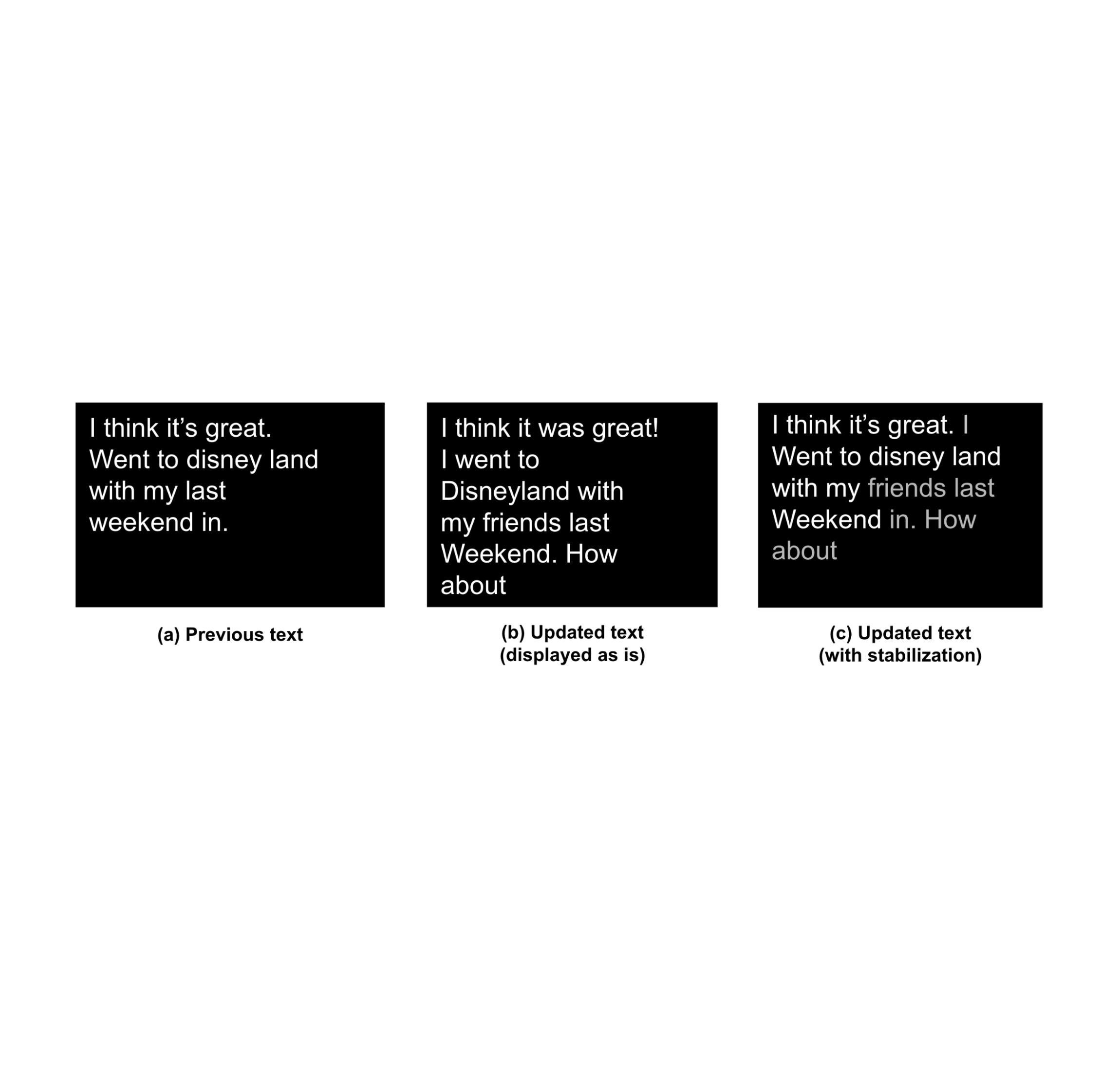
To improve the stability of live captions, we propose an algorithm that takes as input already rendered sequence of tokens (e.g., “Previous” in the figure below) and the new sequence of ASR predictions, and outputs an updated stabilized text (e.g., “Updated text (with stabilization)” below). It considers both the natural language understanding (NLU) aspect as well as the ergonomic aspect (display, layout, etc.) of the user experience in deciding when and how to produce a stable updated text. Specifically, our algorithm performs tokenized alignment, semantic merging, and smooth animation to achieve this goal. In what follows, a token is defined as a word or punctuation produced by ASR.
We show (a) the previously already rendered text, (b) the baseline layout of updated text without our merging algorithm, and (c) the updated text as generated by our stabilization algorithm.
Our algorithm address the challenge of producing stabilized updated text by first identifying three classes of changes (highlighted in red, green, and blue below):
Red: Addition of tokens to the end of previously rendered captions (e.g., "How about'').
Green: Addition / deletion of tokens, in the middle of already rendered captions.
B1: Addition of tokens (e.g., "I'' and "friends''). These may or may not affect the overall comprehension of the captions, but may lead to layout change. Such layout changes are not desired in live captions as they cause significant jitter and poorer user experience. Here “I” does not add to the comprehension but “friends” does. Thus, it is important to balance updates with stability specially for B1 type tokens.
B2: Removal of tokens, e.g., "in'' is removed in the updated sentence.
Blue: Re-captioning of tokens: This includes token edits that may or may not have an impact on the overall comprehension of the captions.
C1: Proper nouns like "disney land'' are updated to "Disneyland''.
C2: Grammatical shorthands like "it's'' are updated to "It was''.
Classes of changes between previously displayed and updated text.
Alignment, merging, and smoothing
To maximize text stability, our goal is to align the old sequence with the new sequence using updates that make minimal changes to the existing layout while ensuring accurate and meaningful captions. To achieve this, we leverage a variant of the Needleman-Wunsch algorithm with dynamic programming to merge the two sequences depending on the class of tokens as defined above:
Case A tokens: We directly add case A tokens, and line breaks as needed to fit the updated captions.
Case B tokens: Our preliminary studies showed that users preferred stability over accuracy for previously displayed captions. Thus, we only update case B tokens if the updates do not break an existing line layout.
Case C tokens: We compare the semantic similarity of case C tokens by transforming original and updated sentences into sentence embeddings, measuring their dot-product, and updating them only if they are semantically different (similarity < 0.85) and the update will not cause new line breaks.
Finally, we leverage animations to reduce visual jitter. We implement smooth scrolling and fading of newly added tokens to further stabilize the overall layout of the live captions.
User evaluation
We conducted a user study with 123 participants to (1) examine the correlation of our proposed flicker metric with viewers’ experience of the live captions, and (2) assess the effectiveness of our stabilization techniques.
We manually selected 20 videos in YouTube to obtain a broad coverage of topics including video conferences, documentaries, academic talks, tutorials, news, comedy, and more. For each video, we selected a 30-second clip with at least 90% speech.
We prepared four types of renderings of live captions to compare:
Raw ASR: raw speech-to-text results from a speech-to-text API.
Raw ASR + thresholding: only display interim speech-to-text result if its confidence score is higher than 0.85.
Stabilized captions: captions using our algorithm described above with alignment and merging.
Stabilized and smooth captions: stabilized captions with smooth animation (scrolling + fading) to assess whether softened display experience helps improve the user experience.
We collected user ratings by asking the participants to watch the recorded live captions and rate their assessments of comfort, distraction, ease of reading, ease of following the video, fatigue, and whether the captions impaired their experience.
Correlation between flicker metric and user experience
We calculated Spearman’s coefficient between the flicker metric and each of the behavioral measurements (values range from -1 to 1, where negative values indicate a negative relationship between the two variables, positive values indicate a positive relationship, and zero indicates no relationship). Shown below, our study demonstrates statistically significant (𝑝 < 0.001) correlations between our flicker metric and users’ ratings. The absolute values of the coefficient are around 0.3, indicating a moderate relationship.
Our proposed technique (stabilized smooth captions) received consistently better ratings, significant as measured by the Mann-Whitney U test (p < 0.01 in the figure below), in five out of six aforementioned survey statements. That is, users considered the stabilized captions with smoothing to be more comfortable and easier to read, while feeling less distraction, fatigue, and impairment to their experience than other types of rendering.
User ratings from 1 (Strongly Disagree) – 7 (Strongly Agree) on survey statements. (**: p<0.01, ***: p<0.001; ****: p<0.0001; ns: non-significant)
Conclusion and future direction
Text instability in live captioning significantly impairs users' reading experience. This work proposes a vision-based metric to model caption stability that statistically significantly correlates with users’ experience, and an algorithm to stabilize the rendering of live captions. Our proposed solution can be potentially integrated into existing ASR systems to enhance the usability of live captions for a variety of users, including those with translation needs or those with hearing accessibility needs.
Our work represents a substantial step towards measuring and improving text stability. This can be evolved to include language-based metrics that focus on the consistency of the words and phrases used in live captions over time. These metrics may provide a reflection of user discomfort as it relates to language comprehension and understanding in real-world scenarios. We are also interested in conducting eye-tracking studies (e.g., videos shown below) to track viewers’ gaze patterns, such as eye fixation and saccades, allowing us to better understand the types of errors that are most distracting and how to improve text stability for those.
Illustration of tracking a viewer’s gaze when reading raw ASR captions.
Illustration of tracking a viewer’s gaze when reading stabilized and smoothed captions.
By improving text stability in live captions, we can create more effective communication tools and improve how people connect in everyday conversations in familiar or, through translation, unfamiliar languages.
Acknowledgements
This work is a collaboration across multiple teams at Google. Key contributors include Xingyu “Bruce” Liu, Jun Zhang, Leonardo Ferrer, Susan Xu, Vikas Bahirwani, Boris Smus, Alex Olwal, and Ruofei Du. We wish to extend our thanks to our colleagues who provided assistance, including Nishtha Bhatia, Max Spear, and Darcy Philippon. We would also like to thank Lin Li, Evan Parker, and CHI 2023 reviewers.
 As a working father with two kids who grew up in the digital era — and as a professional working in online safety outreach and engagement for the last 17 years — I’ve se…


 Chrome is packed with features to help college students stay organized and productive this school year.
 We’re bringing generative AI capabilities in Search (SGE) to more people, making Search Labs available in India and Japan.
 Take a trip to the Forgotten Realms with your Chromebook & NVIDIA’s GeForce NOW cloud gaming service.