Tag Archives: Neural Networks

An NLU-Powered Tool to Explore COVID-19 Scientific Literature


Due to the COVID-19 pandemic, scientists and researchers around the world are publishing an immense amount of new research in order to understand and combat the disease. While the volume of research is very encouraging, it can be difficult for scientists and researchers to keep up with the rapid pace of new publications. Traditional search engines can be excellent resources for finding real-time information on general COVID-19 questions like "How many COVID-19 cases are there in the United States?", but can struggle with understanding the meaning behind research-driven queries. Furthermore, searching through the existing corpus of COVID-19 scientific literature with traditional keyword-based approaches can make it difficult to pinpoint relevant evidence for complex queries.

To help address this problem, we are launching the COVID-19 Research Explorer, a semantic search interface on top of the COVID-19 Open Research Dataset (CORD-19), which includes more than 50,000 journal articles and preprints. We have designed the tool with the goal of helping scientists and researchers efficiently pore through articles for answers or evidence to COVID-19-related questions.

When the user asks an initial question, the tool not only returns a set of papers (like in a traditional search) but also highlights snippets from the paper that are possible answers to the question. The user can review the snippets and quickly make a decision on whether or not that paper is worth further reading. If the user is satisfied with the initial set of papers and snippets, we have added functionality to pose follow-up questions, which act as new queries for the original set of retrieved articles. Take a look at the animation below to see an example of a query and a corresponding follow-up question. We hope these features will foster knowledge exploration and efficient gathering of evidence for scientific hypotheses.

Semantic Search
A key technology powering the tool is semantic search. Semantic search aims to not just capture term overlap between a query and a document, but to really understand whether the meaning of a phrase is relevant to the user’s true intent behind their query.

Consider the query, “What regulates ACE2 expression?” Even though this seems like a simple question, certain phrases can still confuse a search engine that relies solely on text matching. For example, “regulates” can refer to a number of biological processes. While traditional information retrieval (IR) systems use techniques like query expansion to mitigate this confusion, semantic search models aim to learn these relationships implicitly.

Word order also matters. ACE2 (angiotensin converting enzyme-2) itself regulates certain biological processes, but the question is actually asking what regulates ACE2. Matching on terms alone will not distinguish between “what regulates ACE2 ” and “what ACE2 regulates.” Traditional IR systems use tricks like n-gram term matching, but semantic search methods strive to model word order and semantics at their core.

The semantic search technology we use is powered by BERT, which has recently been deployed to improve retrieval quality of Google Search. For the COVID-19 Research Explorer we faced the challenge that biomedical literature uses a language that is very different from the kinds of queries submitted to Google.com. In order to train BERT models, we required supervision — examples of queries and their relevant documents and snippets. While we relied on excellent resources produced by BioASQ for fine-tuning, such human-curated datasets tend to be small. Neural semantic search models require large amounts of training data. To augment small human-constructed datasets, we used advances in query generation to build a large synthetic corpus of questions and relevant documents in the biomedical domain.

Specifically, we used large amounts of general domain question-answer pairs to train an encoder-decoder model (part a in the figure below). This kind of neural architecture is used in tasks like machine translation that encodes one piece of text (e.g., an English sentence) and produces another piece of text (e.g., a French sentence). Here we trained the model to translate from answer passages to questions (or queries) about that passage. Next we took passages from every document in the collection, in this case CORD-19, and generated corresponding queries (part b). We then used these synthetic query-passage pairs as supervision to train our neural retrieval model (part c).
Synthetic query construction.
However, we found that there were examples where the neural model performed worse than a keyword-based model. This is because of the memorization-generalization continuum, which is well known in most fields of artificial intelligence and psycholinguistics. Keyword-based models, like tf-idf, are essentially memorizers. They memorize terms from the query and look for documents that have them. Neural retrieval models, on the other hand, learn generalizations about concepts and meaning and try to match based on those. Sometimes they can over-generalize when precision is important. For example, if I query, “What regulates ACE2 expression?”, one may want the model to generalize the concept of “regulation,” but not ACE2 beyond acronym expansion.

Hybrid Term-Neural Retrieval Model
To improve our system we built a hybrid term-neural retrieval model. A crucial observation is that both term-based and neural models can be cast as a vector space model. In other words, we can encode both the query and documents and then treat retrieval as looking for the document vectors that are most similar to the query vector, also known as k-nearest neighbor retrieval. There is a lot of research and engineering that is needed to make this work at scale, but it allows us a simple mechanism to combine methods. The simplest approach is to combine the vectors with a trade-off parameter.
Hybrid Term and Neural Retrieval.
In the figure above, the blue boxes are the term-based vectors, and the red, the neural vectors. We represent documents by concatenating these vectors. We concatenate the two vectors for queries as well, but we control the relative importance of exact term matches versus neural semantic matching. This is done via a weight parameter k. While more complex hybrid schemes are possible, we found that this simple hybrid model significantly increased quality on our biomedical literature retrieval benchmarks.

Availability and Community Feedback
The COVID-19 Research Explorer is freely available to the research community as an open alpha. Over the coming months we will be making a number of usability enhancements, so please check back often. Try out the COVID-19 Research Explorer, and please share any comments you have with us via the feedback channels on the site.

Acknowledgements
This effort has been successful thanks to the hard work of many people, including, but not limited to the following (in alphabetical order of last name): John Alex, Waleed Ammar, Greg Billock, Yale Cong, Ali Elkahky, Daniel Francisco, Stephen Greco, Stefan Hosein, Johanna Katz, Gyorgy Kiss, Margarita Kopniczky, Ivan Korotkov, Dominic Leung, Daphne Luong, Ji Ma, Ryan Mcdonald, Matt Pearson-Beck, Biao She, Jonathan Sheffi, Kester Tong, Ben Wedin

Source: Google AI Blog


Fast and Easy Infinitely Wide Networks with Neural Tangents


The widespread success of deep learning across a range of domains such as natural language processing, conversational agents, and connectomics, has transformed the landscape of research in machine learning and left researchers with a number of interesting and important open questions such as: Why do deep neural networks (DNNs) generalize so well despite being overparameterized? What is the relationship between architecture, training, and performance for deep networks? How can one extract salient features from deep learning models?

One of the key theoretical insights that has allowed us to make progress in recent years has been that increasing the width of DNNs results in more regular behavior, and makes them easier to understand. A number of recent results have shown that DNNs that are allowed to become infinitely wide converge to another, simpler, class of models called Gaussian processes. In this limit, complicated phenomena (like Bayesian inference or gradient descent dynamics of a convolutional neural network) boil down to simple linear algebra equations. Insights from these infinitely wide networks frequently carry over to their finite counterparts. As such, infinite-width networks can be used as a lens to study deep learning, but also as useful models in their own right.
Left: A schematic showing how deep neural networks induce simple input / output maps as they become infinitely wide. Right: As the width of a neural network increases , we see that the distribution of outputs over different random instantiations of the network becomes Gaussian.
Unfortunately, deriving the infinite-width limit of a finite network requires significant mathematical expertise and has to be worked out separately for each architecture studied. Once the infinite-width model is derived, coming up with an efficient and scalable implementation further requires significant engineering proficiency. Together, the process of taking a finite-width model to its corresponding infinite-width network could take months and might be the topic of a research paper in its own right.

To address this issue and to accelerate theoretical progress in deep learning, we present Neural Tangents, a new open-source software library written in JAX that allows researchers to build and train infinitely wide neural networks as easily as finite neural networks. At its core, Neural Tangents provides an easy-to-use neural network library that builds finite- and infinite-width versions of neural networks simultaneously.

As an example of the utility of Neural Tangents, imagine training a fully-connected neural network on some data. Normally, a neural network is randomly initialized and then trained using gradient descent. Initializing and training many of these neural networks results in an ensemble. Often researchers and practitioners average the predictions from different members of the ensemble together for better performance. Additionally, the variance in the predictions of members of the ensemble can be used to estimate uncertainty. The downside is that training an ensemble of networks requires a significant computational budget, so it is often avoided. However, when the neural networks become infinitely wide, the ensemble is described by a Gaussian process with a mean and variance that can be computed throughout training.

With Neural Tangents, one can construct and train ensembles of these infinite-width networks at once using only five lines of code! The resulting training process is displayed below, and an interactive colaboratory notebook going through this experiment can be found here.
In both plots we compare training of an ensemble of finite neural networks with the infinite-width ensemble of the same architecture. The empirical mean and variance of the finite ensemble is displayed as a dashed black line between two dotted black lines. The closed-form mean and variance of the infinite-width ensemble is displayed as a solid colored line inside a filled color region. In both plots finite- and infinite-width ensembles match very closely and can be hard to distinguish. Left: Outputs (vertical f-axis) on the input data (horizontal x-axis) as the training progresses. Right: Train and test loss with uncertainty over the course of training.
Despite the fact that the infinite-width ensemble is governed by a simple closed-form expression, it exhibits remarkable agreement with the finite-width ensemble. And since the infinite-width ensemble is a Gaussian process, it naturally provides closed-form uncertainty estimates (filled colored regions in the figure above). These uncertainty estimates closely match the variation of predictions that are observed when training many different copies of the finite network (dashed lines).

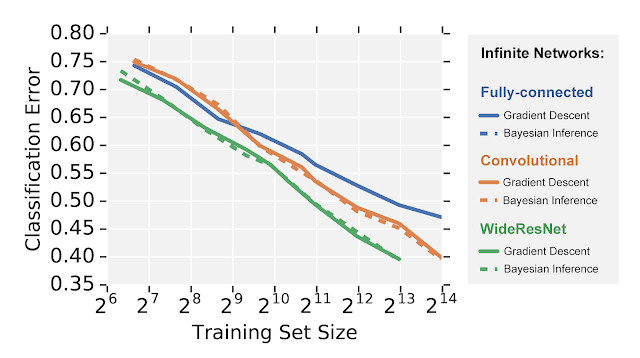
The above example shows the power of infinite-width neural networks to capture training dynamics. However, networks built using Neural Tangents can be applied to any problem on which you could apply a regular neural network. For example, below we compare three different infinite-width neural network architectures on image recognition using the CIFAR-10 dataset. Remarkably, we can evaluate ensembles of highly-elaborate models like infinitely wide residual networks in closed-form under both gradient descent and fully-Bayesian inference (an intractable task in the finite-width regime).
We see that, mimicking finite neural networks, infinite-width networks follow a similar hierarchy of performance with fully-connected networks performing worse than convolutional networks, which in turn perform worse than wide residual networks. However, unlike regular training, the learning dynamics of these models is completely tractable in closed-form, which allows unprecedented insight into their behavior.

We invite everyone to explore the infinite-width versions of their models with Neural Tangents, and help us open the black box of deep learning. To get started, please check out the paper, the tutorial Colab notebook, and the Github repo — contributions, feature requests, and bug reports are very welcome. This work has been accepted as a spotlight at ICLR 2020.

Acknowledgements
Neural Tangents is being actively developed by Lechao Xiao, Roman Novak, Jiri Hron, Jaehoon Lee, Alex Alemi, Jascha Sohl-Dickstein, and Samuel S. Schoenholz. We also thank Yasaman Bahri and Greg Yang for the ongoing contributions to improve the library, as well as Sergey Ioffe, Ben Adlam, Ravid Ziv, and Jeffrey Pennington for frequent discussion and useful feedback. Finally, we thank Tom Small for creating the animation in the first figure.

Source: Google AI Blog


Understanding Transfer Learning for Medical Imaging


As deep neural networks are applied to an increasingly diverse set of domains, transfer learning has emerged as a highly popular technique in developing deep learning models. In transfer learning, the neural network is trained in two stages: 1) pretraining, where the network is generally trained on a large-scale benchmark dataset representing a wide diversity of labels/categories (e.g., ImageNet); and 2) fine-tuning, where the pretrained network is further trained on the specific target task of interest, which may have fewer labeled examples than the pretraining dataset. The pretraining step helps the network learn general features that can be reused on the target task.

This kind of two-stage paradigm has become extremely popular in many settings, and particularly so in medical imaging. In the context of transfer learning, standard architectures designed for ImageNet with corresponding pretrained weights are fine-tuned on medical tasks ranging from interpreting chest x-rays and identifying eye diseases, to early detection of Alzheimer’s disease. Despite its widespread use, however, the precise effects of transfer learning are not yet well understood. While recent work challenges many common assumptions, including the effects on performance improvement, contribution of the underlying architecture and impact of pretraining dataset type and size, these results are all in the natural image setting, and leave many questions open for specialized domains, such as medical images.

In our NeurIPS 2019 paper, “Transfusion: Understanding Transfer Learning for Medical Imaging,” we investigate these central questions for transfer learning in medical imaging tasks. Through both a detailed performance evaluation and analysis of neural network hidden representations, we uncover many surprising conclusions, such as the limited benefits of transfer learning for performance on the tested medical imaging tasks, a detailed characterization of how representations evolve through the training process across different models and hidden layers, and feature independent benefits of transfer learning for convergence speed.

Performance Evaluation
We first performed a thorough study on the effect of transfer learning on model performance. We compared models trained from random initialization and applied directly on tasks to those pretrained on ImageNet that leverage transfer learning for the same tasks. We looked at two large scale medical imaging tasks — diagnosing diabetic retinopathy from fundus photographs and identifying five different diseases from chest x-rays. We evaluated various neural network architectures including both standard architectures popularly used for medical imaging (ResNet50, Inception-v3) as well as a family of simple, lightweight convolutional neural networks that consist of four or five layers of the standard convolution-batchnorm-ReLU progression, or CBRs.

The results from evaluating all of these models on the different tasks with and without transfer learning give us four main takeaways:
  • Surprisingly, transfer learning does not significantly affect performance on medical imaging tasks, with models trained from scratch performing nearly as well as standard ImageNet transferred models.
  • On the medical imaging tasks, the much smaller CBR models perform at a level comparable to the standard ImageNet architectures.
  • As the CBR models are much smaller and shallower than the standard ImageNet models, they perform much worse on ImageNet classification, highlighting that ImageNet performance is not indicative of performance on medical tasks.
  • The two medical tasks are much smaller in size than ImageNet (~200k vs ~1.2m training images), but in the very small data regime, there may only be a few thousand training examples. We evaluated transfer learning in this very small data regime, finding that while there was a larger gap in performance between transfer and training from scratch for large models (ResNet) this was not true for smaller models (CBRs), suggesting that the large models designed for ImageNet might be too overparameterized for the very small data regime.
Representation Analysis
We next study the degree to which transfer learning affects the kinds of features and representations learned by the neural networks. Given the similar performance, does transfer learning result in different representations from random initialization? Is knowledge from the pretraining step reused, and if so, where? To find answers to these questions, this study analyzes and compares the hidden representations (i.e., representations learned in the latent layers of the network) in the different neural networks trained to solve these tasks. This quantitative analysis can be challenging, due to the complexity and lack of alignment in different hidden layers. But a recent method, singular vector canonical correlation analysis (SVCCA; code and tutorials), based on canonical correlation analysis (CCA), helps overcome these challenges, and can be used to calculate a similarity score between a pair of hidden representations.

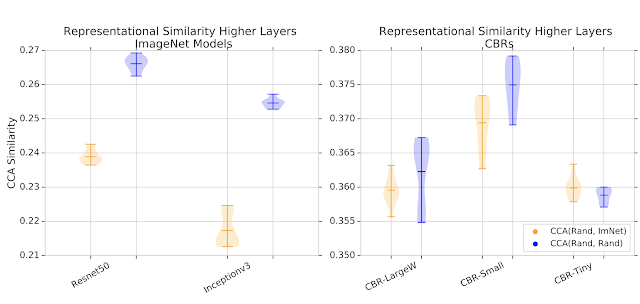
Similarity scores are computed for some of the hidden representations from the top latent layers of the networks (closer to the output) between networks trained from random initialization and networks trained from pretrained ImageNet weights. As a baseline, we also compute similarity scores of representations learned from different random initializations. For large models, representations learned from random initialization are much more similar to each other than those learned from transfer learning. For smaller models, there is greater overlap between representation similarity scores.
Representation similarity scores between networks trained from random initialization and networks trained from pretrained ImageNet weights (orange), and baseline similarity scores of representations trained from two different random initializations (blue). Higher values indicate greater similarity. For larger models, representations learned from random initialization are much more similar to each other than those learned through transfer. This is not the case for smaller models.
The reason for this difference between large and small models becomes clear with further investigation into the hidden representations. Large models change less through training, even from random initialization. We perform multiple experiments that illustrate this, from simple filter visualizations to tracking changes between different layers through fine-tuning.

When we combine the results of all the experiments from the paper, we can assemble a table summarizing how much representations change through training on the medical task across (i) transfer learning, (ii) model size and (iii) lower/higher layers.
Effects on Convergence: Feature Independent Benefits and Hybrid Approaches
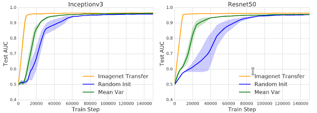
One consistent effect of transfer learning was a significant speedup in the time taken for the model to converge. But having seen the mixed results for feature reuse from our representational study, we looked into whether there were other properties of the pretrained weights that might contribute to this speedup. Surprisingly, we found a feature independent benefit of pretraining — the weight scaling.

We initialized the weights of the neural network as independent and identically distributed (iid), just like random initialization, but using the mean and variance of the pretrained weights. We called this initialization the Mean Var Init, which keeps the pretrained weight scaling but destroys all the features. This Mean Var Init offered significant speedups over random initialization across model architectures and tasks, suggesting that the pretraining process of transfer learning also helps with good weight conditioning.
Filter visualization of weights initialized according to pretrained ImageNet weights, Random Init, and Mean Var Init. Only the ImageNet Init filters have pretrained (Gabor-like) structure, as Rand Init and Mean Var weights are iid.
Recall that our earlier experiments suggested that feature reuse primarily occurs in the lowest layers. To understand this, we performed weight transfusion experiments, where only a subset of the pretrained weights (corresponding to a contiguous set of layers) are transferred, with the remainder of weights being randomly initialized. Comparing convergence speeds of these transfused networks with full transfer learning further supports the conclusion that feature reuse is primarily happening in the lowest layers.
Learning curves comparing the convergence speed with AUC on the test set. Using only the scaling of the pretrained weights (Mean Var Init) helps with convergence speed. The figures compare the standard transfer learning and the Mean Var initialization scheme to training from random initialization.
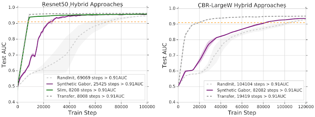
This suggests hybrid approaches to transfer learning, where instead of reusing the full neural network architecture, we can recycle its lowest layers and redesign the upper layers to better suit the target task. This gives us most of the benefits of transfer learning while further enabling flexible model design. In the Figure below, we show the effect of reusing pretrained weights up to Block2 in Resnet50, halving the remainder of the channels, initializing those layers randomly, and then training end-to-end. This matches the performance and convergence of full transfer learning.
Hybrid approaches to transfer learning on Resnet50 (left) and CBR models (right) — reusing a subset of the weights and slimming the remainder of the network (Slim), and using mathematically synthesized Gabors for conv1 (Synthetic Gabor).
The figure above also shows the results of an extreme version of this partial reuse, transferring only the very first convolutional layer with mathematically synthesized Gabor filters (pictured below). Using just these (synthetic) weights offers significant speedups, and hints at many other creative hybrid approaches.
Synthetic Gabor filters used to initialize the first layer if neural networks in some of the experiments in this paper. The Gabor filters are generated as grayscale images and repeated across the RGB channels. Left: Low frequencies. Right: High frequencies.
Conclusion and Open Questions
Transfer learning is a central technique for many domains. In this paper we provide insights on some of its fundamental properties in the medical imaging context, studying performance, feature reuse, the effect of different architectures, convergence and hybrid approaches. Many interesting open questions remain: How much of the original task has the model forgotten? Why do large models change less? Can we get further gains matching higher order moments of pretrained weight statistics? Are the results similar for other tasks, such as segmentation? We look forward to tackling these questions in future work!

Acknowledgements
Special thanks to Samy Bengio and Jon Kleinberg, who are co-authors on this work. Thanks also to Geoffrey Hinton for helpful feedback.

Source: Google AI Blog


Exploring Weight Agnostic Neural Networks


When training a neural network to accomplish a given task, be it image classification or reinforcement learning, one typically refines a set of weights associated with each connection within the network. Another approach to creating successful neural networks that has shown substantial progress is neural architecture search, which constructs neural network architectures out of hand-engineered components such as convolutional network components or transformer blocks. It has been shown that neural network architectures built with these components, such as deep convolutional networks, have strong inductive biases for image processing tasks, and can even perform them when their weights are randomly initialized. While neural architecture search produces new ways of arranging hand-engineered components with known inductive biases for the task domain at hand, there has been little progress in the automated discovery of new neural network architectures with such inductive biases, for various task domains.

We can look at analogies to these useful components in examples of nature vs. nurture. Just as certain precocial species in biology—who possess anti-predator behaviors from the moment of birth—can perform complex motor and sensory tasks without learning, perhaps we can construct network architectures that can perform well without training. Of course, these natural (and by analogy, artificial) neural networks are further improved through training, but their ability to perform even without learning shows that they contain biases that make them well-suited to their task.

In “Weight Agnostic Neural Networks” (WANN), we present a first step toward searching specifically for networks with these biases: neural net architectures that can already perform various tasks, even when they use a random shared weight. Our motivation in this work is to question to what extent neural network architectures alone, without learning any weight parameters, can encode solutions for a given task. By exploring such neural network architectures, we present agents that can already perform well in their environment without the need to learn weight parameters. Furthermore, in order to spur progress in this field community, we have also open-sourced the code to reproduce our WANN experiments for the broader research community.
Left: A hand-engineered, fully-connected deep neural network with 2760 weight connections. Using a learning algorithm, we can solve for the set of 2760 weight parameters so that this network can perform the BipedalWalker-v2 task. Right: A weight agnostic neural network architecture with 44 connections that can perform the same Bipedal Walker task. Unlike the fully-connected network, this WANN can still perform the task without the need to train the weight parameters of each connection. In fact, to simplify the training, the WANN is designed to perform when the values of each weight connection are identical, or shared, and it will even function if this shared weight parameter is randomly sampled.
Finding WANNs
We start with a population of minimal neural network architecture candidates, each with very few connections only, and use a well-established topology search algorithm (NEAT), to evolve the architectures by adding single connections and single nodes one by one. The key idea behind WANNs is to search for architectures by de-emphasizing weights. Unlike traditional neural architecture search methods, where all of the weight parameters of new architectures need to be trained using a learning algorithm, we take a simpler and more efficient approach. Here, during the search, all candidate architectures are first assigned a single shared weight value at each iteration, and then optimized to perform well over a wide range of shared weight values.
Operators for searching the space of network topologies
Left: A minimal network topology, with input and outputs only partially connected.
Middle: Networks are altered in one of three ways:
(1) Insert Node: a new node is inserted by splitting an existing connection.
(2) Add Connection: a new connection is added by connecting two previously unconnected nodes.
(3) Change Activation: the activation function of a hidden node is reassigned.
Right: Possible activation functions (linear, step, sin, cosine, Gaussian, tanh, sigmoid, inverse, absolute value, ReLU)
In addition to exploring a range of weight agnostic neural networks, it is important to also look for network architectures that are only as complex as they need to be. We accomplish this by optimizing for both the performance of the networks and their complexity simultaneously, using techniques drawn from multi-objective optimization.
Overview of Weight Agnostic Neural Network Search and corresponding operators for searching the space of network topologies.
Training WANN Architectures
Unlike traditional networks, we can easily train the WANN by simply finding the best single shared weight parameter that maximizes its performance. In the example below, we see that our architecture works (to some extent) for a swing-up cartpole task using constant weights:
A WANN performing a Cartpole Swing-up task at various different weight parameters, and also using fine-tuned weight parameters.
As we see in the above figure, while WANNs can perform its task using range of shared weight parameters, the performance is still not comparable to a network that learns weights for each individual connection, as normally done in network training. If we want to further improve its performance, we can use the WANN architecture, and the best shared weight as a starting point to fine-tune the weights of each individual connection using a learning algorithm, like how we would normally train any neural network. Using the weight agnostic property of the network architecture as a starting point, and fine-tuning its performance via learning, may help provide insightful analogies to how animals learn.
Through the use of multi-objective optimization for both performance and network simplicity, our method found a simple WANN for a Car Racing from pixels task that works well without explicitly training for the weights of the network.
The ability for a network architecture to function using only random weights offers other advantages too. For instance, by using copies of the same WANN architecture, but where each copy of the WANN is assigned a different distinct weight value, we can create an ensemble of multiple distinct models for the same task. This ensemble generally achieves better performance than a single model. We illustrate this with an example of an MNIST classifier evolved to work with random weights:
An MNIST classifier evolved to work with random weights.
While a conventional network with random initialization will achieve ~10% accuracy on MNIST, this particular network architecture uses random weights and when applied to MNIST achieves an accuracy much better than chance (> 80%). When an ensemble of WANNs is used, each of which assigned with a different shared weight, the accuracy increases to > 90%.

Even without ensemble methods, collapsing the number of weight values in a network to one allows the network to be rapidly tuned. The ability to quickly fine-tune weights might be useful in continual lifelong learning, where agents acquire, adapt, and transfer skills throughout their lifespan. This makes WANNs particularly well positioned to exploit the Baldwin effect, the evolutionary pressure that rewards individuals predisposed to learn useful behaviors, without being trapped in the computationally expensive trap of ‘learning to learn’.

Conclusion
We hope that this work can serve as a stepping stone to help discover novel fundamental neural network components such as the convolutional network, whose discovery and application have been instrumental to the incredible progress made in deep learning. The computational resources available to the research community have grown significantly since the time convolutional neural networks were discovered. If we are devoting such resources to automated discovery and hope to achieve more than incremental improvements in network architectures, we believe it is also worth searching for with new building blocks, not just their arrangements.

If you are interested to learn more about this work, we invite readers to read our interactive article (or pdf version of the paper for offline reading). In addition to open sourcing these experiments to the research community, we have also released a general Python implementation of NEAT called PrettyNEAT to help interested readers to explore the exciting area of neural network evolution from first principles.

Source: Google AI Blog


Parrotron: New Research into Improving Verbal Communication for People with Speech Impairments


Most people take for granted that when they speak, they will be heard and understood. But for the millions who live with speech impairments caused by physical or neurological conditions, trying to communicate with others can be difficult and lead to frustration. While there have been a great number of recent advances in automatic speech recognition (ASR; a.k.a. speech-to-text) technologies, these interfaces can be inaccessible for those with speech impairments. Further, applications that rely on speech recognition as input for text-to-speech synthesis (TTS) can exhibit word substitution, deletion, and insertion errors. Critically, in today’s technological environment, limited access to speech interfaces, such as digital assistants that depend on directly understanding one's speech, means being excluded from state-of-the-art tools and experiences, widening the gap between what those with and without speech impairments can access.

Project Euphonia has demonstrated that speech recognition models can be significantly improved to better transcribe a variety of atypical and dysarthric speech. Today, we are presenting Parrotron, an ongoing research project that continues and extends our effort to build speech technologies to help those with impaired or atypical speech to be understood by both people and devices. Parrotron consists of a single end-to-end deep neural network trained to convert speech from a speaker with atypical speech patterns directly into fluent synthesized speech, without an intermediate step of generating text—skipping speech recognition altogether. Parrotron’s approach is speech-centric, looking at the problem only from the point of view of speech signals—e.g., without visual cues such as lip movements. Through this work, we show that Parrotron can help people with a variety of atypical speech patterns—including those with ALS, deafness, and muscular dystrophy—to be better understood in both human-to-human interactions and by ASR engines.
The Parrotron Speech Conversion Model
Parrotron is an attention-based sequence-to-sequence model trained in two phases using parallel corpora of input/output speech pairs. First, we build a general speech-to-speech conversion model for standard fluent speech, followed by a personalization phase that adjusts the model parameters to the atypical speech patterns from the target speaker. The primary challenge in such a configuration lies in the collection of the parallel training data needed for supervised training, which consists of utterances spoken by many speakers and mapped to the same output speech content spoken by a single speaker. Since it is impractical to have a single speaker record the many hours of training data needed to build a high quality model, Parrotron uses parallel data automatically derived with a TTS system. This allows us to make use of a pre-existing anonymized, transcribed speech recognition corpus to obtain training targets.

The first training phase uses a corpus of ~30,000 hours that consists of millions of anonymized utterance pairs. Each pair includes a natural utterance paired with an automatically synthesized speech utterance that results from running our state-of-the-art Parallel WaveNet TTS system on the transcript of the first. This dataset includes utterances from thousands of speakers spanning hundreds of dialects/accents and acoustic conditions, allowing us to model a large variety of voices, linguistic and non-linguistic contents, accents, and noise conditions with “typical” speech all in the same language. The resulting conversion model projects away all non-linguistic information, including speaker characteristics, and retains only what is being said, not who, where, or how it is said. This base model is used to seed the second personalization phase of training.

The second training phase utilizes a corpus of utterance pairs generated in the same manner as the first dataset. In this case, however, the corpus is used to adapt the network to the acoustic/phonetic, phonotactic and language patterns specific to the input speaker, which might include, for example, learning how the target speaker alters, substitutes, and reduces or removes certain vowels or consonants. To model ALS speech characteristics in general, we use utterances taken from an ALS speech corpus derived from Project Euphonia. If instead we want to personalize the model for a particular speaker, then the utterances are contributed by that person. The larger this corpus is, the better the model is likely to be at correctly converting to fluent speech. Using this second smaller and personalized parallel corpus, we run the neural-training algorithm, updating the parameters of the pre-trained base model to generate the final personalized model.

We found that training the model with a multitask objective to predict the target phonemes while simultaneously generating spectrograms of the target speech led to significant quality improvements. Such a multitask trained encoder can be thought of as learning a latent representation of the input that maintains information about the underlying linguistic content.
Overview of the Parrotron model architecture. An input speech spectrogram is passed through encoder and decoder neural networks to generate an output spectrogram in a new voice.
Case Studies
To demonstrate a proof of concept, we worked with our fellow Google research scientist and mathematician Dimitri Kanevsky, who was born in Russia to Russian speaking, normal-hearing parents but has been profoundly deaf from a very young age. He learned to speak English as a teenager, by using Russian phonetic representations of English words, learning to pronounce English using transliteration into Russian (e.g., The quick brown fox jumps over the lazy dog => ЗИ КВИК БРАУН ДОГ ЖАМПС ОУВЕР ЛАЙЗИ ДОГ). As a result, Dimitri’s speech is substantially distinct from native English speakers, and can be challenging to comprehend for systems or listeners who are not accustomed to it.

Dimitri recorded a corpus of 15 hours of speech, which was used to adapt the base model to the nuances specific to his speech. The resulting Parrotron system helped him be better understood by both people and Google’s ASR system alike. Running Google’s ASR engine on the output of Parrotron significantly reduced the word error rate from 89% to 32%, on a held out test set from Dimitri. Below is an example of Parrotron’s successful conversion of input speech from Dimitri:

Input from Dimitri Audio
Output from Parrotron Audio

We also worked with Aubrie Lee, a Googler and advocate for disability inclusion, who has muscular dystrophy, a condition that causes progressive muscle weakness, and sometimes impacts speech production. Aubrie contributed 1.5 hours of speech, which has been instrumental in showing promising outcomes of the applicability of this speech-to-speech technology. Below is an example of Parrotron’s successful conversion of input speech from Aubrie:

Input from Aubrie Audio
Output from Parrotron Audio
Input from Aubrie Audio
Output from Parrotron Audio

We also tested Parrotron’s performance on speech from speakers with ALS by adapting the pretrained model on multiple speakers who share similar speech characteristics grouped together, rather than on a single speaker. We conducted a preliminary listening study and observed an increase in intelligibility when comparing natural ALS speech to the corresponding speech obtained from running the Parroton model, for the majority of our test speakers.

Cascaded Approach
Project Euphonia has built a personalized speech-to-text model that has reduced the word error rate for a deaf speaker from 89% to 25%, and ongoing research is also likely to improve upon these results. One could use such a speech-to-text model to achieve a similar goal as Parrotron by simply passing its output into a TTS system to synthesize speech from the result. In such a cascaded approach, however, the recognizer may choose an incorrect word (roughly 1 out 4 times, in this case)—i.e., it may yield words/sentences with unintended meaning and, as a result, the synthesized audio of these words would be far from the speaker’s intention. Given the end-to-end speech-to-speech training objective function of Parrotron, even when errors are made, the generated output speech is likely to sound acoustically similar to the input speech, and thus the speaker’s original intention is less likely to be significantly altered and it is often still possible to understand what is intended:

Input from Dimitri Audio
Output from Parrotron Audio
Input from Dimitri Audio
Output from Parrotron/Input to Assistant Audio
Output from Assistant Audio
Input from Aubrie Audio
Output from Parrotron Audio

Furthermore, since Parrotron is not strongly biased to producing words from a predefined vocabulary set, input to the model may contain completely new invented words, foreign words/names, and even nonsense words. We observe that feeding Arabic and Spanish utterances into the US-English Parrotron model often results in output which echoes the original speech content with an American accent, in the target voice. Such behavior is qualitatively different from what one would obtain by simply running an ASR followed by a TTS. Finally, by going from a combination of independently tuned neural networks to a single one, we also believe there are improvements and simplifications that could be substantial.

Conclusion
Parrotron makes it easier for users with atypical speech to talk to and be understood by other people and by speech interfaces, with its end-to-end speech conversion approach more likely to reproduce the user’s intended speech. More exciting applications of Parrotron are discussed in our paper and additional audio samples can be found on our github repository. If you would like to participate in this ongoing research, please fill out this short form and volunteer to record a set of phrases. We look forward to working with you!
Acknowledgements
This project was joint work between the Speech and Google Brain teams. Contributors include Fadi Biadsy, Ron Weiss, Pedro Moreno, Dimitri Kanevsky, Ye Jia, Suzan Schwartz, Landis Baker, Zelin Wu, Johan Schalkwyk, Yonghui Wu, Zhifeng Chen, Patrick Nguyen, Aubrie Lee, Andrew Rosenberg, Bhuvana Ramabhadran, Jason Pelecanos, Julie Cattiau, Michael Brenner, Dotan Emanuel and Joel Shor. Our data collection efforts have been vastly accelerated by our collaborations with ALS-TDI.

Source: Google AI Blog


SpecAugment: A New Data Augmentation Method for Automatic Speech Recognition


Automatic Speech Recognition (ASR), the process of taking an audio input and transcribing it to text, has benefited greatly from the ongoing development of deep neural networks. As a result, ASR has become ubiquitous in many modern devices and products, such as Google Assistant, Google Home and YouTube. Nevertheless, there remain many important challenges in developing deep learning-based ASR systems. One such challenge is that ASR models, which have many parameters, tend to overfit the training data and have a hard time generalizing to unseen data when the training set is not extensive enough.

In the absence of an adequate volume of training data, it is possible to increase the effective size of existing data through the process of data augmentation, which has contributed to significantly improving the performance of deep networks in the domain of image classification. In the case of speech recognition, augmentation traditionally involves deforming the audio waveform used for training in some fashion (e.g., by speeding it up or slowing it down), or adding background noise. This has the effect of making the dataset effectively larger, as multiple augmented versions of a single input is fed into the network over the course of training, and also helps the network become robust by forcing it to learn relevant features. However, existing conventional methods of augmenting audio input introduces additional computational cost and sometimes requires additional data.

In our recent paper, “SpecAugment: A Simple Data Augmentation Method for Automatic Speech Recognition”, we take a new approach to augmenting audio data, treating it as a visual problem rather than an audio one. Instead of augmenting the input audio waveform as is traditionally done, SpecAugment applies an augmentation policy directly to the audio spectrogram (i.e., an image representation of the waveform). This method is simple, computationally cheap to apply, and does not require additional data. It is also surprisingly effective in improving the performance of ASR networks, demonstrating state-of-the-art performance on the ASR tasks LibriSpeech 960h and Switchboard 300h.

SpecAugment
In traditional ASR, the audio waveform is typically encoded as a visual representation, such as a spectrogram, before being input as training data for the network. Augmentation of training data is normally applied to the waveform audio before it is converted into the spectrogram, such that after every iteration, new spectrograms must be generated. In our approach, we investigate the approach of augmenting the spectrogram itself, rather than the waveform data. Since the augmentation is applied directly to the input features of the network, it can be run online during training without significantly impacting training speed.
A waveform is typically converted into a visual representation (in our case, a log mel spectrogram; steps 1 through 3 of this article) before being fed into a network.
SpecAugment modifies the spectrogram by warping it in the time direction, masking blocks of consecutive frequency channels, and masking blocks of utterances in time. These augmentations have been chosen to help the network to be robust against deformations in the time direction, partial loss of frequency information and partial loss of small segments of speech of the input. An example of such an augmentation policy is displayed below.
The log mel spectrogram is augmented by warping in the time direction, and masking (multiple) blocks of consecutive time steps (vertical masks) and mel frequency channels (horizontal masks). The masked portion of the spectrogram is displayed in purple for emphasis.
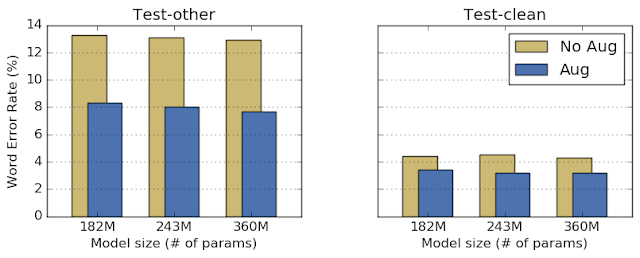
To test SpecAugment, we performed some experiments with the LibriSpeech dataset, where we took three Listen Attend and Spell (LAS) networks, end-to-end networks commonly used for speech recognition, and compared the test performance between networks trained with and without augmentation. The performance of an ASR network is measured by the Word Error Rate (WER) of the transcript produced by the network against the target transcript. Here, all hyperparameters were kept the same, and only the data fed into the network was altered. We found that SpecAugment improves network performance without any additional adjustments to the network or training parameters.
Performance of networks on the test sets of LibriSpeech with and without augmentation. The LibriSpeech test set is divided into two portions, test-clean and test-other, the latter of which contains noisier audio data.
More importantly, SpecAugment prevents the network from over-fitting by giving it deliberately corrupted data. As an example of this, below we show how the WER for the training set and the development (or dev) set evolves through training with and without augmentation. We see that without augmentation, the network achieves near-perfect performance on the training set, while grossly under-performing on both the clean and noisy dev set. On the other hand, with augmentation, the network struggles to perform as well on the training set, but actually shows better performance on the clean dev set, and shows comparable performance on the noisy dev set. This suggests that the network is no longer over-fitting the training data, and that improving training performance would lead to better test performance.
Training, clean (dev-clean) and noisy (dev-other) development set performance with and without augmentation.
State-of-the-Art Results
We can now focus on improving training performance, which can be done by adding more capacity to the networks by making them larger. By doing this in conjunction with increasing training time, we were able to get state-of-the-art (SOTA) results on the tasks LibriSpeech 960h and Switchboard 300h.
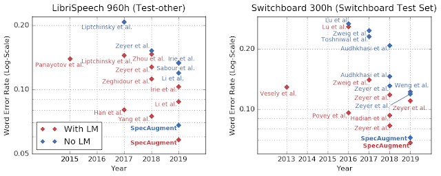
Word error rates (%) for state-of-the-art results for the tasks LibriSpeech 960h and Switchboard 300h. The test set for both tasks have a clean (clean/Switchboard) and a noisy (other/CallHome) subset. Previous SOTA results taken from Li et. al (2019), Yang et. al (2018) and Zeyer et. al (2018).
The simple augmentation scheme we have used is surprisingly powerful—we are able to improve the performance of the end-to-end LAS networks so much that it surpasses those of classical ASR models, which traditionally did much better on smaller academic datasets such as LibriSpeech or Switchboard.
Performance of various classes of networks on LibriSpeech and Switchboard tasks. The performance of LAS models is compared to classical (e.g., HMM) and other end-to-end models (e.g., CTC/ASG) over time.
Language Models
Language models (LMs), which are trained on a bigger corpus of text-only data, have played a significant role in improving the performance of an ASR network by leveraging information learned from text. However, LMs typically need to be trained separately from the ASR network, and can be very large in memory, making it hard to fit on a small device, such as a phone. An unexpected outcome of our research was that models trained with SpecAugment out-performed all prior methods even without the aid of a language model. While our networks still benefit from adding an LM, our results are encouraging in that it suggests the possibility of training networks that can be used for practical purposes without the aid of an LM.
Word error rates for LibriSpeech and Switchboard tasks with and without LMs. SpecAugment outperforms previous state-of-the-art even before the inclusion of a language model.
Most of the work on ASR in the past has been focused on looking for better networks to train. Our work demonstrates that looking for better ways to train networks is a promising alternative direction of research.

Acknowledgements
We would like to thank the co-authors of our paper Chung-Cheng Chiu, Ekin Dogus Cubuk, Quoc Le, Yu Zhang and Barret Zoph. We also thank Yuan Cao, Ciprian Chelba, Kazuki Irie, Ye Jia, Anjuli Kannan, Patrick Nguyen, Vijay Peddinti, Rohit Prabhavalkar, Yonghui Wu and Shuyuan Zhang for useful discussions.

Source: Google AI Blog


MorphNet: Towards Faster and Smaller Neural Networks


Deep neural networks (DNNs) have demonstrated remarkable effectiveness in solving hard problems of practical relevance such as image classification, text recognition and speech transcription. However, designing a suitable DNN architecture for a given problem continues to be a challenging task. Given the large search space of possible architectures, designing a network from scratch for your specific application can be prohibitively expensive in terms of computational resources and time. Approaches such as Neural Architecture Search and AdaNet use machine learning to search the design space in order to find improved architectures. An alternative is to take an existing architecture for a similar problem and, in one shot, optimize it for the task at hand.

Here we describe MorphNet, a sophisticated technique for neural network model refinement, which takes the latter approach. Originally presented in our paper, “MorphNet: Fast & Simple Resource-Constrained Structure Learning of Deep Networks”, MorphNet takes an existing neural network as input and produces a new neural network that is smaller, faster, and yields better performance tailored to a new problem. We've applied the technique to Google-scale problems to design production-serving networks that are both smaller and more accurate, and now we have open sourced the TensorFlow implementation of MorphNet to the community so that you can use it to make your models more efficient.

How it Works
MorphNet optimizes a neural network through a cycle of shrinking and expanding phases. In the shrinking phase, MorphNet identifies inefficient neurons and prunes them from the network by applying a sparsifying regularizer such that the total loss function of the network includes a cost for each neuron. However, rather than applying a uniform cost per neuron, MorphNet calculates a neuron cost with respect to the targeted resource. As training progresses, the optimizer is aware of the resource cost when calculating gradients, and thus learns which neurons are resource-efficient and which can be removed.

As an example, consider how MorphNet calculates the computation cost (e.g., FLOPs) of a neural network. For simplicity, let's think of a neural network layer represented as a matrix multiplication. In this case, the layer has 2 inputs (xn), 6 weights (a,b,...,f), and 3 outputs (yn; neurons). Using the standard textbook method of multiplying rows and columns, you can work out that evaluating this layer requires 6 multiplications.
Computation cost of neurons.
MorphNet calculates this as the product of input count and output count. Note that although the example on the left shows weight sparsity where two of the weights are 0, we still need to perform all the multiplications to evaluate this layer. However, the middle example shows structured sparsity, where all the weights in the row for neuron yn are 0. MorphNet recognizes that the new output count for this layer is 2, and the number of multiplications for this layer dropped from 6 to 4. Using this idea, MorphNet can determine the incremental cost of every neuron in the network to produce a more efficient model (right) where neuron y3 has been removed.

In the expanding phase, we use a width multiplier to uniformly expand all layer sizes. For example, if we expand by 50%, then an inefficient layer that started with 100 neurons and shrank to 10 would only expand back to 15, while an important layer that only shrank to 80 neurons might expand to 120 and have more resources with which to work. The net effect is re-allocation of computational resources from less efficient parts of the network to parts of the network where they might be more useful.

One could halt MorphNet after the shrinking phase to simply cut back the network to meet a tighter resource budget. This results in a more efficient network in terms of the targeted cost, but can sometimes yield a degradation in accuracy. Alternatively, the user could also complete the expansion phase, which would match the original target resource cost but with improved accuracy. We'll cover an example of this full implementation later.

Why MorphNet?
There are four key value propositions offered by MorphNet:
  • Targeted Regularization: The approach that MorphNet takes towards regularization is more intentional than other sparsifying regularizers. In particular, the MorphNet approach to induce better sparsification is targeted at the reduction of a particular resource (such as FLOPs per inference or model size). This enables better control of the network structures induced by MorphNet, which can be markedly different depending on the application domain and associated constraints. For example, the left panel of the figure below presents a baseline network with the commonly used ResNet-101 architecture trained on JFT. The structures generated by MorphNet when targeting FLOPs (center, with 40% fewer FLOPs) or model size (right, with 43% fewer weights) are dramatically different. When optimizing for computation cost, higher-resolution neurons in the lower layers of the network tend to be pruned more than lower-resolution neurons in the upper layers. When targeting smaller model size, the pruning tradeoff is the opposite. 
  • Targeted Regularization by MorphNet. Rectangle width is proportional to the number of channels in the layer. The purple bar at the bottom is the input layer. Left: Baseline network used as input to MorphNet. Center: Output applying FLOP regularizer. Right: Output applying size regularizer.
    MorphNet stands out as one of the few solutions available that can target a particular parameter for optimization. This enables it to target parameters for a specific implementation. For example, one could target latency as a first-order optimization parameter in a principled manner by incorporating device-specific compute-time and memory-time.
  • Topology Morphing: As MorphNet learns the number of neurons per layer, the algorithm could encounter a special case of sparsifying all the neurons in a layer. When a layer has 0 neurons, this effectively changes the topology of the network by cutting the affected branch from the network. For example, in the case of a ResNet architecture, MorphNet might keep the skip-connection but remove the residual block as shown below (left). For Inception-style architectures, MorphNet might remove entire parallel towers as shown on the right.
  • Left: MorphNet can remove residual connections in ResNet-style networks. Right: It can also remove parallel towers in Inception-style networks.
  • Scalability: MorphNet learns the new structure in a single training run and is a great approach when your training budget is limited. MorphNet can also be applied directly to expensive networks and datasets. For example, in the comparison above, MorphNet was applied directly to ResNet-101, which was originally trained on JFT at a cost of 100s of GPU-months.
  • Portability: MorphNet produces networks that are "portable" in the sense that they are intended to be retrained from scratch and the weights are not tied to the architecture learning procedure. You don't have to worry about copying checkpoints or following special training recipes. Simply train your new network as you normally would!

Morphing Networks
As a demonstration, we applied MorphNet to Inception V2 trained on ImageNet by targeting FLOPs (see below). The baseline approach is to use a width multiplier to trade off accuracy and FLOPs by uniformly scaling down the number of outputs for each convolution (red). The MorphNet approach targets FLOPs directly and produces a better trade-off curve when shrinking the model (blue). In this case, FLOP cost is reduced 11% to 15% with the same accuracy as compared to the baseline.
MorphNet applied to Inception V2 on ImageNet. Applying the flop regularizer alone (blue) improves the performance relative to baseline (red) by 11-15%. A full cycle, including both the regularizer and width multiplier, yields an increase in accuracy for the same cost (“x1”; purple), with continued improvement from a second cycle (“x2”; cyan).
At this point, you could choose one of the MorphNet networks to meet a smaller FLOP budget. Alternatively, you could complete the cycle by expanding the network back to the original FLOP cost to achieve better accuracy for the same cost (purple). Repeating the MorphNet shrink/expand cycle again results in another accuracy increase (cyan), leading to a total accuracy gain of 1.1%.

Conclusion
We’ve applied MorphNet to several production-scale image processing models at Google. Using MorphNet resulted in significant reduction in model-size/FLOPs with little to no loss in quality. We invite you to try MorphNet—the open source TensorFlow implementation can be found here, and you can also read the MorphNet paper for more details.

Acknowledgements
This project is a joint effort of the core team including: Elad Eban, Ariel Gordon, Max Moroz, Yair Movshovitz-Attias, and Andrew Poon. We also extend a special thanks to our collaborators, residents and interns: Shraman Ray Chaudhuri, Bo Chen, Edward Choi, Jesse Dodge, Yonatan Geifman, Hernan Moraldo, Ofir Nachum, Hao Wu, and Tien-Ju Yang for their contributions to this project.

Source: Google AI Blog


Reducing the Need for Labeled Data in Generative Adversarial Networks


Generative adversarial networks (GANs) are a powerful class of deep generative models.The main idea behind GANs is to train two neural networks: the generator, which learns how to synthesise data (such as an image), and the discriminator, which learns how to distinguish real data from the ones synthesised by the generator. This approach has been successfully used for high-fidelity natural image synthesis, improving learned image compression, data augmentation, and more.
Evolution of the generated samples as training progresses on ImageNet. The generator network is conditioned on the class (e.g., "great gray owl" or "golden retriever").
For natural image synthesis, state-of-the-art results are achieved by conditional GANs that, unlike unconditional GANs, use labels (e.g. car, dog, etc.) during training. While this makes the task easier and leads to significant improvements, this approach requires a large amount of labeled data that is rarely available in practice.

In "High-Fidelity Image Generation With Fewer Labels", we propose a new approach to reduce the amount of labeled data required to train state-of-the-art conditional GANs. When combined with recent advancements on large-scale GANs, we match the state-of-the-art in high-fidelity natural image synthesis using 10x fewer labels. Based on this research, we are also releasing a major update to the Compare GAN library, which contains all the components necessary to train and evaluate modern GANs.

Improvements via Semi-supervision and Self-supervision
In conditional GANs, both the generator and discriminator are typically conditioned on class labels. In this work, we propose to replace the hand-annotated ground truth labels with inferred ones. To infer high-quality labels for a large dataset of mostly unlabeled data, we take a two-step approach: First, we learn a feature representation using only the unlabeled portion of the dataset. To learn the feature representations we make use of self-supervision in the form of a recently introduced approach, in which the unlabeled images are randomly rotated and a deep convolutional neural network is tasked with predicting the rotation angle. The idea is that the models need to be able to recognize the main objects and their shapes in order to be successful on this task.
An unlabeled image is randomly rotated and the network is tasked with predicting the rotation angle. Successful models need to capture semantically meaningful image features which can then be used for other vision tasks.
We then consider the activation pattern of one of the intermediate layers of the trained network as the new feature representation of the input, and train a classifier to recognize the label of that input using the labeled portion of the original data set. As the network was pre-trained to extract semantically meaningful features from the data (on the rotation prediction task), training this classifier is more sample-efficient than training the entire network from scratch. Finally, we use this classifier to label the unlabeled data.

To further improve the model quality and training stability we encourage the discriminator network to learn meaningful feature representations which are not forgotten during training by means of an auxiliary loss we introduced previously. These two advancements, combined with large-scale training lead to state-of-the-art conditional GANs for the task of ImageNet synthesis as measured by the Fréchet Inception Distance.
Given a latent vector the generator network produces an image. In each row, linear interpolation between the latent codes of the leftmost and the rightmost image results in a semantic interpolation in the image space.
Compare GAN: A Library for Training and Evaluating GANs
Cutting-edge research on GANs is heavily dependent on a well-engineered and well-tested codebase, since even replicating prior results and techniques requires a significant effort. In order to foster open science and allow the research community benefit from recent advancements, we are releasing a major update of the Compare GAN library. The library includes loss functions, regularization and normalization schemes, neural architectures, and quantitative metrics commonly used in modern GANs, and now supports:
Conclusions and Future Work
Given the growing gap between labeled and unlabeled data sources, it is becoming increasingly important to be able to learn from only partially labeled data. We have shown that a simple yet powerful combination of self-supervision and semi-supervision can help to close this gap for GANs. We believe that self-supervision is a powerful idea that should be investigated for other generative modeling tasks.

Acknowledgments
Work conducted in collaboration with colleagues on the Google Brain team in Zürich, ETH Zürich and UCLA. We would like to thank our paper co-authors Michael Tschannen, Xiaohua Zhai, Olivier Bachem and Sylvain Gelly for their input and feedback. We would like to thank Alexander Kolesnikov, Lucas Beyer and Avital Oliver for helpful discussion on self-supervised learning and semi-supervised learning. We would like to thank Karol Kurach and Marcin Michalski for their major contributions to the Compare GAN library. We would also like to thank Andy Brock, Jeff Donahue and Karen Simonyan for their insights into training GANs on TPUs. The work described in this post also builds upon our work on “Self-Supervised Generative Adversarial Networks” with Ting Chen and Neil Houlsby.

Source: Google AI Blog


Measuring the Limits of Data Parallel Training for Neural Networks


Over the past decade, neural networks have achieved state-of-the-art results in a wide variety of prediction tasks, including image classification, machine translation, and speech recognition. These successes have been driven, at least in part, by hardware and software improvements that have significantly accelerated neural network training. Faster training has directly resulted in dramatic improvements to model quality, both by allowing more training data to be processed and by allowing researchers to try new ideas and configurations more rapidly. Today, hardware developments like Cloud TPU Pods are rapidly increasing the amount of computation available for neural network training, which raises the possibility of harnessing additional computation to make neural networks train even faster and facilitate even greater improvements to model quality. But how exactly should we harness this unprecedented amount of computation, and should we always expect more computation to facilitate faster training?

The most common way to utilize massive compute power is to distribute computations between different processors and perform those computations simultaneously. When training neural networks, the primary ways to achieve this are model parallelism, which involves distributing the neural network across different processors, and data parallelism, which involves distributing training examples across different processors and computing updates to the neural network in parallel. While model parallelism makes it possible to train neural networks that are larger than a single processor can support, it usually requires tailoring the model architecture to the available hardware. In contrast, data parallelism is model agnostic and applicable to any neural network architecture – it is the simplest and most widely used technique for parallelizing neural network training. For the most common neural network training algorithms (synchronous stochastic gradient descent and its variants), the scale of data parallelism corresponds to the batch size, the number of training examples used to compute each update to the neural network. But what are the limits of this type of parallelization, and when should we expect to see large speedups?

In "Measuring the Effects of Data Parallelism in Neural Network Training", we investigate the relationship between batch size and training time by running experiments on six different types of neural networks across seven different datasets using three different optimization algorithms ("optimizers"). In total, we trained over 100K individual models across ~450 workloads, and observed a seemingly universal relationship between batch size and training time across all workloads we tested. We also study how this relationship varies with the dataset, neural network architecture, and optimizer, and found extremely large variation between workloads. Additionally, we are excited to share our raw data for further analysis by the research community. The data includes over 71M model evaluations to make up the training curves of all 100K+ individual models we trained, and can be used to reproduce all 24 plots in our paper.

Universal Relationship Between Batch Size and Training Time
In an idealized data parallel system that spends negligible time synchronizing between processors, training time can be measured in the number of training steps (updates to the neural network's parameters). Under this assumption, we observed three distinct scaling regimes in the relationship between batch size and training time: a "perfect scaling" regime where doubling the batch size halves the number of training steps required to reach a target out-of-sample error, followed by a regime of "diminishing returns", and finally a "maximal data parallelism" regime where further increasing the batch size does not reduce training time, even assuming idealized hardware.

For all workloads we tested, we observed a universal relationship between batch size and training speed with three distinct regimes: perfect scaling (following the dashed line), diminishing returns (diverging from the dashed line), and maximal data parallelism (where the trend plateaus). The transition points between the regimes vary dramatically between different workloads.
Although the basic relationship between batch size and training time appears to be universal, we found that the transition points between the different scaling regimes vary dramatically across neural network architectures and datasets. This means that while simple data parallelism can provide large speedups for some workloads at the limits of today's hardware (e.g. Cloud TPU Pods), and perhaps beyond, some workloads require moving beyond simple data parallelism in order to benefit from the largest scale hardware that exists today, let alone hardware that has yet to be built. For example, in the plot above, ResNet-8 on CIFAR-10 cannot benefit from batch sizes larger than 1,024, whereas ResNet-50 on ImageNet continues to benefit from increasing the batch size up to at least 65,536.

Optimizing Workloads
If one could predict which workloads benefit most from data parallel training, then one could tailor their workloads to make maximal use of the available hardware. However, our results suggest that this will often not be straightforward, because the maximum useful batch size depends, at least somewhat, on every aspect of the workload: the neural network architecture, the dataset, and the optimizer. For example, some neural network architectures can benefit from much larger batch sizes than others, even when trained on the same dataset with the same optimizer. Although this effect sometimes depends on the width and depth of the network, it is inconsistent between different types of network and some networks do not even have obvious notions of "width" and "depth". And while we found that some datasets can benefit from much larger batch sizes than others, these differences are not always explained by the size of the dataset—sometimes smaller datasets benefit more from larger batch sizes than larger datasets.

Left: A transformer neural network scales to much larger batch sizes than an LSTM neural network on the LM1B dataset. Right: The Common Crawl dataset does not benefit from larger batch sizes than the LM1B dataset, even though it is 1,000 times the size.
Perhaps our most promising finding is that even small changes to the optimization algorithm, such as allowing momentum in stochastic gradient descent, can dramatically improve how well training scales with increasing batch size. This raises the possibility of designing new optimizers, or testing the scaling properties of optimizers that we did not consider, to find optimizers that can make maximal use of increased data parallelism.

Future Work
Utilizing additional data parallelism by increasing the batch size is a simple way to produce valuable speedups across a range of workloads, but, for all the workloads we tried, the benefits diminished within the limits of state-of-the-art hardware. However, our results suggest that some optimization algorithms may be able to consistently extend the perfect scaling regime across many models and data sets. Future work could perform the same measurements with other optimizers, beyond the few closely-related ones we tried, to see if any existing optimizer extends perfect scaling across many problems.

Acknowledgements
The authors of this study were Chris Shallue, Jaehoon Lee, Joe Antognini, Jascha Sohl-Dickstein, Roy Frostig and George Dahl (Chris and Jaehoon contributed equally). Many researchers have done work in this area that we have built on, so please see our paper for a full discussion of related work.

Source: Google AI Blog


An All-Neural On-Device Speech Recognizer


In 2012, speech recognition research showed significant accuracy improvements with deep learning, leading to early adoption in products such as Google's Voice Search. It was the beginning of a revolution in the field: each year, new architectures were developed that further increased quality, from deep neural networks (DNNs) to recurrent neural networks (RNNs), long short-term memory networks (LSTMs), convolutional networks (CNNs), and more. During this time, latency remained a prime focus — an automated assistant feels a lot more helpful when it responds quickly to requests.

Today, we're happy to announce the rollout of an end-to-end, all-neural, on-device speech recognizer to power speech input in Gboard. In our recent paper, "Streaming End-to-End Speech Recognition for Mobile Devices", we present a model trained using RNN transducer (RNN-T) technology that is compact enough to reside on a phone. This means no more network latency or spottiness — the new recognizer is always available, even when you are offline. The model works at the character level, so that as you speak, it outputs words character-by-character, just as if someone was typing out what you say in real-time, and exactly as you'd expect from a keyboard dictation system.
This video compares the production, server-side speech recognizer (left panel) to the new on-device recognizer (right panel) when recognizing the same spoken sentence. Video credit: Akshay Kannan and Elnaz Sarbar
A Bit of History
Traditionally, speech recognition systems consisted of several components - an acoustic model that maps segments of audio (typically 10 millisecond frames) to phonemes, a pronunciation model that connects phonemes together to form words, and a language model that expresses the likelihood of given phrases. In early systems, these components remained independently-optimized.

Around 2014, researchers began to focus on training a single neural network to directly map an input audio waveform to an output sentence. This sequence-to-sequence approach to learning a model by generating a sequence of words or graphemes given a sequence of audio features led to the development of "attention-based" and "listen-attend-spell" models. While these models showed great promise in terms of accuracy, they typically work by reviewing the entire input sequence, and do not allow streaming outputs as the input comes in, a necessary feature for real-time voice transcription.

Meanwhile, an independent technique called connectionist temporal classification (CTC) had helped halve the latency of the production recognizer at that time. This proved to be an important step in creating the RNN-T architecture adopted in this latest release, which can be seen as a generalization of CTC.

Recurrent Neural Network Transducers
RNN-Ts are a form of sequence-to-sequence models that do not employ attention mechanisms. Unlike most sequence-to-sequence models, which typically need to process the entire input sequence (the waveform in our case) to produce an output (the sentence), the RNN-T continuously processes input samples and streams output symbols, a property that is welcome for speech dictation. In our implementation, the output symbols are the characters of the alphabet. The RNN-T recognizer outputs characters one-by-one, as you speak, with white spaces where appropriate. It does this with a feedback loop that feeds symbols predicted by the model back into it to predict the next symbols, as described in the figure below.
Representation of an RNN-T, with the input audio samples, x, and the predicted symbols y. The predicted symbols (outputs of the Softmax layer) are fed back into the model through the Prediction network, as yu-1, ensuring that the predictions are conditioned both on the audio samples so far and on past outputs. The Prediction and Encoder Networks are LSTM RNNs, the Joint model is a feedforward network (paper). The Prediction Network comprises 2 layers of 2048 units, with a 640-dimensional projection layer. The Encoder Network comprises 8 such layers. Image credit: Chris Thornton
Training such models efficiently was already difficult, but with our development of a new training technique that further reduced the word error rate by 5%, it became even more computationally intensive. To deal with this, we developed a parallel implementation so the RNN-T loss function could run efficiently in large batches on Google's high-performance Cloud TPU v2 hardware. This yielded an approximate 3x speedup in training.

Offline Recognition
In a traditional speech recognition engine, the acoustic, pronunciation, and language models we described above are "composed" together into a large search graph whose edges are labeled with the speech units and their probabilities. When a speech waveform is presented to the recognizer, a "decoder" searches this graph for the path of highest likelihood, given the input signal, and reads out the word sequence that path takes. Typically, the decoder assumes a Finite State Transducer (FST) representation of the underlying models. Yet, despite sophisticated decoding techniques, the search graph remains quite large, almost 2GB for our production models. Since this is not something that could be hosted easily on a mobile phone, this method requires online connectivity to work properly.

To improve the usefulness of speech recognition, we sought to avoid the latency and inherent unreliability of communication networks by hosting the new models directly on device. As such, our end-to-end approach does not need a search over a large decoder graph. Instead, decoding consists of a beam search through a single neural network. The RNN-T we trained offers the same accuracy as the traditional server-based models but is only 450MB, essentially making a smarter use of parameters and packing information more densely. However, even on today's smartphones, 450MB is a lot, and propagating signals through such a large network can be slow.

We further reduced the model size by using the parameter quantization and hybrid kernel techniques we developed in 2016 and made publicly available through the model optimization toolkit in the TensorFlow Lite library. Model quantization delivered a 4x compression with respect to the trained floating point models and a 4x speedup at run-time, enabling our RNN-T to run faster than real time speech on a single core. After compression, the final model is 80MB.

Our new all-neural, on-device Gboard speech recognizer is initially being launched to all Pixel phones in American English only. Given the trends in the industry, with the convergence of specialized hardware and algorithmic improvements, we are hopeful that the techniques presented here can soon be adopted in more languages and across broader domains of application.

Acknowledgements:
Raziel Alvarez, Michiel Bacchiani, Tom Bagby, Françoise Beaufays, Deepti Bhatia, Shuo-yiin Chang, Yanzhang He, Alex Gruenstein, Anjuli Kannan, Bo Li, Qiao Liang, Ian McGraw, Ruoming Pang, Rohit Prabhavalkar, Golan Pundak, Kanishka Rao, David Rybach, Tara Sainath, Haşim Sak, June Yuan Shangguan, Matt Shannon, Mohammadinamul Sheik, Khe Chai Sim, Gabor Simko, Trevor Strohman, Mirkó Visontai, Yonghui Wu, Ding Zhao, Dan Zivkovic.

Source: Google AI Blog