Tag Archives: algorithms

Mixed-input matrix multiplication performance optimizations

AI-driven technologies are weaving themselves into the fabric of our daily routines, with the potential to enhance our access to knowledge and boost our overall productivity. The backbone of these applications lies in large language models (LLMs). LLMs are memory-intensive and typically require specialized hardware accelerators to efficiently deliver tens of exaflops of computing power. This blog post shows how we can start addressing the computational challenges by utilizing memory more effectively.

The bulk of an LLM’s memory and compute are consumed by weights in matrix multiplication operations. Using narrower data types reduces memory consumption. For example, storing weights in the 8-bit integer (i.e., U8 or S8) data type reduces the memory footprint by 4× relative to single-precision (F32) and 2× relative to half-precision (F16) or bfloat16 (BF16). Furthermore, previous work has shown that LLM models running matrix multiplications with weights in S8 and input in F16 (preserving higher precision of the user-input) is an effective method for increasing the efficiency with acceptable trade-offs in accuracy. This technique is known as weight-only quantization and requires efficient implementation of matrix multiplication with mixed-inputs, e.g., half-precision input multiplied with 8-bits integer. Hardware accelerators, including GPUs, support a fixed set of data types, and thus, mixed-input matrix multiplication requires software transformations to map to the hardware operations.

To that end, in this blog we focus on mapping mixed-input matrix multiplication onto the NVIDIA Ampere architecture. We present software techniques addressing data type conversion and layout conformance to map mixed-input matrix multiplication efficiently onto hardware-supported data types and layouts. Our results show that the overhead of additional work in software is minimal and enables performance close to the peak hardware capabilities. The software techniques described here are released in the open-source NVIDIA/CUTLASS repository.

Memory footprint for an 175B parameter LLM model with various data types formats.

The matrix-multiply-accumulate operation

Modern AI hardware accelerators such as Google’s TPU and NVIDIA’s GPU multiply matrices natively in the hardware by targeting Tensor Cores, which are specialized processing elements to accelerate matrix operations, particularly for AI workloads. In this blog, we focus on NVIDIA Ampere Tensor Cores, which provide the matrix-multiply-accumulate (mma) operation. For the rest of the blog the reference to mma is for Ampere Tensor Cores. The supported data types, shapes, and data layout of the two input matrices (called operands) for the mma operation are fixed in hardware. This means that matrix multiplications with various data types and larger shapes are implemented in the software by tiling the problem onto hardware-supported data types, shapes, and layouts.

The Tensor Core mma operation is defined by specifying two input matrices (e.g., A & B, shown below) to produce a result matrix, C. The mma operation natively supports mixed-precision. Mixed-precision Tensor Cores allow mixing input (A and B) data type with the result (C) data type. In contrast, mixed-input matrix multiplication involves mixing the input data types, and it is not supported by the hardware, so it needs to be implemented in the software.

Tensor Core operation of M-by-N-by-K on input matrix A of M-by-K and matrix B of K-by-N produces output matrix C of M-by-N.

Challenges of mixed-input matrix multiplication

To simplify the discussion, we restrict to a specific example of mixed-input matrix multiplication: F16 for user input and U8 for the model weights (written as F16 * U8). The techniques described here work for various combinations of mixed-input data types.

A GPU programmer can access a hierarchy of memory, including global memory, shared memory, and registers, which are arranged in order of decreasing capacity but increasing speed. NVIDIA Ampere Tensor Core mma operations consume input matrices from registers. Furthermore, input and output matrices are required to conform to a layout of data within a group of 32 threads known as a warp. The supported data type and layout within a warp are fixed for an mma operation, so to implement mixed-input multiplication efficiently, it is necessary to solve the challenges of data type conversion and layout conformance in software.


Data type conversion

The mma operation requires two input matrices with the same data type. Thus, mixed-input matrix multiplication, where one of the operands is stored in U8 in global memory and other in F16, requires a data type conversion from U8 to F16. The conversion will bring two operands to F16, mapping the mixed-input matrix multiplication to hardware-supported mixed-precision Tensor Cores. Given the large number of weights, there are a large number of such operations, and our techniques show how to reduce their latency and improve performance.


Layout conformance

The mma operation also requires the layout of two input matrices, within the registers of a warp, to be conformat with hardware specification. The layout for the input matrix B of U8 data type in mixed-input matrix multiplication (F16 * U8) needs to conform with the converted F16 data type. This is called layout conformance and needs to be achieved in the software.

The figure below shows an mma operation consuming matrix A and matrix B from registers to produce matrix C in registers, distributed across one warp. The thread T0 is highlighted and zoomed in to show the weight matrix B goes through data type conversion and needs a layout conformance to be able to map to the hardware-supported Tensor Core operation.

The mapping of mixed-input (F32 = F16 * U8) operation in software to natively supported warp-level Tensor Cores in hardware (F32 = F16 * F16). (Original figure source Developing CUDA kernels to push Tensor Cores to the Absolute Limit on NVIDIA A100.)

Software strategies addressing challenges

A typical data type conversion involves a sequence of operations on 32-bit registers, shown below. Each rectangular block represents a register and the adjoining text are the operations. The entire sequence shows the conversion from 4xU8 to 2x(2xF16). The sequence involves roughly 10 operations.

NumericArrayConvertor from 4xU8 to 2x(2xF16) in 32-bit registers.

There are many ways of achieving layout conformance. Two of the existing solutions are:

  1. Narrower bitwidth shared memory loads: In this approach, threads issue narrow bitwidth memory loads moving the U8 data from shared memory to registers. This results in two 32-bit registers, with each register containing 2xF16 values (shown above for the matrix B’s thread T0). The narrower shared memory load achieves layout conformance directly into registers without needing any shuffles; however, it does not utilize the full shared memory bandwidth.
  2. Pre-processing in global memory: An alternative strategy involves rearranging the data within the global memory (one level above the shared memory in memory hierarchy), allowing wider shared memory loads. This approach maximizes the shared memory bandwidth utilization and ensures that the data is loaded in a conformant layout directly in the registers. Although the rearrangement process can be executed offline prior to the LLM deployment, ensuring no impact on the application performance, it introduces an additional, non-trivial hardware-specific pre-processing step that requires an extra program to rearrange the data. NVIDIA/FasterTransformer adopts this method to effectively address layout conformance challenges.

Optimized software strategies

To further optimize and reduce the overhead of data type conversion and layout conformance, we have implemented FastNumericArrayConvertor and FragmentShuffler, respectively.

FastNumericArrayConvertor operates on 4xU8 in 32-bit registers without unpacking individual 1xU8 values. Furthermore, it uses less expensive arithmetic operations which reduces the number of instructions and increases the speed of the conversion.

The conversion sequence for U8-to-F16 is shown below. The operations use packed 32b registers, avoiding explicit unpacking and packing. FastNumericArrayConvertor uses the permute byte to rearrange bytes of 4xU8 into two registers. Additionally, FastNumericArrayConvertor does not use expensive integer to floating-point conversion instructions and employs vectorized operations to obtain the packed results in two 32-bit registers containing 2x(2xF16) values. The FastNumericArrayConvertor for U8-to-F16 approximately uses six operations, a 1.6× reduction relative to the approach shown above.

FastNumericArrayConvertor utilizes permute bytes and packed arithmetic, reducing the number of instructions in the data type conversion.

FragmentShuffler handles the layout conformance by shuffling data in a way that allows the use of wider bitwidth load operation, increasing shared memory bandwidth utilization and reducing the total number of operations.

NVIDIA Ampere architecture provides a load matrix instruction (ldmatrix). The ldmatrix is a warp-level operation, where 32 threads of a warp move the data from shared memory to registers in the shape and layout that mma matrix A and B consume. The use of ldmatrix reduces the number of load instructions and increases the memory bandwidth utilization. Since the ldmatrix instruction moves U8 data to registers, the layout after the load conforms with U8*U8 mma operation, and not with F16*F16 mma operation. We implemented FragmentShuffler to rearrange the data within registers using shuffle (shfl.sync) operations to achieve the layout conformance.

The most significant contribution of this work is to achieve layout conformance through register shuffles, avoiding offline pre-processing in global memory or narrower bitwidth shared memory loads. Furthermore, we provide implementations for FastNumericArrayConvertor covering data type conversion from U8-to-F16, S8-to-F16, U8-to-BF16, and S8-to-BF16.


Performance results

We measured the performance of eight mixed-input variants of our method (shown below in blue and red; varying the data types of matrix A and B) and two mixed-precision data types (shown in green) on an NVIDIA A100 SXM chip. The performance results are shown in FLOPS (higher is better). Notably, the first eight matrix-multipications require additional operations relative to the last two, because the mixed-precision variants directly target hardware-accelerated Tensor Core operations and do not need data type conversion and layout conformance. Even so, our approach demonstrates mixed-input matrix multiplication performance only slightly below or on par with mixed-precision.

Mixed-input matrix multiplication performance on NVIDIA A100 40GB SMX4 chip for a compute-bound matrix problem shape m=3456, n=4096, k=2048.

Acknowledgements

We would like to mention several folks who have contributed through technical brainstorming and improving the blog post including, Quentin Colombet, Jacques Pienaar, Allie Culp, Calin Cascaval, Ashish Gondimalla, Matt Walsh, Marek Kolodziej, and Aman Bhatia. We would like to thank our NVIDIA partners Rawn Henry, Pradeep Ramani, Vijay Thakkar, Haicheng Wu, Andrew Kerr, Matthew Nicely, and Vartika Singh.

Source: Google AI Blog


Simulations illuminate the path to post-event traffic flow

Fifteen minutes. That’s how long it took to empty the Colosseum, an engineering marvel that’s still standing as the largest amphitheater in the world. Two thousand years later, this design continues to work well to move enormous crowds out of sporting and entertainment venues.

But of course, exiting the arena is only the first step. Next, people must navigate the traffic that builds up in the surrounding streets. This is an age-old problem that remains unsolved to this day. In Rome, they addressed the issue by prohibiting private traffic on the street that passes directly by the Colosseum. This policy worked there, but what if you’re not in Rome? What if you’re at the Superbowl? Or at a Taylor Swift concert?

An approach to addressing this problem is to use simulation models, sometimes called "digital twins", which are virtual replicas of real-world transportation networks that attempt to capture every detail from the layout of streets and intersections to the flow of vehicles. These models allow traffic experts to mitigate congestion, reduce accidents, and improve the experience of drivers, riders, and walkers alike. Previously, our team used these models to quantify sustainability impact of routing, test evacuation plans and show simulated traffic in Maps Immersive View.

Calibrating high-resolution traffic simulations to match the specific dynamics of a particular setting is a longstanding challenge in the field. The availability of aggregate mobility data, detailed Google Maps road network data, advances in transportation science (such as understanding the relationship between segment demands and speeds for road segments with traffic signals), and calibration techniques which make use of speed data in physics-informed traffic models are paving the way for compute-efficient optimization at a global scale.

To test this technology in the real world, Google Research partnered with the Seattle Department of Transportation (SDOT) to develop simulation-based traffic guidance plans. Our goal is to help thousands of attendees of major sports and entertainment events leave the stadium area quickly and safely. The proposed plan reduced average trip travel times by 7 minutes for vehicles leaving the stadium region during large events. We deployed it in collaboration with SDOT using Dynamic Message Signs (DMS) and verified impact over multiple events between August and November, 2023.

One policy recommendation we made was to divert traffic from S Spokane St, a major thoroughfare that connects the area to highways I-5 and SR 99, and is often congested after events. Suggested changes improved the flow of traffic through highways and arterial streets near the stadium, and reduced the length of vehicle queues that formed behind traffic signals. (Note that vehicles are larger than reality in this clip for demonstration.)

Simulation model

For this project, we created a new simulation model of the area around Seattle’s stadiums. The intent for this model is to replay each traffic situation for a specified day as closely as possible. We use an open-source simulation software, Simulation of Urban MObility (SUMO). SUMO’s behavioral models help us describe traffic dynamics, for instance, how drivers make decisions, like car-following, lane-changing and speed limit compliance. We also use insights from Google Maps to define the network’s structure and various static segment attributes (e.g., number of lanes, speed limit, presence of traffic lights).

Overview of the Simulation framework.

Travel demand is an important simulator input. To compute it, we first decompose the road network of a given metropolitan area into zones, specifically level 13 S2 cells with 1.27 km2 area per cell. From there, we define the travel demand as the expected number of trips that travel from an origin zone to a destination zone in a given time period. The demand is represented as aggregated origin–destination (OD) matrices.

To get the initial expected number of trips between an origin zone and a destination zone, we use aggregated and anonymized mobility statistics. Then we solve the OD calibration problem by combining initial demand with observed traffic statistics, like segment speeds, travel times and vehicular counts, to reproduce event scenarios.

We model the traffic around multiple past events in Seattle’s T-Mobile Park and Lumen Field and evaluate the accuracy by computing aggregated and anonymized traffic statistics. Analyzing these event scenarios helps us understand the effect of different routing policies on congestion in the region.

Heatmaps demonstrate a substantial increase in numbers of trips in the region after a game as compared to the same time on a non-game day.
The graph shows observed segment speeds on the x-axis and simulated speeds on the y-axis for a modeled event. The concentration of data points along the red x=y line demonstrates the ability of the simulation to reproduce realistic traffic conditions.

Routing policies

SDOT and the Seattle Police Department’s (SPD) local knowledge helped us determine the most congested routes that needed improvement:

  • Traffic from T-Mobile Park stadium parking lot’s Edgar Martinez Dr. S exit to eastbound I-5 highway / westbound SR 99 highway
  • Traffic through Lumen Field stadium parking lot to northbound Cherry St. I-5 on-ramp
  • Traffic going southbound through Seattle’s SODO neighborhood to S Spokane St.

We developed routing policies and evaluated them using the simulation model. To disperse traffic faster, we tried policies that would route northbound/southbound traffic from the nearest ramps to further highway ramps, to shorten the wait times. We also experimented with opening HOV lanes to event traffic, recommending alternate routes (e.g., SR 99), or load sharing between different lanes to get to the nearest stadium ramps.


Evaluation results

We model multiple events with different traffic conditions, event times, and attendee counts. For each policy, the simulation reproduces post-game traffic and reports the travel time for vehicles, from departing the stadium to reaching their destination or leaving the Seattle SODO area. The time savings are computed as the difference of travel time before/after the policy, and are shown in the below table, per policy, for small and large events. We apply each policy to a percentage of traffic, and re-estimate the travel times. Results are shown if 10%, 30%, or 50% of vehicles are affected by a policy.

Based on these simulation results, the feasibility of implementation, and other considerations, SDOT has decided to implement the “Northbound Cherry St ramp” and “Southbound S Spokane St ramp” policies using DMS during large events. The signs suggest drivers take alternative routes to reach their destinations. The combination of these two policies leads to an average of 7 minutes of travel time savings per vehicle, based on rerouting 30% of traffic during large events.


Conclusion

This work demonstrates the power of simulations to model, identify, and quantify the effect of proposed traffic guidance policies. Simulations allow network planners to identify underused segments and evaluate the effects of different routing policies, leading to a better spatial distribution of traffic. The offline modeling and online testing show that our approach can reduce total travel time. Further improvements can be made by adding more traffic management strategies, such as optimizing traffic lights. Simulation models have been historically time consuming and hence affordable only for the largest cities and high stake projects. By investing in more scalable techniques, we hope to bring these models to more cities and use cases around the world.


Acknowledgements

In collaboration with Alex Shashko, Andrew Tomkins, Ashley Carrick, Carolina Osorio, Chao Zhang, Damien Pierce, Iveel Tsogsuren, Sheila de Guia, and Yi-fan Chen. Visual design by John Guilyard. We would like to thank our SDOT partners Carter Danne, Chun Kwan, Ethan Bancroft, Jason Cambridge, Laura Wojcicki, Michael Minor, Mohammed Said, Trevor Partap, and SPD partners Lt. Bryan Clenna and Sgt. Brian Kokesh.
Source: Google AI Blog


Sparsity-preserving differentially private training

Large embedding models have emerged as a fundamental tool for various applications in recommendation systems [1, 2] and natural language processing [3, 4, 5]. Such models enable the integration of non-numerical data into deep learning models by mapping categorical or string-valued input attributes with large vocabularies to fixed-length representation vectors using embedding layers. These models are widely deployed in personalized recommendation systems and achieve state-of-the-art performance in language tasks, such as language modeling, sentiment analysis, and question answering. In many such scenarios, privacy is an equally important feature when deploying those models. As a result, various techniques have been proposed to enable private data analysis. Among those, differential privacy (DP) is a widely adopted definition that limits exposure of individual user information while still allowing for the analysis of population-level patterns.

For training deep neural networks with DP guarantees, the most widely used algorithm is DP-SGD (DP stochastic gradient descent). One key component of DP-SGD is adding Gaussian noise to every coordinate of the gradient vectors during training. However, this creates scalability challenges when applied to large embedding models, because they rely on gradient sparsity for efficient training, but adding noise to all the coordinates destroys sparsity.

To mitigate this gradient sparsity problem, in “Sparsity-Preserving Differentially Private Training of Large Embedding Models” (to be presented at NeurIPS 2023), we propose a new algorithm called adaptive filtering-enabled sparse training (DP-AdaFEST). At a high level, the algorithm maintains the sparsity of the gradient by selecting only a subset of feature rows to which noise is added at each iteration. The key is to make such selections differentially private so that a three-way balance is achieved among the privacy cost, the training efficiency, and the model utility. Our empirical evaluation shows that DP-AdaFEST achieves a substantially sparser gradient, with a reduction in gradient size of over 105X compared to the dense gradient produced by standard DP-SGD, while maintaining comparable levels of accuracy. This gradient size reduction could translate into 20X wall-clock time improvement.


Overview

To better understand the challenges and our solutions to the gradient sparsity problem, let us start with an overview of how DP-SGD works during training. As illustrated by the figure below, DP-SGD operates by clipping the gradient contribution from each example in the current random subset of samples (called a mini-batch), and adding coordinate-wise Gaussian noise to the average gradient during each iteration of stochastic gradient descent (SGD). DP-SGD has demonstrated its effectiveness in protecting user privacy while maintaining model utility in a variety of applications [6, 7].

An illustration of how DP-SGD works. During each training step, a mini-batch of examples is sampled, and used to compute the per-example gradients. Those gradients are processed through clipping, aggregation and summation of Gaussian noise to produce the final privatized gradients.

The challenges of applying DP-SGD to large embedding models mainly come from 1) the non-numerical feature fields like user/product IDs and categories, and 2) words and tokens that are transformed into dense vectors through an embedding layer. Due to the vocabulary sizes of those features, the process requires large embedding tables with a substantial number of parameters. In contrast to the number of parameters, the gradient updates are usually extremely sparse because each mini-batch of examples only activates a tiny fraction of embedding rows (the figure below visualizes the ratio of zero-valued coordinates, i.e., the sparsity, of the gradients under various batch sizes). This sparsity is heavily leveraged for industrial applications that efficiently handle the training of large-scale embeddings. For example, Google Cloud TPUs, custom-designed AI accelerators that are optimized for training and inference of large AI models, have dedicated APIs to handle large embeddings with sparse updates. This leads to significantly improved training throughput compared to training on GPUs, which at this time did not have specialized optimization for sparse embedding lookups. On the other hand, DP-SGD completely destroys the gradient sparsity because it requires adding independent Gaussian noise to all the coordinates. This creates a road block for private training of large embedding models as the training efficiency would be significantly reduced compared to non-private training.

Embedding gradient sparsity (the fraction of zero-value gradient coordinates) in the Criteo pCTR model (see below). The figure reports the gradient sparsity, averaged over 50 update steps, of the top five categorical features (out of a total of 26) with the highest number of buckets, as well as the sparsity of all categorical features. The sprasity decreases with the batch size as more examples hit more rows in the embedding table, creating non-zero gradients. However, the sparsity is above 0.97 even for very large batch sizes. This pattern is consistently observed for all the five features.

Algorithm

Our algorithm is built by extending standard DP-SGD with an extra mechanism at each iteration to privately select the “hot features”, which are the features that are activated by multiple training examples in the current mini-batch. As illustrated below, the mechanism works in a few steps:

  1. Compute how many examples contributed to each feature bucket (we call each of the possible values of a categorical feature a “bucket”).
  2. Restrict the total contribution from each example by clipping their counts.
  3. Add Gaussian noise to the contribution count of each feature bucket.
  4. Select only the features to be included in the gradient update that have a count above a given threshold (a sparsity-controlling parameter), thus maintaining sparsity. This mechanism is differentially private, and the privacy cost can be easily computed by composing it with the standard DP-SGD iterations.
Illustration of the process of the algorithm on a synthetic categorical feature that has 20 buckets. We compute the number of examples contributing to each bucket, adjust the value based on per-example total contributions (including those to other features), add Gaussian noise, and retain only those buckets with a noisy contribution exceeding the threshold for (noisy) gradient update.

Theoretical motivation

We provide the theoretical motivation that underlies DP-AdaFEST by viewing it as optimization using stochastic gradient oracles. Standard analysis of stochastic gradient descent in a theoretical setting decomposes the test error of the model into “bias” and “variance” terms. The advantage of DP-AdaFEST can be viewed as reducing variance at the cost of slightly increasing the bias. This is because DP-AdaFEST adds noise to a smaller set of coordinates compared to DP-SGD, which adds noise to all the coordinates. On the other hand, DP-AdaFEST introduces some bias to the gradients since the gradient on the embedding features are dropped with some probability. We refer the interested reader to Section 3.4 of the paper for more details.


Experiments

We evaluate the effectiveness of our algorithm with large embedding model applications, on public datasets, including one ad prediction dataset (Criteo-Kaggle) and one language understanding dataset (SST-2). We use DP-SGD with exponential selection as a baseline comparison.

The effectiveness of DP-AdaFEST is evident in the figure below, where it achieves significantly higher gradient size reduction (i.e., gradient sparsity) than the baseline while maintaining the same level of utility (i.e., only minimal performance degradation).

Specifically, on the Criteo-Kaggle dataset, DP-AdaFEST reduces the gradient computation cost of regular DP-SGD by more than 5x10⁵ times while maintaining a comparable AUC (which we define as a loss of less than 0.005). This reduction translates into a more efficient and cost-effective training process. In comparison, as shown by the green line below, the baseline method is not able to achieve reasonable cost reduction within such a small utility loss threshold.

In language tasks, there isn't as much potential for reducing the size of gradients, because the vocabulary used is often smaller and already quite compact (shown on the right below). However, the adoption of sparsity-preserving DP-SGD effectively obviates the dense gradient computation. Furthermore, in line with the bias-variance trade-off presented in the theoretical analysis, we note that DP-AdaFEST occasionally exhibits superior utility compared to DP-SGD when the reduction in gradient size is minimal. Conversely, when incorporating sparsity, the baseline algorithm faces challenges in maintaining utility.

A comparison of the best gradient size reduction (the ratio of the non-zero gradient value counts between regular DP-SGD and sparsity-preserving algorithms) achieved under ε =1.0 by DP-AdaFEST (our algorithm) and the baseline algorithm (DP-SGD with exponential selection) compared to DP-SGD at different thresholds for utility difference. A higher curve indicates a better utility/efficiency trade-off.

In practice, most ad prediction models are being continuously trained and evaluated. To simulate this online learning setup, we also evaluate with time-series data, which are notoriously challenging due to being non-stationary. Our evaluation uses the Criteo-1TB dataset, which comprises real-world user-click data collected over 24 days. Consistently, DP-AdaFEST reduces the gradient computation cost of regular DP-SGD by more than 104 times while maintaining a comparable AUC.

A comparison of the best gradient size reduction achieved under ε =1.0 by DP-AdaFEST (our algorithm) and DP-SGD with exponential selection (a previous algorithm) compared to DP-SGD at different thresholds for utility difference. A higher curve indicates a better utility/efficiency trade-off. DP-AdaFEST consistently outperforms the previous method.

Conclusion

We present a new algorithm, DP-AdaFEST, for preserving gradient sparsity in differentially private training — particularly in applications involving large embedding models, a fundamental tool for various applications in recommendation systems and natural language processing. Our algorithm achieves significant reductions in gradient size while maintaining accuracy on real-world benchmark datasets. Moreover, it offers flexible options for balancing utility and efficiency via sparsity-controlling parameters, while our proposals offer much better privacy-utility loss.


Acknowledgements

This work was a collaboration with Badih Ghazi, Pritish Kamath, Ravi Kumar, Pasin Manurangsi and Amer Sinha.

Source: Google AI Blog


Best of both worlds: Achieving scalability and quality in text clustering

Clustering is a fundamental, ubiquitous problem in data mining and unsupervised machine learning, where the goal is to group together similar items. The standard forms of clustering are metric clustering and graph clustering. In metric clustering, a given metric space defines distances between data points, which are grouped together based on their separation. In graph clustering, a given graph connects similar data points through edges, and the clustering process groups data points together based on the connections between them. Both clustering forms are particularly useful for large corpora where class labels can’t be defined. Examples of such corpora are the ever-growing digital text collections of various internet platforms, with applications including organizing and searching documents, identifying patterns in text, and recommending relevant documents to users (see more examples in the following posts: clustering related queries based on user intent and practical differentially private clustering).

The choice of text clustering method often presents a dilemma. One approach is to use embedding models, such as BERT or RoBERTa, to define a metric clustering problem. Another is to utilize cross-attention (CA) models, such as PaLM or GPT, to define a graph clustering problem. CA models can provide highly accurate similarity scores, but constructing the input graph may require a prohibitive quadratic number of inference calls to the model. On the other hand, a metric space can efficiently be defined by distances of embeddings produced by embedding models. However, these similarity distances are typically of substantial lower-quality compared to the similarity signals of CA models, and hence the produced clustering can be of much lower-quality.

An overview of the embedding-based and cross-attention–based similarity scoring functions and their scalability vs. quality dilemma.

Motivated by this, in “KwikBucks: Correlation Clustering with Cheap-Weak and Expensive-Strong Signals”, presented at ICLR 2023, we describe a novel clustering algorithm that effectively combines the scalability benefits from embedding models and the quality from CA models. This graph clustering algorithm has query access to both the CA model and the embedding model, however, we apply a budget on the number of queries made to the CA model. This algorithm uses the CA model to answer edge queries, and benefits from unlimited access to similarity scores from the embedding model. We describe how this proposed setting bridges algorithm design and practical considerations, and can be applied to other clustering problems with similar available scoring functions, such as clustering problems on images and media. We demonstrate how this algorithm yields high-quality clusters with almost a linear number of query calls to the CA model. We have also open-sourced the data used in our experiments.


The clustering algorithm

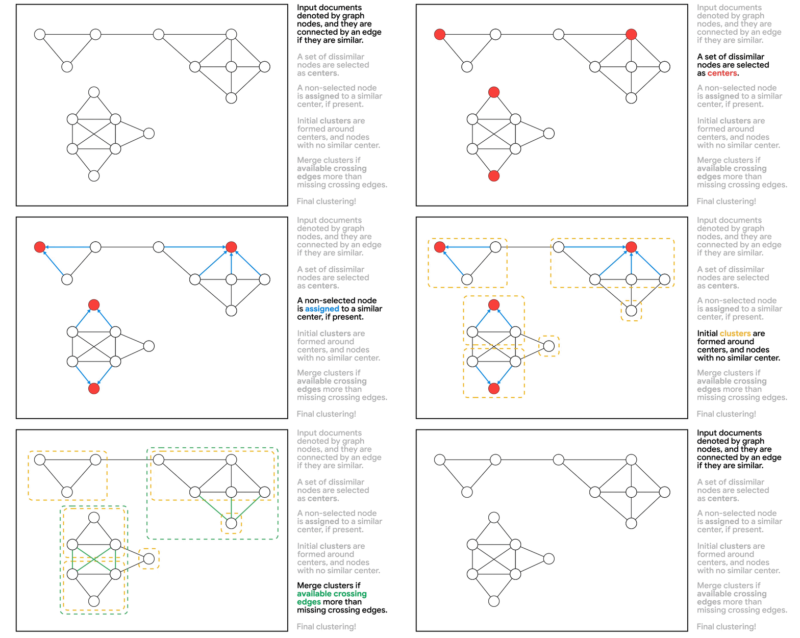
The KwikBucks algorithm is an extension of the well-known KwikCluster algorithm (Pivot algorithm). The high-level idea is to first select a set of documents (i.e., centers) with no similarity edge between them, and then form clusters around these centers. To obtain the quality from CA models and the runtime efficiency from embedding models, we introduce the novel combo similarity oracle mechanism. In this approach, we utilize the embedding model to guide the selection of queries to be sent to the CA model. When given a set of center documents and a target document, the combo similarity oracle mechanism outputs a center from the set that is similar to the target document, if present. The combo similarity oracle enables us to save on budget by limiting the number of query calls to the CA model when selecting centers and forming clusters. It does this by first ranking centers based on their embedding similarity to the target document, and then querying the CA model for the pair (i.e., target document and ranked center), as shown below.

A combo similarity oracle that for a set of documents and a target document, returns a similar document from the set, if present.

We then perform a post processing step to merge clusters if there is a strong connection between two of them, i.e., when the number of connecting edges is higher than the number of missing edges between two clusters. Additionally, we apply the following steps for further computational savings on queries made to the CA model, and to improve performance at runtime:

  1. We leverage query-efficient correlation clustering to form a set of centers from a set of randomly selected documents instead of selecting these centers from all the documents (in the illustration below, the center nodes are red).
  2. We apply the combo similarity oracle mechanism to perform the cluster assignment step in parallel for all non-center documents and leave documents with no similar center as singletons. In the illustration below, the assignments are depicted by blue arrows and initially two (non-center) nodes are left as singletons due to no assignment.
  3. In the post-processing step, to ensure scalability, we use the embedding similarity scores to filter down the potential mergers (in the illustration below, the green dashed boundaries show these merged clusters).

Illustration of progress of the clustering algorithm on a given graph instance.


Results

We evaluate the novel clustering algorithm on various datasets with different properties using different embedding-based and cross-attention–based models. We compare the clustering algorithm’s performance with the two best performing baselines (see the paper for more details):

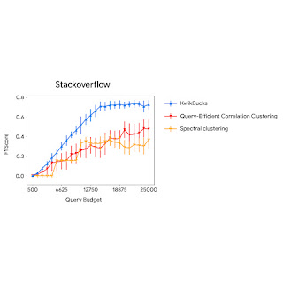
To evaluate the quality of clustering, we use precision and recall. Precision is used to calculate the percentage of similar pairs out of all co-clustered pairs and recall is the percentage of co-clustered similar pairs out of all similar pairs. To measure the quality of the obtained solutions from our experiments, we use the F1-score, which is the harmonic mean of the precision and recall, where 1.0 is the highest possible value that indicates perfect precision and recall, and 0 is the lowest possible value that indicates if either precision or recall are zero. The table below reports the F1-score for Kwikbucks and various baselines in the case that we allow only a linear number of queries to the CA model. We show that Kwikbucks offers a substantial boost in performance with a 45% relative improvement compared to the best baseline when averaging across all datasets.

Comparing the clustering algorithm to two baseline algorithms using various public datasets: (1) The query-efficient correlation clustering algorithm for budgeted clustering with access to CA only, and (2) spectral clustering on the k-nearest neighbor (kNN) graph formed by querying the CA model for the k-nearest neighbors of each vertex from embedding-based similarity. Pre-processed datasets can be downloaded here.

The figure below compares the clustering algorithm’s performance with baselines using different query budgets. We observe that KwikBucks consistently outperforms other baselines at various budgets.

A comparison of KwikBucks with top-2 baselines when allowed different budgets for querying the cross-attention model.


Conclusion

Text clustering often presents a dilemma in the choice of similarity function: embedding models are scalable but lack quality, while cross-attention models offer quality but substantially hurt scalability. We present a clustering algorithm that offers the best of both worlds: the scalability of embedding models and the quality of cross-attention models. KwikBucks can also be applied to other clustering problems with multiple similarity oracles of varying accuracy levels. This is validated with an exhaustive set of experiments on various datasets with diverse properties. See the paper for more details.


Acknowledgements

This project was initiated during Sandeep Silwal’s summer internship at Google in 2022. We would like to express our gratitude to our co-authors, Andrew McCallum, Andrew Nystrom, Deepak Ramachandran, and Sandeep Silwal, for their valuable contributions to this work. We also thank Ravi Kumar and John Guilyard for assistance with this blog post.

Source: Google AI Blog


A novel computational fluid dynamics framework for turbulent flow research

Turbulence is ubiquitous in environmental and engineering fluid flows, and is encountered routinely in everyday life. A better understanding of these turbulent processes could provide valuable insights across a variety of research areas — improving the prediction of cloud formation by atmospheric transport and the spreading of wildfires by turbulent energy exchange, understanding sedimentation of deposits in rivers, and improving the efficiency of combustion in aircraft engines to reduce emissions, to name a few. However, despite its importance, our current understanding and our ability to reliably predict such flows remains limited. This is mainly attributed to the highly chaotic nature and the enormous spatial and temporal scales these fluid flows occupy, ranging from energetic, large-scale movements on the order of several meters on the high-end, where energy is injected into the fluid flow, all the way down to micrometers (μm) on the low-end, where the turbulence is dissipated into heat by viscous friction.

A powerful tool to understand these turbulent flows is the direct numerical simulation (DNS), which provides a detailed representation of the unsteady three-dimensional flow-field without making any approximations or simplifications. More specifically, this approach utilizes a discrete grid with small enough grid spacing to capture the underlying continuous equations that govern the dynamics of the system (in this case, variable-density Navier-Stokes equations, which govern all fluid flow dynamics). When the grid spacing is small enough, the discrete grid points are enough to represent the true (continuous) equations without the loss of accuracy. While this is attractive, such simulations require tremendous computational resources in order to capture the correct fluid-flow behaviors across such a wide range of spatial scales.

The actual span in spatial resolution to which direct numerical calculations must be applied depends on the task and is determined by the Reynolds number, which compares inertial to viscous forces. Typically, the Reynolds number can range between 102 up to 107 (even larger for atmospheric or interstellar problems). In 3D, the grid size for the resolution required scales roughly with the Reynolds number to the power of 4.5! Because of this strong scaling dependency, simulating such flows is generally limited to flow regimes with moderate Reynolds numbers, and typically requires access to high-performance computing systems with millions of CPU/GPU cores.

In “A TensorFlow simulation framework for scientific computing of fluid flows on tensor processing units”, we introduce a new simulation framework that enables the computation of fluid flows with TPUs. By leveraging latest advances on TensorFlow software and TPU-hardware architecture, this software tool allows detailed large-scale simulations of turbulent flows at unprecedented scale, pushing the boundaries of scientific discovery and turbulence analysis. We demonstrate that this framework scales efficiently to accommodate the scale of the problem or, alternatively, improved run times, which is remarkable since most large-scale distributed computation frameworks exhibit reduced efficiency with scaling. The software is available as an open-source project on GitHub.


Large-scale scientific computation with accelerators

The software solves variable-density Navier-Stokes equations on TPU architectures using the TensorFlow framework. The single-instruction, multiple-data (SIMD) approach is adopted for parallelization of the TPU solver implementation. The finite difference operators on a colocated structured mesh are cast as filters of the convolution function of TensorFlow, leveraging TPU’s matrix multiply unit (MXU). The framework takes advantage of the low-latency high-bandwidth inter-chips interconnect (ICI) between the TPU accelerators. In addition, by leveraging the single-precision floating-point computations and highly optimized executable through the accelerated linear algebra (XLA) compiler, it’s possible to perform large-scale simulations with excellent scaling on TPU hardware architectures.

This research effort demonstrates that the graph-based TensorFlow in combination with new types of ML special purpose hardware, can be used as a programming paradigm to solve partial differential equations representing multiphysics flows. The latter is achieved by augmenting the Navier-Stokes equations with physical models to account for chemical reactions, heat-transfer, and density changes to enable, for example, simulations of cloud formation and wildfires.

It’s worth noting that this framework is the first open-source computational fluid dynamics (CFD) framework for high-performance, large-scale simulations to fully leverage the cloud accelerators that have become common (and become a commodity) with the advancement of machine learning (ML) in recent years. While our work focuses on using TPU accelerators, the code can be easily adjusted for other accelerators, such as GPU clusters.

This framework demonstrates a way to greatly reduce the cost and turn-around time associated with running large-scale scientific CFD simulations and enables even greater iteration speed in fields, such as climate and weather research. Since the framework is implemented using TensorFlow, an ML language, it also enables the ready integration with ML methods and allows the exploration of ML approaches on CFD problems. With the general accessibility of TPU and GPU hardware, this approach lowers the barrier for researchers to contribute to our understanding of large-scale turbulent systems.


Framework validation and homogeneous isotropic turbulence

Beyond demonstrating the performance and the scaling capabilities, it is also critical to validate the correctness of this framework to ensure that when it is used for CFD problems, we get reasonable results. For this purpose, researchers typically use idealized benchmark problems during CFD solver development, many of which we adopted in our work (more details in the paper).

One such benchmark for turbulence analysis is homogeneous isotropic turbulence (HIT), which is a canonical and well studied flow in which the statistical properties, such as kinetic energy, are invariant under translations and rotations of the coordinate axes. By pushing the resolution to the limits of the current state of the art, we were able to perform direct numerical simulations with more than eight billion degrees of freedom — equivalent to a three-dimensional mesh with 2,048 grid points along each of the three directions. We used 512 TPU-v4 cores, distributing the computation of the grid points along the x, y, and z axes to a distribution of [2,2,128] cores, respectively, optimized for the performance on TPU. The wall clock time per timestep was around 425 milliseconds and the flow was simulated for a total of 400,000 timesteps. 50 TB data, which includes the velocity and density fields, is stored for 400 timesteps (every 1,000th step). To our knowledge, this is one of the largest turbulent flow simulations of its kind conducted to date.

Due to the complex, chaotic nature of the turbulent flow field, which extends across several magnitudes of resolution, simulating the system in high resolution is necessary. Because we employ a fine-resolution grid with eight billion points, we are able to accurately resolve the field.

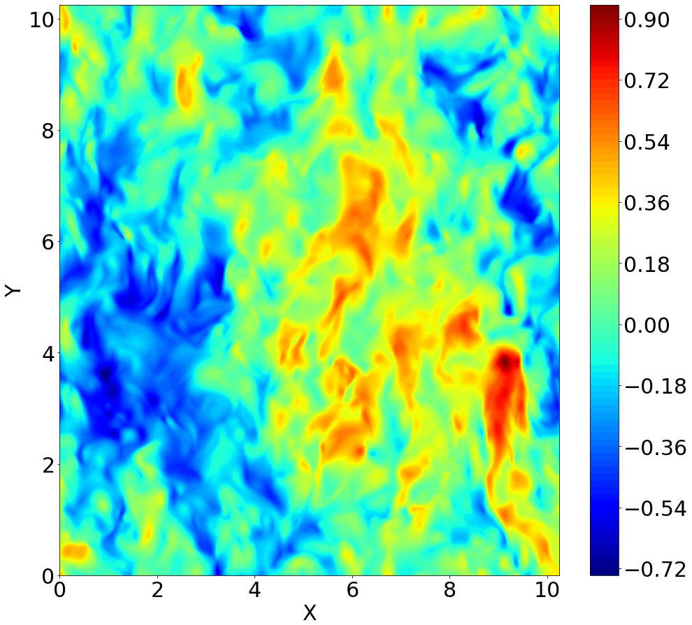
Contours of x-component of velocity along the z midplane. The high resolution of the simulation is critical to accurately represent the turbulent field.

The turbulent kinetic energy and dissipation rates are two statistical quantities commonly used to analyze a turbulent flow. The temporal decay of these properties in a turbulent field without additional energy injection is due to viscous dissipation and the decay asymptotes follow the expected analytical power law. This is in agreement with the theoretical asymptotes and observations reported in the literature and thus, validates our framework.

Solid line: Temporal evolution of turbulent kinetic energy (k). Dashed line: Analytical power laws for decaying homogeneous isotropic turbulence (n=1.3) (l: eddy turnover time).
Solid line: Temporal evolution of dissipation rate (ε). Dashed line: Analytical power laws for decaying homogeneous isotropic turbulence (n=1.3).

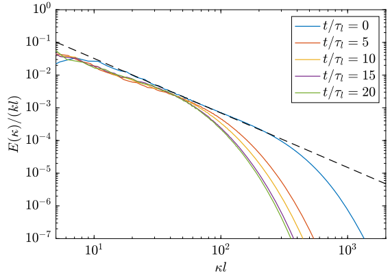
The energy spectrum of a turbulent flow represents the energy content across wavenumber, where the wavenumber k is proportional to the inverse wavelength λ (i.e., k ∝ 1/λ). Generally, the spectrum can be qualitatively divided into three ranges: source range, inertial range and viscous dissipative range (from left to right on the wavenumber axis, below). The lowest wavenumbers in the source range correspond to the largest turbulent eddies, which have the most energy content. These large eddies transfer energy to turbulence in the intermediate wavenumbers (inertial range), which is statistically isotropic (i.e., essentially uniform in all directions). The smallest eddies, corresponding to the largest wavenumbers, are dissipated into thermal energy by the viscosity of the fluid. By virtue of the fine grid having 2,048 points in each of the three spatial directions, we are able to resolve the flow field up to the length scale at which viscous dissipation takes place. This direct numerical simulation approach is the most accurate as it does not require any closure model to approximate the energy cascade below the grid size.

Spectrum of turbulent kinetic energy at different time instances. The spectrum is normalized by the instantaneous integral length (l) and the turbulent kinetic energy (k).

A new era for turbulent flows research

More recently, we extended this framework to predict wildfires and atmospheric flows, which is relevant for climate-risk assessment. Apart from enabling high-fidelity simulations of complex turbulent flows, this simulation framework also provides capabilities for scientific machine learning (SciML) — for example, downsampling from a fine to a coarse grid (model reduction) or building models that run at lower resolution while still capturing the correct dynamic behaviors. It could also provide avenues for further scientific discovery, such as building ML-based models to better parameterize microphysics of turbulent flows, including physical relationships between temperature, pressure, vapor fraction, etc., and could improve upon various control tasks, e.g., to reduce the energy consumption of buildings or find more efficient propeller shapes. While attractive, a main bottleneck in SciML has been the availability of data for training. To explore this, we have been working with groups at Stanford and Kaggle to make the data from our high-resolution HIT simulation available through a community-hosted web-platform, BLASTNet, to provide broad access to high-fidelity data to the research community via a network-of-datasets approach. We hope that the availability of these emerging high-fidelity simulation tools in conjunction with community-driven datasets will lead to significant advances in various areas of fluid mechanics.


Acknowledgements

We would like to thank Qing Wang, Yi-Fan Chen, and John Anderson for consulting and advice, Tyler Russell and Carla Bromberg for program management.

Source: Google AI Blog


AdaTape: Foundation model with adaptive computation and dynamic read-and-write

Adaptive computation refers to the ability of a machine learning system to adjust its behavior in response to changes in the environment. While conventional neural networks have a fixed function and computation capacity, i.e., they spend the same number of FLOPs for processing different inputs, a model with adaptive and dynamic computation modulates the computational budget it dedicates to processing each input, depending on the complexity of the input.

Adaptive computation in neural networks is appealing for two key reasons. First, the mechanism that introduces adaptivity provides an inductive bias that can play a key role in solving some challenging tasks. For instance, enabling different numbers of computational steps for different inputs can be crucial in solving arithmetic problems that require modeling hierarchies of different depths. Second, it gives practitioners the ability to tune the cost of inference through greater flexibility offered by dynamic computation, as these models can be adjusted to spend more FLOPs processing a new input.

Neural networks can be made adaptive by using different functions or computation budgets for various inputs. A deep neural network can be thought of as a function that outputs a result based on both the input and its parameters. To implement adaptive function types, a subset of parameters are selectively activated based on the input, a process referred to as conditional computation. Adaptivity based on the function type has been explored in studies on mixture-of-experts, where the sparsely activated parameters for each input sample are determined through routing.

Another area of research in adaptive computation involves dynamic computation budgets. Unlike in standard neural networks, such as T5, GPT-3, PaLM, and ViT, whose computation budget is fixed for different samples, recent research has demonstrated that adaptive computation budgets can improve performance on tasks where transformers fall short. Many of these works achieve adaptivity by using dynamic depth to allocate the computation budget. For example, the Adaptive Computation Time (ACT) algorithm was proposed to provide an adaptive computational budget for recurrent neural networks. The Universal Transformer extends the ACT algorithm to transformers by making the computation budget dependent on the number of transformer layers used for each input example or token. Recent studies, like PonderNet, follow a similar approach while improving the dynamic halting mechanisms.

In the paper “Adaptive Computation with Elastic Input Sequence”, we introduce a new model that utilizes adaptive computation, called AdaTape. This model is a Transformer-based architecture that uses a dynamic set of tokens to create elastic input sequences, providing a unique perspective on adaptivity in comparison to previous works. AdaTape uses an adaptive tape reading mechanism to determine a varying number of tape tokens that are added to each input based on input’s complexity. AdaTape is very simple to implement, provides an effective knob to increase the accuracy when needed, but is also much more efficient compared to other adaptive baselines because it directly injects adaptivity into the input sequence instead of the model depth. Finally, Adatape offers better performance on standard tasks, like image classification, as well as algorithmic tasks, while maintaining a favorable quality and cost tradeoff.


Adaptive computation transformer with elastic input sequence

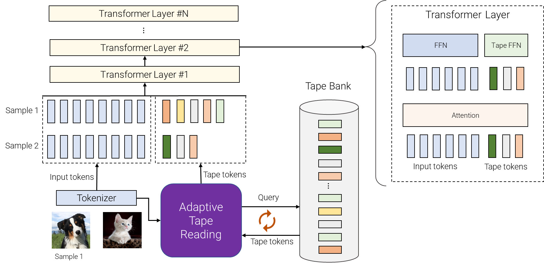
AdaTape uses both the adaptive function types and a dynamic computation budget. Specifically, for a batch of input sequences after tokenization (e.g., a linear projection of non-overlapping patches from an image in the vision transformer), AdaTape uses a vector representing each input to dynamically select a variable-sized sequence of tape tokens.

AdaTape uses a bank of tokens, called a “tape bank”, to store all the candidate tape tokens that interact with the model through the adaptive tape reading mechanism. We explore two different methods for creating the tape bank: an input-driven bank and a learnable bank.

The general idea of the input-driven bank is to extract a bank of tokens from the input while employing a different approach than the original model tokenizer for mapping the raw input to a sequence of input tokens. This enables dynamic, on-demand access to information from the input that is obtained using a different point of view, e.g., a different image resolution or a different level of abstraction.

In some cases, tokenization in a different level of abstraction is not possible, thus an input-driven tape bank is not feasible, such as when it's difficult to further split each node in a graph transformer. To address this issue, AdaTape offers a more general approach for generating the tape bank by using a set of trainable vectors as tape tokens. This approach is referred to as the learnable bank and can be viewed as an embedding layer where the model can dynamically retrieve tokens based on the complexity of the input example. The learnable bank enables AdaTape to generate a more flexible tape bank, providing it with the ability to dynamically adjust its computation budget based on the complexity of each input example, e.g., more complex examples retrieve more tokens from the bank, which let the model not only use the knowledge stored in the bank, but also spend more FLOPs processing it, since the input is now larger.

Finally, the selected tape tokens are appended to the original input and fed to the following transformer layers. For each transformer layer, the same multi-head attention is used across all input and tape tokens. However, two different feed-forward networks (FFN) are used: one for all tokens from the original input and the other for all tape tokens. We observed slightly better quality by using separate feed-forward networks for input and tape tokens.

An overview of AdaTape. For different samples, we pick a variable number of different tokens from the tape bank. The tape bank can be driven from input, e.g., by extracting some extra fine-grained information or it can be a set of trainable vectors. Adaptive tape reading is used to recursively select different sequences of tape tokens, with variable lengths, for different inputs. These tokens are then simply appended to inputs and fed to the transformer encoder.

AdaTape provides helpful inductive bias

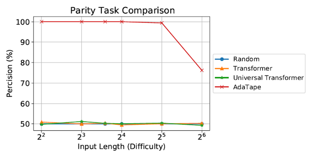
We evaluate AdaTape on parity, a very challenging task for the standard Transformer, to study the effect of inductive biases in AdaTape. With the parity task, given a sequence 1s, 0s, and -1s, the model has to predict the evenness or oddness of the number of 1s in the sequence. Parity is the simplest non-counter-free or periodic regular language, but perhaps surprisingly, the task is unsolvable by the standard Transformer.

Evaluation on the parity task. The standard Transformer and Universal Transformer were unable to perform this task, both showing performance at the level of a random guessing baseline.

Despite being evaluated on short, simple sequences, both the standard Transformer and Universal Transformers were unable to perform the parity task as they are unable to maintain a counter within the model. However, AdaTape outperforms all baselines, as it incorporates a lightweight recurrence within its input selection mechanism, providing an inductive bias that enables the implicit maintenance of a counter, which is not possible in standard Transformers.


Evaluation on image classification

We also evaluate AdaTape on the image classification task. To do so, we trained AdaTape on ImageNet-1K from scratch. The figure below shows the accuracy of AdaTape and the baseline methods, including A-ViT, and the Universal Transformer ViT (UViT and U2T) versus their speed (measured as number of images, processed by each code, per second). In terms of quality and cost tradeoff, AdaTape performs much better than the alternative adaptive transformer baselines. In terms of efficiency, larger AdaTape models (in terms of parameter count) are faster than smaller baselines. Such results are consistent with the finding from previous work that shows that the adaptive model depth architectures are not well suited for many accelerators, like the TPU.

We evaluate AdaTape by training on ImageNet from scratch. For A-ViT, we not only report their results from the paper but also re-implement A-ViT by training from scratch, i.e., A-ViT(Ours).

A study of AdaTape’s behavior

In addition to its performance on the parity task and ImageNet-1K, we also evaluated the token selection behavior of AdaTape with an input-driven bank on the JFT-300M validation set. To better understand the model's behavior, we visualized the token selection results on the input-driven bank as heatmaps, where lighter colors mean that position is more frequently selected. The heatmaps reveal that AdaTape more frequently picks the central patches. This aligns with our prior knowledge, as central patches are typically more informative — especially in the context of datasets with natural images, where the main object is in the middle of the image. This result highlights the intelligence of AdaTape, as it can effectively identify and prioritize more informative patches to improve its performance.

We visualize the tape token selection heatmap of AdaTape-B/32 (left) and AdaTape-B/16 (right). The hotter / lighter color means the patch at this position is more frequently selected.

Conclusion

AdaTape is characterized by elastic sequence lengths generated by the adaptive tape reading mechanism. This also introduces a new inductive bias that enables AdaTape to have the potential to solve tasks that are challenging for both standard transformers and existing adaptive transformers. By conducting comprehensive experiments on image recognition benchmarks, we demonstrate that AdaTape outperforms standard transformers and adaptive architecture transformers when computation is held constant.


Acknowledgments

One of the authors of this post, Mostafa Dehghani, is now at Google DeepMind.

Source: Google AI Blog


Differentially private heatmaps

Recently, differential privacy (DP) has emerged as a mathematically robust notion of user privacy for data aggregation and machine learning (ML), with practical deployments including the 2022 US Census and in industry. Over the last few years, we have open-sourced libraries for privacy-preserving analytics and ML and have been constantly enhancing their capabilities. Meanwhile, new algorithms have been developed by the research community for several analytic tasks involving private aggregation of data.

One such important data aggregation method is the heatmap. Heatmaps are popular for visualizing aggregated data in two or more dimensions. They are widely used in many fields including computer vision, image processing, spatial data analysis, bioinformatics, and more. Protecting the privacy of user data is critical for many applications of heatmaps. For example, heatmaps for gene microdata are based on private data from individuals. Similarly, a heatmap of popular locations in a geographic area are based on user location check-ins that need to be kept private.

Motivated by such applications, in “Differentially Private Heatmaps” (presented at AAAI 2023), we describe an efficient DP algorithm for computing heatmaps with provable guarantees and evaluate it empirically. At the core of our DP algorithm for heatmaps is a solution to the basic problem of how to privately aggregate sparse input vectors (i.e., input vectors with a small number of non-zero coordinates) with a small error as measured by the Earth Mover's Distance (EMD). Using a hierarchical partitioning procedure, our algorithm views each input vector, as well as the output heatmap, as a probability distribution over a number of items equal to the dimension of the data. For the problem of sparse aggregation under EMD, we give an efficient algorithm with error asymptotically close to the best possible.


Algorithm description

Our algorithm works by privatizing the aggregated distribution (obtained by averaging over all user inputs), which is sufficient for computing a final heatmap that is private due to the post-processing property of DP. This property ensures that any transformation of the output of a DP algorithm remains differentially private. Our main contribution is a new privatization algorithm for the aggregated distribution, which we will describe next.

The EMD measure, which is a distance-like measure of dissimilarity between two probability distributions originally proposed for computer vision tasks, is well-suited for heatmaps since it takes the underlying metric space into account and considers "neighboring" bins. EMD is used in a variety of applications including deep learning, spatial analysis, human mobility, image retrieval, face recognition, visual tracking, shape matching, and more.

To achieve DP, we need to add noise to the aggregated distribution. We would also like to preserve statistics at different scales of the grid to minimize the EMD error. So, we create a hierarchical partitioning of the grid, add noise at each level, and then recombine into the final DP aggregated distribution. In particular, the algorithm has the following steps:

  1. Quadtree construction: Our hierarchical partitioning procedure first divides the grid into four cells, then divides each cell into four subcells; it recursively continues this process until each cell is a single pixel. This procedure creates a quadtree over the subcells where the root represents the entire grid and each leaf represents a pixel. The algorithm then calculates the total probability mass for each tree node (obtained by adding up the aggregated distribution’s probabilities of all leaves in the subtree rooted at this node). This step is illustrated below.
    In the first step, we take the (non-private) aggregated distribution (top left) and repeatedly divide it to create a quadtree. Then, we compute the total probability mass is each cell (bottom).
  2. Noise addition: To each tree node’s mass we then add Laplace noise calibrated to the use case.
  3. Truncation: To help reduce the final amount of noise in our DP aggregated distribution, the algorithm traverses the tree starting from the root and, at each level, it discards all but the top w nodes with highest (noisy) masses together with their descendants.
  4. Reconstruction: Finally, the algorithm solves a linear program to recover the aggregated distribution. This linear program is inspired by the sparse recovery literature where the noisy masses are viewed as (noisy) measurements of the data.
In step 2, noise is added to each cell’s probability mass. Then in step 3, only top-w cells are kept (green) whereas the remaining cells are truncated (red). Finally, in the last step, we write a linear program on these top cells to reconstruct the aggregation distribution, which is now differentially private.

Experimental results

We evaluate the performance of our algorithm in two different domains: real-world location check-in data and image saliency data. We consider as a baseline the ubiquitous Laplace mechanism, where we add Laplace noise to each cell, zero out any negative cells, and produce the heatmap from this noisy aggregate. We also consider a “thresholding” variant of this baseline that is more suited to sparse data: only keep top t% of the cell values (based on the probability mass in each cell) after noising while zeroing out the rest. To evaluate the quality of an output heatmap compared to the true heatmap, we use Pearson coefficient, KL-divergence, and EMD. Note that when the heatmaps are more similar, the first metric increases but the latter two decrease.

The locations dataset is obtained by combining two datasets, Gowalla and Brightkite, both of which contain check-ins by users of location-based social networks. We pre-processed this dataset to consider only check-ins in the continental US resulting in a final dataset consisting of ~500,000 check-ins by ~20,000 users. Considering the top cells (from an initial partitioning of the entire space into a 300 x 300 grid) that have check-ins from at least 200 unique users, we partition each such cell into subgrids with a resolution of ∆ × ∆ and assign each check-in to one of these subgrids.

In the first set of experiments, we fix ∆ = 256. We test the performance of our algorithm for different values of ε (the privacy parameter, where smaller ε means stronger DP guarantees), ranging from 0.1 to 10, by running our algorithms together with the baseline and its variants on all cells, randomly sampling a set of 200 users in each trial, and then computing the distance metrics between the true heatmap and the DP heatmap. The average of these metrics is presented below. Our algorithm (the red line) performs better than all versions of the baseline across all metrics, with improvements that are especially significant when ε is not too large or small (i.e., 0.2 ≤ ε ≤ 5).

Metrics averaged over 60 runs when varying ε for the location dataset. Shaded areas indicate 95% confidence interval.

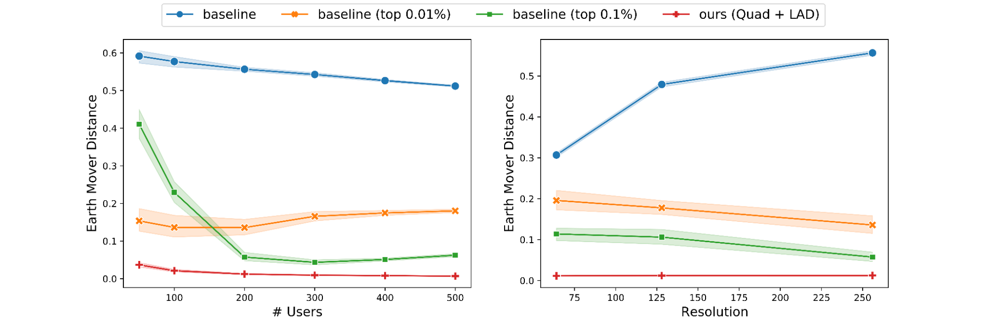
Next, we study the effect of varying the number n of users. By fixing a single cell (with > 500 users) and ε, we vary n from 50 to 500 users. As predicted by theory, our algorithms and the baseline perform better as n increases. However, the behavior of the thresholding variants of the baseline are less predictable.

We also run another experiment where we fix a single cell and ε, and vary the resolution ∆ from 64 to 256. In agreement with theory, our algorithm’s performance remains nearly constant for the entire range of ∆. However, the baseline suffers across all metrics as ∆ increases while the thresholding variants occasionally improve as ∆ increases.

Effect of the number of users and grid resolution on EMD.

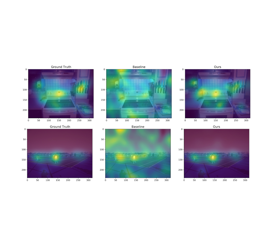
We also experiment on the Salicon image saliency dataset (SALICON). This dataset is a collection of saliency annotations on the Microsoft Common Objects in Context image database. We downsized the images to a fixed resolution of 320 × 240 and each [user, image] pair consists of a sequence of coordinates in the image where the user looked. We repeat the experiments described previously on 38 randomly sampled images (with ≥ 50 users each) from SALICON. As we can see from the examples below, the heatmap obtained by our algorithm is very close to the ground truth.

Example visualization of different algorithms for two different natural images from SALICON for ε = 10 and n = 50 users. The algorithms from left to right are: original heatmap (no privacy), baseline, and ours.

Additional experimental results, including those on other datasets, metrics, privacy parameters and DP models, can be found in the paper.


Conclusion

We presented a privatization algorithm for sparse distribution aggregation under the EMD metric, which in turn yields an algorithm for producing privacy-preserving heatmaps. Our algorithm extends naturally to distributed models that can implement the Laplace mechanism, including the secure aggregation model and the shuffle model. This does not apply to the more stringent local DP model, and it remains an interesting open question to devise practical local DP heatmap/EMD aggregation algorithms for “moderate” number of users and privacy parameters.


Acknowledgments

This work was done jointly with Junfeng He, Kai Kohlhoff, Ravi Kumar, Pasin Manurangsi, and Vidhya Navalpakkam.

Source: Google AI Blog


Beyond automatic differentiation

Derivatives play a central role in optimization and machine learning. By locally approximating a training loss, derivatives guide an optimizer toward lower values of the loss. Automatic differentiation frameworks such as TensorFlow, PyTorch, and JAX are an essential part of modern machine learning, making it feasible to use gradient-based optimizers to train very complex models.

But are derivatives all we need? By themselves, derivatives only tell us how a function behaves on an infinitesimal scale. To use derivatives effectively, we often need to know more than that. For example, to choose a learning rate for gradient descent, we need to know something about how the loss function behaves over a small but finite window. A finite-scale analogue of automatic differentiation, if it existed, could help us make such choices more effectively and thereby speed up training.

In our new paper "Automatically Bounding The Taylor Remainder Series: Tighter Bounds and New Applications", we present an algorithm called AutoBound that computes polynomial upper and lower bounds on a given function, which are valid over a user-specified interval. We then begin to explore AutoBound's applications. Notably, we present a meta-optimizer called SafeRate that uses the upper bounds computed by AutoBound to derive learning rates that are guaranteed to monotonically reduce a given loss function, without the need for time-consuming hyperparameter tuning. We are also making AutoBound available as an open-source library.


The AutoBound algorithm

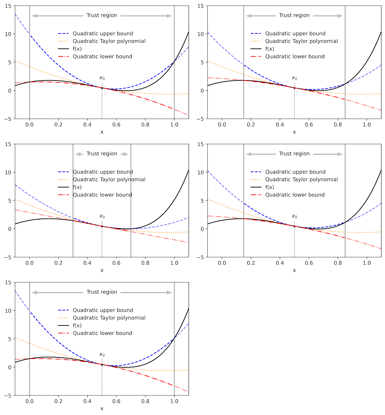
Given a function f and a reference point x0, AutoBound computes polynomial upper and lower bounds on f that hold over a user-specified interval called a trust region. Like Taylor polynomials, the bounding polynomials are equal to f at x0. The bounds become tighter as the trust region shrinks, and approach the corresponding Taylor polynomial as the trust region width approaches zero.

Automatically-derived quadratic upper and lower bounds on a one-dimensional function f, centered at x0=0.5. The upper and lower bounds are valid over a user-specified trust region, and become tighter as the trust region shrinks.

Like automatic differentiation, AutoBound can be applied to any function that can be implemented using standard mathematical operations. In fact, AutoBound is a generalization of Taylor mode automatic differentiation, and is equivalent to it in the special case where the trust region has a width of zero.

To derive the AutoBound algorithm, there were two main challenges we had to address:

  1. We had to derive polynomial upper and lower bounds for various elementary functions, given an arbitrary reference point and arbitrary trust region.
  2. We had to come up with an analogue of the chain rule for combining these bounds.

Bounds for elementary functions

For a variety of commonly-used functions, we derive optimal polynomial upper and lower bounds in closed form. In this context, "optimal" means the bounds are as tight as possible, among all polynomials where only the maximum-degree coefficient differs from the Taylor series. Our theory applies to elementary functions, such as exp and log, and common neural network activation functions, such as ReLU and Swish. It builds upon and generalizes earlier work that applied only to quadratic bounds, and only for an unbounded trust region.

Optimal quadratic upper and lower bounds on the exponential function, centered at x0=0.5 and valid over the interval [0, 2].

A new chain rule

To compute upper and lower bounds for arbitrary functions, we derived a generalization of the chain rule that operates on polynomial bounds. To illustrate the idea, suppose we have a function that can be written as

f(x) = g(h(x))

and suppose we already have polynomial upper and lower bounds on g and h. How do we compute bounds on f?

The key turns out to be representing the upper and lower bounds for a given function as a single polynomial whose highest-degree coefficient is an interval rather than a scalar. We can then plug the bound for h into the bound for g, and convert the result back to a polynomial of the same form using interval arithmetic. Under suitable assumptions about the trust region over which the bound on g holds, it can be shown that this procedure yields the desired bound on f.

The interval polynomial chain rule applied to the functions h(x) = sqrt(x) and g(y) = exp(y), with x0=0.25 and trust region [0, 0.5].

Our chain rule applies to one-dimensional functions, but also to multivariate functions, such as matrix multiplications and convolutions.


Propagating bounds

Using our new chain rule, AutoBound propagates interval polynomial bounds through a computation graph from the inputs to the outputs, analogous to forward-mode automatic differentiation.

Forward propagation of interval polynomial bounds for the function f(x) = exp(sqrt(x)). We first compute (trivial) bounds on x, then use the chain rule to compute bounds on sqrt(x) and exp(sqrt(x)).

To compute bounds on a function f(x), AutoBound requires memory proportional to the dimension of x. For this reason, practical applications apply AutoBound to functions with a small number of inputs. However, as we will see, this does not prevent us from using AutoBound for neural network optimization.


Automatically deriving optimizers, and other applications

What can we do with AutoBound that we couldn't do with automatic differentiation alone?

Among other things, AutoBound can be used to automatically derive problem-specific, hyperparameter-free optimizers that converge from any starting point. These optimizers iteratively reduce a loss by first using AutoBound to compute an upper bound on the loss that is tight at the current point, and then minimizing the upper bound to obtain the next point.

Minimizing a one-dimensional logistic regression loss using quadratic upper bounds derived automatically by AutoBound.

Optimizers that use upper bounds in this way are called majorization-minimization (MM) optimizers. Applied to one-dimensional logistic regression, AutoBound rederives an MM optimizer first published in 2009. Applied to more complex problems, AutoBound derives novel MM optimizers that would be difficult to derive by hand.

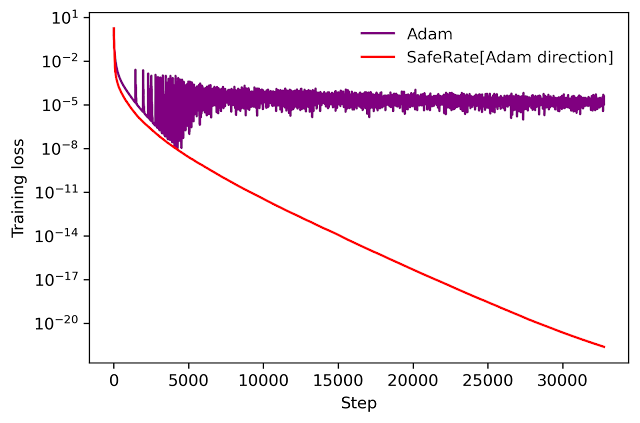
We can use a similar idea to take an existing optimizer such as Adam and convert it to a hyperparameter-free optimizer that is guaranteed to monotonically reduce the loss (in the full-batch setting). The resulting optimizer uses the same update direction as the original optimizer, but modifies the learning rate by minimizing a one-dimensional quadratic upper bound derived by AutoBound. We refer to the resulting meta-optimizer as SafeRate.

Performance of SafeRate when used to train a single-hidden-layer neural network on a subset of the MNIST dataset, in the full-batch setting.

Using SafeRate, we can create more robust variants of existing optimizers, at the cost of a single additional forward pass that increases the wall time for each step by a small factor (about 2x in the example above).

In addition to the applications just discussed, AutoBound can be used for verified numerical integration and to automatically prove sharper versions of Jensen's inequality, a fundamental mathematical inequality used frequently in statistics and other fields.


Improvement over classical bounds

Bounding the Taylor remainder term automatically is not a new idea. A classical technique produces degree k polynomial bounds on a function f that are valid over a trust region [a, b] by first computing an expression for the kth derivative of f (using automatic differentiation), then evaluating this expression over [a,b] using interval arithmetic.

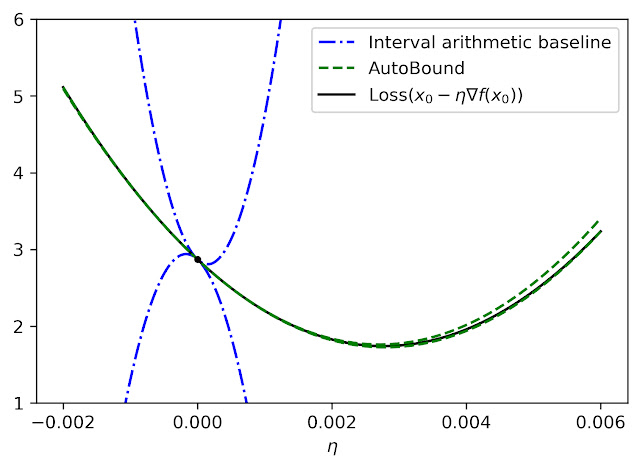
While elegant, this approach has some inherent limitations that can lead to very loose bounds, as illustrated by the dotted blue lines in the figure below.

Quadratic upper and lower bounds on the loss of a multi-layer perceptron with two hidden layers, as a function of the initial learning rate. The bounds derived by AutoBound are much tighter than those obtained using interval arithmetic evaluation of the second derivative.

Looking forward

Taylor polynomials have been in use for over three hundred years, and are omnipresent in numerical optimization and scientific computing. Nevertheless, Taylor polynomials have significant limitations, which can limit the capabilities of algorithms built on top of them. Our work is part of a growing literature that recognizes these limitations and seeks to develop a new foundation upon which more robust algorithms can be built.

Our experiments so far have only scratched the surface of what is possible using AutoBound, and we believe it has many applications we have not discovered. To encourage the research community to explore such possibilities, we have made AutoBound available as an open-source library built on top of JAX. To get started, visit our GitHub repo.


Acknowledgements

This post is based on joint work with Josh Dillon. We thank Alex Alemi and Sergey Ioffe for valuable feedback on an earlier draft of the post.

Source: Google AI Blog


Google Research, 2022 & beyond: Algorithmic advances


(This is Part 5 in our series of posts covering different topical areas of research at Google. You can find other posts in the series here.)

Robust algorithm design is the backbone of systems across Google, particularly for our ML and AI models. Hence, developing algorithms with improved efficiency, performance and speed remains a high priority as it empowers services ranging from Search and Ads to Maps and YouTube. Google Research has been at the forefront of this effort, developing many innovations from privacy-safe recommendation systems to scalable solutions for large-scale ML. In 2022, we continued this journey, and advanced the state-of-the-art in several related areas. Here we highlight our progress in a subset of these, including scalability, privacy, market algorithms, and algorithmic foundations.


Scalable algorithms: Graphs, clustering, and optimization

As the need to handle large-scale datasets increases, scalability and reliability of complex algorithms that also exhibit improved explainability, robustness, and speed remain a high priority. We continued our efforts in developing new algorithms for handling large datasets in various areas, including unsupervised and semi-supervised learning, graph-based learning, clustering, and large-scale optimization.

An important component of such systems is to build a similarity graph — a nearest-neighbor graph that represents similarities between objects. For scalability and speed, this graph should be sparse without compromising quality. We proposed a 2-hop spanner technique, called STAR, as an efficient and distributed graph building strategy, and showed how it significantly decreases the number of similarity computations in theory and practice, building much sparser graphs while producing high-quality graph learning or clustering outputs. As an example, for graphs with 10T edges, we demonstrate ~100-fold improvements in pairwise similarity comparisons and significant running time speedups with negligible quality loss. We had previously applied this idea to develop massively parallel algorithms for metric, and minimum-size clustering. More broadly in the context of clustering, we developed the first linear-time hierarchical agglomerative clustering (HAC) algorithm as well as DBSCAN, the first parallel algorithm for HAC with logarithmic depth, which achieves 50x speedup on 100B-edge graphs. We also designed improved sublinear algorithms for different flavors of clustering problems such as geometric linkage clustering, constant-round correlation clustering, and fully dynamic k-clustering.

Inspired by the success of multi-core processing (e.g., GBBS), we embarked on a mission to develop graph mining algorithms that can handle graphs with 100B edges on a single multi-core machine. The big challenge here is to achieve fast (e.g., sublinear) parallel running time (i.e., depth). Following our previous work for community detection and correlation clustering, we developed an algorithm for HAC, called ParHAC, which has provable polylogarithmic depth and near-linear work and achieves a 50x speedup. As an example, it took ParHAC only ~10 minutes to find an approximate affinity hierarchy over a graph of over 100B edges, and ~3 hours to find the full HAC on a single machine. Following our previous work on distributed HAC, we use these multi-core algorithms as a subroutine within our distributed algorithms in order to handle tera-scale graphs.

We also had a number of interesting results on graph neural networks (GNN) in 2022. We provided a model-based taxonomy that unified many graph learning methods. In addition, we discovered insights for GNN models from their performance across thousands of graphs with varying structure (shown below). We also proposed a new hybrid architecture to overcome the depth requirements of existing GNNs for solving fundamental graph problems, such as shortest paths and the minimum spanning tree.

Relative performance results of three GNN variants (GCN, APPNP, FiLM) across 50,000 distinct node classification datasets in GraphWorld. We find that academic GNN benchmark datasets exist in regions where model rankings do not change. GraphWorld can discover previously unexplored graphs that reveal new insights about GNN architectures.

Furthermore, to bring some of these many advances to the broader community, we had three releases of our flagship modeling library for building graph neural networks in TensorFlow (TF-GNN). Highlights include a model library and model orchestration API to make it easy to compose GNN solutions. Following our NeurIPS’20 workshop on Mining and Learning with Graphs at Scale, we ran a workshop on graph-based learning at ICML’22, and a tutorial for GNNs in TensorFlow at NeurIPS’22.

In “Robust Routing Using Electrical Flows”, we presented a recent paper that proposed a Google Maps solution to efficiently compute alternate paths in road networks that are resistant to failures (e.g., closures, incidents). We demonstrate how it significantly outperforms the state-of-the-art plateau and penalty methods on real-world road networks.

Example of how we construct the electrical circuit corresponding to the road network. The current can be decomposed into three flows, i1, i2 and i3, each of which corresponds to a viable alternate path from Fremont, CA to San Rafael, CA.

On the optimization front, we open-sourced Vizier, our flagship blackbox optimization and hyperparameter tuning library at Google. We also developed new techniques for linear programming (LP) solvers that address scalability limits caused by their reliance on matrix factorizations, which restricts the opportunity for parallelism and distributed approaches. To this end, we open-sourced a primal-dual hybrid gradient (PDHG) solution for LP called primal-dual linear programming (PDLP), a new first-order solver for large-scale LP problems. PDLP has been used to solve real-world problems with as many as 12B non-zeros (and an internal distributed version scaled to 92B non-zeros). PDLP's effectiveness is due to a combination of theoretical developments and algorithm engineering.

With OSS Vizier, multiple clients each send a “Suggest” request to the Service API, which produces Suggestions for the clients using Pythia policies. The clients evaluate these suggestions and return measurements. All transactions are stored to allow fault-tolerance.

Top


Privacy and federated learning

Respecting user privacy while providing high-quality services remains a top priority for all Google systems. Research in this area spans many products and uses principles from differential privacy (DP) and federated learning.

First of all, we have made a variety of algorithmic advances to address the problem of training large neural networks with DP. Building on our earlier work, which enabled us to launch a DP neural network based on the DP-FTRL algorithm, we developed the matrix factorization DP-FTRL approach. This work demonstrates that one can design a mathematical program to optimize over a large set of possible DP mechanisms to find those best suited for specific learning problems. We also establish margin guarantees that are independent of the input feature dimension for DP learning of neural networks and kernel-based methods. We further extend this concept to a broader range of ML tasks, matching baseline performance with 300x less computation. For fine-tuning of large models, we argued that once pre-trained, these models (even with DP) essentially operate over a low-dimensional subspace, hence circumventing the curse of dimensionality that DP imposes.

On the algorithmic front, for estimating the entropy of a high-dimensional distribution, we obtained local DP mechanisms (that work even when as little as one bit per sample is available) and efficient shuffle DP mechanisms. We proposed a more accurate method to simultaneously estimate the top-k most popular items in the database in a private manner, which we employed in the Plume library. Moreover, we showed a near-optimal approximation algorithm for DP clustering in the massively parallel computing (MPC) model, which further improves on our previous work for scalable and distributed settings.

Another exciting research direction is the intersection of privacy and streaming. We obtained a near-optimal approximation-space trade-off for the private frequency moments and a new algorithm for privately counting distinct elements in the sliding window streaming model. We also presented a general hybrid framework for studying adversarial streaming.

Addressing applications at the intersection of security and privacy, we developed new algorithms that are secure, private, and communication-efficient, for measuring cross-publisher reach and frequency. The World Federation of Advertisers has adopted these algorithms as part of their measurement system. In subsequent work, we developed new protocols that are secure and private for computing sparse histograms in the two-server model of DP. These protocols are efficient from both computation and communication points of view, are substantially better than what standard methods would yield, and combine tools and techniques from sketching, cryptography and multiparty computation, and DP.

While we have trained BERT and transformers with DP, understanding training example memorization in large language models (LLMs) is a heuristic way to evaluate their privacy. In particular, we investigated when and why LLMs forget (potentially memorized) training examples during training. Our findings suggest that earlier-seen examples may observe privacy benefits at the expense of examples seen later. We also quantified the degree to which LLMs emit memorized training data.

Top


Market algorithms and causal inference

We also continued our research in improving online marketplaces in 2022. For example, an important recent area in ad auction research is the study of auto-bidding online advertising where the majority of bidding happens via proxy bidders that optimize higher-level objectives on behalf of advertisers. The complex dynamics of users, advertisers, bidders, and ad platforms leads to non-trivial problems in this space. Following our earlier work in analyzing and improving mechanisms under auto-bidding auctions, we continued our research in improving online marketplaces in the context of automation while taking different aspects into consideration, such as user experience and advertiser budgets. Our findings suggest that properly incorporating ML advice and randomization techniques, even in non-truthful auctions, can robustly improve the overall welfare at equilibria among auto-bidding algorithms.

Structure of auto-bidding online ads system.

Beyond auto-bidding systems, we also studied auction improvements in complex environments, e.g., settings where buyers are represented by intermediaries, and with Rich Ads where each ad can be shown in one of several possible variants. We summarize our work in this area in a recent survey. Beyond auctions, we also investigate the use of contracts in multi-agent and adversarial settings.

Online stochastic optimization remains an important part of online advertising systems with application in optimal bidding and budget pacing. Building on our long-term research in online allocation, we recently blogged about dual mirror descent, a new algorithm for online allocation problems that is simple, robust, and flexible. This state-of-the-art algorithm is robust against a wide range of adversarial and stochastic input distributions and can optimize important objectives beyond economic efficiency, such as fairness. We also show that by tailoring dual mirror descent to the special structure of the increasingly popular return-on-spend constraints, we can optimize advertiser value. Dual mirror descent has a wide range of applications and has been used over time to help advertisers obtain more value through better algorithmic decision making.

An overview of the dual mirror descent algorithm.

Furthermore, following our recent work at the interplay of ML, mechanism design and markets, we investigated transformers for asymmetric auction design, designed utility-maximizing strategies for no-regret learning buyers, and developed new learning algorithms to bid or to price in auctions.

An overview of bipartite experimental design to reduce causal interactions between entities.

A critical component of any sophisticated online service is the ability to experimentally measure the response of users and other players to new interventions. A major challenge of estimating these causal effects accurately is handling complex interactions — or interference — between the control and treatment units of these experiments. We combined our graph clustering and causal inference expertise to expand the results of our previous work in this area, with improved results under a flexible response model and a new experimental design that is more effective at reducing these interactions when treatment assignments and metric measurements occur on the same side of a bipartite platform. We also showed how synthetic control and optimization techniques can be combined to design more powerful experiments, especially in small data regimes.

Top


Algorithmic foundations and theory

Finally, we continued our fundamental algorithmic research by tackling long-standing open problems. A surprisingly concise paper affirmatively resolved a four-decade old open question on whether there is a mechanism that guarantees a constant fraction of the gains-from-trade attainable whenever buyer's value weakly exceeds seller's cost. Another recent paper obtained the state-of-the-art approximation for the classic and highly-studied k-means problem. We also improved the best approximation for correlation clustering breaking the barrier approximation factor of 2. Finally, our work on dynamic data structures to solve min-cost and other network flow problems has contributed to a breakthrough line of work in adapting continuous optimization techniques to solve classic discrete optimization problems.

Top


Concluding thoughts

Designing effective algorithms and mechanisms is a critical component of many Google systems that need to handle tera-scale data robustly with critical privacy and safety considerations. Our approach is to develop algorithms with solid theoretical foundations that can be deployed effectively in our product systems. In addition, we are bringing many of these advances to the broader community by open-sourcing some of our most novel developments and by publishing the advanced algorithms behind them. In this post, we covered a subset of algorithmic advances in privacy, market algorithms, scalable algorithms, graph-based learning, and optimization. As we move toward an AI-first Google with further automation, developing robust, scalable, and privacy-safe ML algorithms remains a high priority. We are excited about developing new algorithms and deploying them more broadly.


Acknowledgements

This post summarizes research from a large number of teams and benefited from input from several researchers including Gagan Aggarwal, Amr Ahmed, David Applegate, Santiago Balseiro, Vincent Cohen-addad, Yuan Deng, Alessandro Epasto, Matthew Fahrbach, Badih Ghazi, Sreenivas Gollapudi, Rajesh Jayaram, Ravi Kumar, Sanjiv Kumar, Silvio Lattanzi, Kuba Lacki, Brendan McMahan, Aranyak Mehta, Bryan Perozzi, Daniel Ramage, Ananda Theertha Suresh, Andreas Terzis, Sergei Vassilvitskii, Di Wang, and Song Zuo. Special thanks to Ravi Kumar for his contributions to this post.


Google Research, 2022 & beyond

This was the fifth blog post in the “Google Research, 2022 & Beyond” series. Other posts in this series are listed in the table below:


Language Models Computer Vision Multimodal Models
Generative Models Responsible AI ML & Computer Systems
Efficient Deep Learning Algorithmic Advances Robotics*
Health General Science & Quantum Community Engagement

* Articles will be linked as they are released.

Source: Google AI Blog


Learning with Queried Hints

In many computing applications the system needs to make decisions to serve requests that arrive in an online fashion. Consider, for instance, the example of a navigation app that responds to driver requests. In such settings there is inherent uncertainty about important aspects of the problem. For example, the preferences of the driver with respect to features of the route are often unknown and the delays of road segments can be uncertain. The field of online machine learning studies such settings and provides various techniques for decision-making problems under uncertainty.

A navigation engine has to decide how to route this user’s request. The satisfaction of the user will depend on the (uncertain) congestion of the two routes and unknown preferences of the user on various features, such as how scenic, safe, etc., the route is.

A very well known problem in this framework is the multi-armed bandit problem, in which the system has a set of n available options (arms) from which it is asked to choose in each round (user request), e.g., a set of precomputed alternative routes in navigation. The user’s satisfaction is measured by a reward that depends on unknown factors such as user preferences and road segment delays. An algorithm’s performance over T rounds is compared against the best fixed action in hindsight by means of the regret (the difference between the reward of the best arm and the reward obtained by the algorithm over all T rounds). In the experts variant of the multi-armed bandit problem, all rewards are observed after each round and not just the one played by the algorithm.

An instance of the experts problem. The table presents the rewards obtained by following each of the 3 experts at each round = 1, 2, 3, 4. The best expert in hindsight (and hence the benchmark to compare against) is the middle one, with total reward 21. If, for example, we had selected expert 1 in the first two rounds and expert 3 in the last two rounds (recall that we need to select before observing the rewards of each round), we would have extracted reward 17, which would give a regret equal to 21 - 17 = 4.

These problems have been extensively studied, and existing algorithms can achieve sublinear regret. For example, in the multi-armed bandit problem, the best existing algorithms can achieve regret that is of the order √T. However, these algorithms focus on optimizing for worst-case instances, and do not account for the abundance of available data in the real world that allows us to train machine learned models capable of aiding us in algorithm design.

In “Online Learning and Bandits with Queried Hints” (presented at ITCS 2023), we show how an ML model that provides us with a weak hint can significantly improve the performance of an algorithm in bandit-like settings. Many ML models are trained accurately using relevant past data. In the routing application, for example, specific past data can be used to estimate road segment delays and past feedback from drivers can be used to learn the quality of certain routes. Models trained with such data can, in certain cases, give very accurate feedback. However, our algorithms achieve strong guarantees even when the feedback from the model is in the form of a less explicit weak hint. Specifically, we merely ask that the model predict which of two options will be better. In the navigation application this is equivalent to having the algorithm pick two routes and query an ETA model for which of the two is faster, or presenting the user with two routes with different characteristics and letting them pick the one that is best for them. By designing algorithms that leverage such a hint we can: Improve the regret of the bandits setting on an exponential scale in terms of dependence on T and improve the regret of the experts setting from order of √T to become independent of T. Specifically, our upper bound only depends on the number of experts n and is at most log(n).


Algorithmic Ideas

Our algorithm for the bandits setting utilizes the well known upper confidence bound (UCB) algorithm. The UCB algorithm maintains, as a score for each arm, the average reward observed on that arm so far and adds to it an optimism parameter that becomes smaller with the number of times the arm has been pulled, thus balancing between exploration and exploitation. Our algorithm applies the UCB scores on pairs of arms, mainly in an effort to utilize the available pairwise comparison model that can designate the better of two arms. Each pair of arms i and j is grouped as a meta-arm (i, j) whose reward in each round is equal to the maximum reward between the two arms. Our algorithm observes the UCB scores of the meta-arms and picks the pair (i, j) that has the highest score. The pair of arms are then passed as a query to the ML auxiliary pairwise prediction model, which responds with the best of the two arms. This response is the arm that is finally used by the algorithm.

The decision problem considers three candidate routes. Our algorithm instead considers all pairs of the candidate routes. Suppose pair 2 is the one with the highest score in the current round. The pair is given to the auxiliary ML pairwise prediction model, which outputs whichever of the two routes is better in the current round.

Our algorithm for the experts setting takes a follow-the-regularized-leader (FtRL) approach, which maintains the total reward of each expert and adds random noise to each, before picking the best for the current round. Our algorithm repeats this process twice, drawing random noise two times and picking the highest reward expert in each of the two iterations. The two selected experts are then used to query the auxiliary ML model. The model’s response for the best between the two experts is the one played by the algorithm.


Results

Our algorithms utilize the concept of weak hints to achieve strong improvements in terms of theoretical guarantees, including an exponential improvement in the dependence of regret on the time horizon or even removing this dependence altogether. To illustrate how the algorithm can outperform existing baseline solutions, we present a setting where 1 of the n candidate arms is consistently marginally better than the n-1 remaining arms. We compare our ML probing algorithm against a baseline that uses the standard UCB algorithm to pick the two arms to submit to the pairwise comparison model. We observe that the UCB baseline keeps accumulating regret whereas the probing algorithm quickly identifies the best arm and keeps playing it, without accumulating regret.

An example in which our algorithm outperforms a UCB based baseline. The instance considers n arms, one of which is always marginally better than the remaining n-1.

Conclusion

In this work we explore how a simple pairwise comparison ML model can provide simple hints that prove very powerful in settings such as the experts and bandits problems. In our paper we further present how these ideas apply to more complex settings such as online linear and convex optimization. We believe our model of hints can have more interesting applications in ML and combinatorial optimization problems.


Acknowledgements

We thank our co-authors Aditya Bhaskara (University of Utah), Sungjin Im (University of California, Merced), and Kamesh Munagala (Duke University).

Source: Google AI Blog