Tag Archives: TensorFlow

On-Device Conversational Modeling with TensorFlow Lite


Earlier this year, we launched Android Wear 2.0 which featured the first "on-device" machine learning technology for smart messaging. This enabled cloud-based technologies like Smart Reply, previously available in Gmail, Inbox and Allo, to be used directly within any application for the first time, including third-party messaging apps, without ever having to connect to the cloud. So you can respond to incoming chat messages on the go, directly from your smartwatch.

Today, we announce TensorFlow Lite, TensorFlow’s lightweight solution for mobile and embedded devices. This framework is optimized for low-latency inference of machine learning models, with a focus on small memory footprint and fast performance. As part of the library, we have also released an on-device conversational model and a demo app that provides an example of a natural language application powered by TensorFlow Lite, in order to make it easier for developers and researchers to build new machine intelligence features powered by on-device inference. This model generates reply suggestions to input conversational chat messages, with efficient inference that can be easily plugged in to your chat application to power on-device conversational intelligence.

The on-device conversational model we have released uses a new ML architecture for training compact neural networks (as well as other machine learning models) based on a joint optimization framework, originally presented in ProjectionNet: Learning Efficient On-Device Deep Networks Using Neural Projections. This architecture can run efficiently on mobile devices with limited computing power and memory, by using efficient “projection” operations that transform any input to a compact bit vector representation — similar inputs are projected to nearby vectors that are dense or sparse depending on type of projection. For example, the messages “hey, how's it going?” and “How's it going buddy?”, might be projected to the same vector representation.

Using this idea, the conversational model combines these efficient operations at low computation and memory footprint. We trained this on-device model end-to-end using an ML framework that jointly trains two types of models — a compact projection model (as described above) combined with a trainer model. The two models are trained in a joint fashion, where the projection model learns from the trainer model — the trainer is characteristic of an expert and modeled using larger and more complex ML architectures, whereas the projection model resembles a student that learns from the expert. During training, we can also stack other techniques such as quantization or distillation to achieve further compression or selectively optimize certain portions of the objective function. Once trained, the smaller projection model is able to be used directly for inference on device.
For inference, the trained projection model is compiled into a set of TensorFlow Lite operations that have been optimized for fast execution on mobile platforms and executed directly on device. The TensorFlow Lite inference graph for the on-device conversational model is shown here.
TensorFlow Lite execution for the On-Device Conversational Model.
The open-source conversational model released today (along with code) was trained end-to-end using the joint ML architecture described above. Today’s release also includes a demo app, so you can easily download and try out one-touch smart replies on your mobile device. The architecture enables easy configuration for model size and prediction quality based on application needs. You can find a list of sample messages where this model does well here. The system can also fall back to suggesting replies from a fixed set that was learned and compiled from popular response intents observed in chat conversations. The underlying model is different from the ones Google uses for Smart Reply responses in its apps1.

Beyond Conversational Models
Interestingly, the ML architecture described above permits flexible choices for the underlying model. We also designed the architecture to be compatible with different machine learning approaches — for example, when used with TensorFlow deep learning, we learn a lightweight neural network (ProjectionNet) for the underlying model, whereas a different architecture (ProjectionGraph) represents the model using a graph framework instead of a neural network.

The joint framework can also be used to train lightweight on-device models for other tasks using different ML modeling architectures. As an example, we derived a ProjectionNet architecture that uses a complex feed-forward or recurrent architecture (like LSTM) for the trainer model coupled with a simple projection architecture comprised of dynamic projection operations and a few, narrow fully-connected layers. The whole architecture is trained end-to-end using backpropagation in TensorFlow and once trained, the compact ProjectionNet is directly used for inference. Using this method, we have successfully trained tiny ProjectionNet models that achieve significant reduction in model sizes (up to several orders of magnitude reduction) and high performance with respect to accuracy on multiple visual and language classification tasks (a few examples here). Similarly, we trained other lightweight models using our graph learning framework, even in semi-supervised settings.
ML architecture for training on-device models: ProjectionNet trained using deep learning (left), and ProjectionGraph trained using graph learning (right).
We will continue to improve and release updated TensorFlow Lite models in open-source. We think that the released model (as well as future models) learned using these ML architectures may be reused for many natural language and computer vision applications or plugged into existing apps for enabling machine intelligence. We hope that the machine learning and natural language processing communities will be able to build on these to address new problems and use-cases we have not yet conceived.

Acknowledgments
Yicheng Fan and Gaurav Nemade contributed immensely to this effort. Special thanks to Rajat Monga, Andre Hentz, Andrew Selle, Sarah Sirajuddin, and Anitha Vijayakumar from the TensorFlow team; Robin Dua, Patrick McGregor, Andrei Broder, Andrew Tomkins and the Google Expander team.


1 The released on-device model was trained to optimize for small size and low latency applications on mobile phones and wearables. Smart Reply predictions in Google apps, however are generated using larger, more complex models. In production systems, we also use multiple classifiers that are trained to detect inappropriate content and apply further filtering and tuning to optimize user experience and quality levels. We recommend that developers using the open-source TensorFlow Lite version also follow such practices for their end applications.

Announcing TensorFlow r1.4

Posted by the TensorFlow Team

TensorFlow release 1.4 is now public - and this is a big one! So we're happy to announce a number of new and exciting features we hope everyone will enjoy.

Keras

In 1.4, Keras has graduated from tf.contrib.keras to core package tf.keras. Keras is a hugely popular machine learning framework, consisting of high-level APIs to minimize the time between your ideas and working implementations. Keras integrates smoothly with other core TensorFlow functionality, including the Estimator API. In fact, you may construct an Estimator directly from any Keras model by calling the tf.keras.estimator.model_to_estimatorfunction. With Keras now in TensorFlow core, you can rely on it for your production workflows.

To get started with Keras, please read:

To get started with Estimators, please read:

Datasets

We're pleased to announce that the Dataset API has graduated to core package tf.data(from tf.contrib.data). The 1.4 version of the Dataset API also adds support for Python generators. We strongly recommend using the Dataset API to create input pipelines for TensorFlow models because:

  • The Dataset API provides more functionality than the older APIs (feed_dict or the queue-based pipelines).
  • The Dataset API performs better.
  • The Dataset API is cleaner and easier to use.

We're going to focus future development on the Dataset API rather than the older APIs.

To get started with Datasets, please read:

Distributed Training & Evaluation for Estimators

Release 1.4 also introduces the utility function tf.estimator.train_and_evaluate, which simplifies training, evaluation, and exporting Estimator models. This function enables distributed execution for training and evaluation, while still supporting local execution.

Other Enhancements

Beyond the features called out in this announcement, 1.4 also introduces a number of additional enhancements, which are described in the Release Notes.

Installing TensorFlow 1.4

TensorFlow release 1.4 is now available using standard pipinstallation.

# Note: the following command will overwrite any existing TensorFlow
# installation.
$ pip install --ignore-installed --upgrade tensorflow
# Use pip for Python 2.7
# Use pip3 instead of pip for Python 3.x

We've updated the documentation on tensorflow.org to 1.4.

TensorFlow depends on contributors for enhancements. A big thank you to everyonehelping out developing TensorFlow! Don't hesitate to join the community and become a contributor by developing the source code on GitHub or helping out answering questions on Stack Overflow.

We hope you enjoy all the features in this release.

Happy TensorFlow Coding!

Latest Innovations in TensorFlow Serving


Since initially open-sourcing TensorFlow Serving in February 2016, we’ve made some major enhancements. Let’s take a look back at where we started, review our progress, and share where we are headed next.

Before TensorFlow Serving, users of TensorFlow inside Google had to create their own serving system from scratch. Although serving might appear easy at first, one-off serving solutions quickly grow in complexity. Machine Learning (ML) serving systems need to support model versioning (for model updates with a rollback option) and multiple models (for experimentation via A/B testing), while ensuring that concurrent models achieve high throughput on hardware accelerators (GPUs and TPUs) with low latency. So we set out to create a single, general TensorFlow Serving software stack.

We decided to make it open-sourceable from the get-go, and development started in September 2015. Within a few months, we created the initial end-to-end working system and our open-source release in February 2016.

Over the past year and half, with the help of our users and partners inside and outside our company, TensorFlow Serving has advanced performance, best practices, and standards:
  • Out-of-the-box optimized serving and customizability: We now offer a pre-built canonical serving binary, optimized for modern CPUs with AVX, so developers don't need to assemble their own binary from our libraries unless they have exotic needs. At the same time, we added a registry-based framework, allowing our libraries to be used for custom (or even non-TensorFlow) serving scenarios.
  • Multi-model serving: Going from one model to multiple concurrently-served models presents several performance obstacles. We serve multiple models smoothly by (1) loading in isolated thread pools to avoid incurring latency spikes on other models taking traffic; (2) accelerating initial loading of all models in parallel upon server start-up; (3) multi-model batch interleaving to multiplex hardware accelerators (GPUs/TPUs).
  • Standardized model format: We added SavedModel to TensorFlow 1.0, giving the community a single standard model format that works across training and serving.
  • Easy-to-use inference APIs: We released easy-to-use APIs for common inference tasks (classification, regression) that we know work for a wide swathe of our applications. To support more advanced use-cases we support a lower-level tensor-based API (predict) and a new multi-inference API that enables multi-task modeling.
All of our work has been informed by close collaborations with: (a) Google’s ML SRE team, which helps ensure we are robust and meet internal SLAs; (b) other Google machine learning infrastructure teams including ads serving and TFX; (c) application teams such as Google Play; (d) our partners at the UC Berkeley RISE Lab, who explore complementary research problems with the Clipper serving system; (e) our open-source user base and contributors.

TensorFlow Serving is currently handling tens of millions of inferences per second for 1100+ of our own projects including Google’s Cloud ML Prediction. Our core serving code is available to all via our open-source releases.

Looking forward, our work is far from done and we are exploring several avenues of innovation. Today we are excited to share early progress in two experimental areas:
  • Granular batching: A key technique we employ to achieve high throughput on specialized hardware (GPUs and TPUs) is "batching": processing multiple examples jointly for efficiency. We are developing technology and best practices to improve batching to: (a) enable batching to target just the GPU/TPU portion of the computation, for maximum efficiency; (b) enable batching within recursive neural networks, used to process sequence data e.g. text and event sequences. We are experimenting with batching arbitrary sub-graphs using the Batch/Unbatch op pair.
  • Distributed model serving: We are looking at model sharding techniques as a means of handling models that are too large to fit on one server node or sharing sub-models in a memory-efficient way. We recently launched a 1TB+ model in production with good results, and hope to open-source this capability soon.
Thanks again to all of our users and partners who have contributed feedback, code and ideas. Join the project at: github.com/tensorflow/serving.

Eager Execution: An imperative, define-by-run interface to TensorFlow

Posted by Asim Shankar and Wolff Dobson, Google Brain Team

Today, we introduce eager execution for TensorFlow.

Eager execution is an imperative, define-by-run interface where operations are executed immediately as they are called from Python. This makes it easier to get started with TensorFlow, and can make research and development more intuitive.

The benefits of eager execution include:

  • Fast debugging with immediate run-time errors and integration with Python tools
  • Support for dynamic models using easy-to-use Python control flow
  • Strong support for custom and higher-order gradients
  • Almost all of the available TensorFlow operations

Eager execution is available now as an experimental feature, so we're looking for feedback from the community to guide our direction.

To understand this all better, let's look at some code. This gets pretty technical; familiarity with TensorFlow will help.

Using Eager Execution

When you enable eager execution, operations execute immediately and return their values to Python without requiring a Session.run(). For example, to multiply two matrices together, we write this:

import tensorflow as tf
import tensorflow.contrib.eager as tfe

tfe.enable_eager_execution()

x = [[2.]]
m = tf.matmul(x, x)

It's straightforward to inspect intermediate results with print or the Python debugger.


print(m)
# The 1x1 matrix [[4.]]

Dynamic models can be built with Python flow control. Here's an example of the Collatz conjecture using TensorFlow's arithmetic operations:

a = tf.constant(12)
counter = 0
while not tf.equal(a, 1):
if tf.equal(a % 2, 0):
a = a / 2
else:
a = 3 * a + 1
print(a)

Here, the use of the tf.constant(12) Tensor object will promote all math operations to tensor operations, and as such all return values with be tensors.

Gradients

Most TensorFlow users are interested in automatic differentiation. Because different operations can occur during each call, we record all forward operations to a tape, which is then played backwards when computing gradients. After we've computed the gradients, we discard the tape.

If you're familiar with the autograd package, the API is very similar. For example:

def square(x):
return tf.multiply(x, x)

grad = tfe.gradients_function(square)

print(square(3.)) # [9.]
print(grad(3.)) # [6.]

The gradients_function call takes a Python function square() as an argument and returns a Python callable that computes the partial derivatives of square() with respect to its inputs. So, to get the derivative of square() at 3.0, invoke grad(3.0), which is 6.

The same gradients_function call can be used to get the second derivative of square:

gradgrad = tfe.gradients_function(lambda x: grad(x)[0])

print(gradgrad(3.)) # [2.]

As we noted, control flow can cause different operations to run, such as in this example.

def abs(x):
return x if x > 0. else -x

grad = tfe.gradients_function(abs)

print(grad(2.0)) # [1.]
print(grad(-2.0)) # [-1.]

Custom Gradients

Users may want to define custom gradients for an operation, or for a function. This may be useful for multiple reasons, including providing a more efficient or more numerically stable gradient for a sequence of operations.

Here is an example that illustrates the use of custom gradients. Let's start by looking at the function log(1 + ex), which commonly occurs in the computation of cross entropy and log likelihoods.

def log1pexp(x):
return tf.log(1 + tf.exp(x))
grad_log1pexp = tfe.gradients_function(log1pexp)

# The gradient computation works fine at x = 0.
print(grad_log1pexp(0.))
# [0.5]
# However it returns a `nan` at x = 100 due to numerical instability.
print(grad_log1pexp(100.))
# [nan]

We can use a custom gradient for the above function that analytically simplifies the gradient expression. Notice how the gradient function implementation below reuses an expression (tf.exp(x)) that was computed during the forward pass, making the gradient computation more efficient by avoiding redundant computation.

@tfe.custom_gradient
def log1pexp(x):
e = tf.exp(x)
def grad(dy):
return dy * (1 - 1 / (1 + e))
return tf.log(1 + e), grad
grad_log1pexp = tfe.gradients_function(log1pexp)

# Gradient at x = 0 works as before.
print(grad_log1pexp(0.))
# [0.5]
# And now gradient computation at x=100 works as well.
print(grad_log1pexp(100.))
# [1.0]

Building models

Models can be organized in classes. Here's a model class that creates a (simple) two layer network that can classify the standard MNIST handwritten digits.

class MNISTModel(tfe.Network):
def __init__(self):
super(MNISTModel, self).__init__()
self.layer1 = self.track_layer(tf.layers.Dense(units=10))
self.layer2 = self.track_layer(tf.layers.Dense(units=10))
def call(self, input):
"""Actually runs the model."""
result = self.layer1(input)
result = self.layer2(result)
return result

We recommend using the classes (not the functions) in tf.layers since they create and contain model parameters (variables). Variable lifetimes are tied to the lifetime of the layer objects, so be sure to keep track of them.

Why are we using tfe.Network? A Network is a container for layers and is a tf.layer.Layer itself, allowing Networkobjects to be embedded in other Network objects. It also contains utilities to assist with inspection, saving, and restoring.

Even without training the model, we can imperatively call it and inspect the output:

# Let's make up a blank input image
model = MNISTModel()
batch = tf.zeros([1, 1, 784])
print(batch.shape)
# (1, 1, 784)
result = model(batch)
print(result)
# tf.Tensor([[[ 0. 0., ...., 0.]]], shape=(1, 1, 10), dtype=float32)

Note that we do not need any placeholders or sessions. The first time we pass in the input, the sizes of the layers' parameters are set.

To train any model, we define a loss function to optimize, calculate gradients, and use an optimizer to update the variables. First, here's a loss function:

def loss_function(model, x, y):
y_ = model(x)
return tf.nn.softmax_cross_entropy_with_logits(labels=y, logits=y_)

And then, our training loop:

optimizer = tf.train.GradientDescentOptimizer(learning_rate=0.001)
for (x, y) in tfe.Iterator(dataset):
grads = tfe.implicit_gradients(loss_function)(model, x, y)
optimizer.apply_gradients(grads)

implicit_gradients() calculates the derivatives of loss_function with respect to all the TensorFlow variables used during its computation.

We can move computation to a GPU the same way we've always done with TensorFlow:

with tf.device("/gpu:0"):
for (x, y) in tfe.Iterator(dataset):
optimizer.minimize(lambda: loss_function(model, x, y))

(Note: We're shortcutting storing our loss and directly calling the optimizer.minimize, but you could also use the apply_gradients() method above; they are equivalent.)

Using Eager with Graphs

Eager execution makes development and debugging far more interactive, but TensorFlow graphs have a lot of advantages with respect to distributed training, performance optimizations, and production deployment.

The same code that executes operations when eager execution is enabled will construct a graph describing the computation when it is not. To convert your models to graphs, simply run the same code in a new Python session where eager execution hasn't been enabled, as seen, for example, in the MNIST example. The value of model variables can be saved and restored from checkpoints, allowing us to move between eager (imperative) and graph (declarative) programming easily. With this, models developed with eager execution enabled can be easily exported for production deployment.

In the near future, we will provide utilities to selectively convert portions of your model to graphs. In this way, you can fuse parts of your computation (such as internals of a custom RNN cell) for high-performance, but also keep the flexibility and readability of eager execution.

How does my code change?

Using eager execution should be intuitive to current TensorFlow users. There are only a handful of eager-specific APIs; most of the existing APIs and operations work with eager enabled. Some notes to keep in mind:

  • As with TensorFlow generally, we recommend that if you have not yet switched from queues to using tf.data for input processing, you should. It's easier to use and usually faster. For help, see this blog post and the documentation page.
  • Use object-oriented layers, like tf.layer.Conv2D() or Keras layers; these have explicit storage for variables.
  • For most models, you can write code so that it will work the same for both eager execution and graph construction. There are some exceptions, such as dynamic models that use Python control flow to alter the computation based on inputs.
  • Once you invoke tfe.enable_eager_execution(), it cannot be turned off. To get graph behavior, start a new Python session.

Getting started and the future

This is still a preview release, so you may hit some rough edges. To get started today:

There's a lot more to talk about with eager execution and we're excited… or, rather, we're eager for you to try it today! Feedback is absolutely welcome.

Eager Execution: An imperative, define-by-run interface to TensorFlow


Today, we introduce eager execution for TensorFlow. Eager execution is an imperative, define-by-run interface where operations are executed immediately as they are called from Python. This makes it easier to get started with TensorFlow, and can make research and development more intuitive.

The benefits of eager execution include:
  • Fast debugging with immediate run-time errors and integration with Python tools
  • Support for dynamic models using easy-to-use Python control flow
  • Strong support for custom and higher-order gradients
  • Almost all of the available TensorFlow operations
Eager execution is available now as an experimental feature, so we're looking for feedback from the community to guide our direction.

To understand this all better, let's look at some code. This gets pretty technical; familiarity with TensorFlow will help.

Using Eager Execution

When you enable eager execution, operations execute immediately and return their values to Python without requiring a Session.run(). For example, to multiply two matrices together, we write this:
import tensorflow as tf
import tensorflow.contrib.eager as tfe

tfe.enable_eager_execution()

x = [[2.]]
m = tf.matmul(x, x)
It’s straightforward to inspect intermediate results with print or the Python debugger.
print(m)
# The 1x1 matrix [[4.]]
Dynamic models can be built with Python flow control. Here's an example of the Collatz conjecture using TensorFlow’s arithmetic operations:
a = tf.constant(12)
counter = 0
while not tf.equal(a, 1):
if tf.equal(a % 2, 0):
a = a / 2
else:
a = 3 * a + 1
print(a)
Here, the use of the tf.constant(12) Tensor object will promote all math operations to tensor operations, and as such all return values with be tensors.

Gradients

Most TensorFlow users are interested in automatic differentiation. Because different operations can occur during each call, we record all forward operations to a tape, which is then played backwards when computing gradients. After we've computed the gradients, we discard the tape.

If you’re familiar with the autograd package, the API is very similar. For example:
def square(x):
return tf.multiply(x, x)

grad = tfe.gradients_function(square)

print(square(3.)) # [9.]
print(grad(3.)) # [6.]
The gradients_function call takes a Python function square() as an argument and returns a Python callable that computes the partial derivatives of square() with respect to its inputs. So, to get the derivative of square() at 3.0, invoke grad(3.0), which is 6.

The same gradients_function call can be used to get the second derivative of square:
gradgrad = tfe.gradients_function(lambda x: grad(x)[0])

print(gradgrad(3.)) # [2.]
As we noted, control flow can cause different operations to run, such as in this example.
def abs(x):
return x if x > 0. else -x

grad = tfe.gradients_function(abs)

print(grad(2.0)) # [1.]
print(grad(-2.0)) # [-1.]

Custom Gradients

Users may want to define custom gradients for an operation, or for a function. This may be useful for multiple reasons, including providing a more efficient or more numerically stable gradient for a sequence of operations.

Here is an example that illustrates the use of custom gradients. Let's start by looking at the function log(1 + ex), which commonly occurs in the computation of cross entropy and log likelihoods.
def log1pexp(x):
return tf.log(1 + tf.exp(x))
grad_log1pexp = tfe.gradients_function(log1pexp)

# The gradient computation works fine at x = 0.
print(grad_log1pexp(0.))
# [0.5]
# However it returns a `nan` at x = 100 due to numerical instability.
print(grad_log1pexp(100.))
# [nan]
We can use a custom gradient for the above function that analytically simplifies the gradient expression. Notice how the gradient function implementation below reuses an expression (tf.exp(x)) that was computed during the forward pass, making the gradient computation more efficient by avoiding redundant computation.
@tfe.custom_gradient
def log1pexp(x):
e = tf.exp(x)
def grad(dy):
return dy * (1 - 1 / (1 + e))
return tf.log(1 + e), grad
grad_log1pexp = tfe.gradients_function(log1pexp)

# Gradient at x = 0 works as before.
print(grad_log1pexp(0.))
# [0.5]
# And now gradient computation at x=100 works as well.
print(grad_log1pexp(100.))
# [1.0]

Building models

Models can be organized in classes. Here's a model class that creates a (simple) two layer network that can classify the standard MNIST handwritten digits.
class MNISTModel(tfe.Network):
def __init__(self):
super(MNISTModel, self).__init__()
self.layer1 = self.track_layer(tf.layers.Dense(units=10))
self.layer2 = self.track_layer(tf.layers.Dense(units=10))
def call(self, input):
"""Actually runs the model."""
result = self.layer1(input)
result = self.layer2(result)
return result
We recommend using the classes (not the functions) in tf.layers since they create and contain model parameters (variables). Variable lifetimes are tied to the lifetime of the layer objects, so be sure to keep track of them.

Why are we using tfe.Network? A Network is a container for layers and is a tf.layer.Layer itself, allowing Network objects to be embedded in other Network objects. It also contains utilities to assist with inspection, saving, and restoring.

Even without training the model, we can imperatively call it and inspect the output:
# Let's make up a blank input image
model = MNISTModel()
batch = tf.zeros([1, 1, 784])
print(batch.shape)
# (1, 1, 784)
result = model(batch)
print(result)
# tf.Tensor([[[ 0. 0., ...., 0.]]], shape=(1, 1, 10), dtype=float32)
Note that we do not need any placeholders or sessions. The first time we pass in the input, the sizes of the layers’ parameters are set.

To train any model, we define a loss function to optimize, calculate gradients, and use an optimizer to update the variables. First, here's a loss function:
def loss_function(model, x, y):
y_ = model(x)
return tf.nn.softmax_cross_entropy_with_logits(labels=y, logits=y_)
And then, our training loop:
optimizer = tf.train.GradientDescentOptimizer(learning_rate=0.001)
for (x, y) in tfe.Iterator(dataset):
grads = tfe.implicit_gradients(loss_function)(model, x, y)
optimizer.apply_gradients(grads)
implicit_gradients() calculates the derivatives of loss_function with respect to all the TensorFlow variables used during its computation.

We can move computation to a GPU the same way we’ve always done with TensorFlow:
with tf.device("/gpu:0"):
for (x, y) in tfe.Iterator(dataset):
optimizer.minimize(lambda: loss_function(model, x, y))
(Note: We're shortcutting storing our loss and directly calling the optimizer.minimize, but you could also use the apply_gradients() method above; they are equivalent.)

Using Eager with Graphs

Eager execution makes development and debugging far more interactive, but TensorFlow graphs have a lot of advantages with respect to distributed training, performance optimizations, and production deployment.

The same code that executes operations when eager execution is enabled will construct a graph describing the computation when it is not. To convert your models to graphs, simply run the same code in a new Python session where eager execution hasn’t been enabled, as seen, for example, in the MNIST example. The value of model variables can be saved and restored from checkpoints, allowing us to move between eager (imperative) and graph (declarative) programming easily. With this, models developed with eager execution enabled can be easily exported for production deployment.

In the near future, we will provide utilities to selectively convert portions of your model to graphs. In this way, you can fuse parts of your computation (such as internals of a custom RNN cell) for high-performance, but also keep the flexibility and readability of eager execution.

How does my code change?

Using eager execution should be intuitive to current TensorFlow users. There are only a handful of eager-specific APIs; most of the existing APIs and operations work with eager enabled. Some notes to keep in mind:
  • As with TensorFlow generally, we recommend that if you have not yet switched from queues to using tf.data for input processing, you should. It's easier to use and usually faster. For help, see this blog post and the documentation page.
  • Use object-oriented layers, like tf.layer.Conv2D() or Keras layers; these have explicit storage for variables.
  • For most models, you can write code so that it will work the same for both eager execution and graph construction. There are some exceptions, such as dynamic models that use Python control flow to alter the computation based on inputs.
  • Once you invoke tfe.enable_eager_execution(), it cannot be turned off. To get graph behavior, start a new Python session.

Getting started and the future

This is still a preview release, so you may hit some rough edges. To get started today:
There's a lot more to talk about with eager execution and we're excited… or, rather, we're eager for you to try it today! Feedback is absolutely welcome.

TensorFlow Lattice: Flexibility Empowered by Prior Knowledge


(Cross-posted on the Google Open Source Blog)

Machine learning has made huge advances in many applications including natural language processing, computer vision and recommendation systems by capturing complex input/output relationships using highly flexible models. However, a remaining challenge is problems with semantically meaningful inputs that obey known global relationships, like “the estimated time to drive a road goes up if traffic is heavier, and all else is the same.” Flexible models like DNNs and random forests may not learn these relationships, and then may fail to generalize well to examples drawn from a different sampling distribution than the examples the model was trained on.

Today we present TensorFlow Lattice, a set of prebuilt TensorFlow Estimators that are easy to use, and TensorFlow operators to build your own lattice models. Lattices are multi-dimensional interpolated look-up tables (for more details, see [1--5]), similar to the look-up tables in the back of a geometry textbook that approximate a sine function. We take advantage of the look-up table’s structure, which can be keyed by multiple inputs to approximate an arbitrarily flexible relationship, to satisfy monotonic relationships that you specify in order to generalize better. That is, the look-up table values are trained to minimize the loss on the training examples, but in addition, adjacent values in the look-up table are constrained to increase along given directions of the input space, which makes the model outputs increase in those directions. Importantly, because they interpolate between the look-up table values, the lattice models are smooth and the predictions are bounded, which helps to avoid spurious large or small predictions in the testing time.

How Lattice Models Help You
Suppose you are designing a system to recommend nearby coffee shops to a user. You would like the model to learn, “if two cafes are the same, prefer the closer one.” Below we show a flexible model (pink) that accurately fits some training data for users in Tokyo (purple), where there are many coffee shops nearby. The pink flexible model overfits the noisy training examples, and misses the overall trend that a closer cafe is better. If you used this pink model to rank test examples from Texas (blue), where businesses are spread farther out, you would find it acted strangely, sometimes preferring farther cafes!
Slice through a model’s feature space where all the other inputs stay the same and only distance changes. A flexible function (pink) that is accurate on training examples from Tokyo (purple) predicts that a cafe 10km-away is better than the same cafe if it was 5km-away. This problem becomes more evident at test-time if the data distribution has shifted, as shown here with blue examples from Texas where cafes are spread out more.
A monotonic flexible function (green) is both accurate on training examples and can generalize for Texas examples compared to non-monotonic flexible function (pink) from the previous figure.
In contrast, a lattice model, trained over the same example from Tokyo, can be constrained to satisfy such a monotonic relationship and result in a monotonic flexible function (green). The green line also accurately fits the Tokyo training examples, but also generalizes well to Texas, never preferring farther cafes.

In general, you might have many inputs about each cafe, e.g., coffee quality, price, etc. Flexible models have a hard time capturing global relationships of the form, “if all other inputs are equal, nearer is better, ” especially in parts of the feature space where your training data is sparse and noisy. Machine learning models that capture prior knowledge (e.g. how inputs should impact the prediction) work better in practice, and are easier to debug and more interpretable.

Pre-built Estimators
We provide a range of lattice model architectures as TensorFlow Estimators. The simplest estimator we provide is the calibrated linear model, which learns the best 1-d transformation of each feature (using 1-d lattices), and then combines all the calibrated features linearly. This works well if the training dataset is very small, or there are no complex nonlinear input interactions. Another estimator is a calibrated lattice model. This model combines the calibrated features nonlinearly using a two-layer single lattice model, which can represent complex nonlinear interactions in your dataset. The calibrated lattice model is usually a good choice if you have 2-10 features, but for 10 or more features, we expect you will get the best results with an ensemble of calibrated lattices, which you can train using the pre-built ensemble architectures. Monotonic lattice ensembles can achieve 0.3% -- 0.5% accuracy gain compared to Random Forests [4], and these new TensorFlow lattice estimators can achieve 0.1 -- 0.4% accuracy gain compared to the prior state-of-the-art in learning models with monotonicity [5].

Build Your Own
You may want to experiment with deeper lattice networks or research using partial monotonic functions as part of a deep neural network or other TensorFlow architecture. We provide the building blocks: TensorFlow operators for calibrators, lattice interpolation, and monotonicity projections. For example, the figure below shows a 9-layer deep lattice network [5].
Example of a 9-layer deep lattice network architecture [5], alternating layers of linear embeddings and ensembles of lattices with calibrators layers (which act like a sum of ReLU’s in Neural Networks). The blue lines correspond to monotonic inputs, which is preserved layer-by-layer, and hence for the entire model. This and other arbitrary architectures can be constructed with TensorFlow Lattice because each layer is differentiable.
In addition to the choice of model flexibility and standard L1 and L2 regularization, we offer new regularizers with TensorFlow Lattice:
  • Monotonicity constraints [3] on your choice of inputs as described above.
  • Laplacian regularization [3] on the lattices to make the learned function flatter.
  • Torsion regularization [3] to suppress un-necessary nonlinear feature interactions.
We hope TensorFlow Lattice will be useful to the larger community working with meaningful semantic inputs. This is part of a larger research effort on interpretability and controlling machine learning models to satisfy policy goals, and enable practitioners to take advantage of their prior knowledge. We’re excited to share this with all of you. To get started, please check out our GitHub repository and our tutorials, and let us know what you think!

Acknowledgements
Developing and open sourcing TensorFlow Lattice was a huge team effort. We’d like to thank all the people involved: Andrew Cotter, Kevin Canini, David Ding, Mahdi Milani Fard, Yifei Feng, Josh Gordon, Kiril Gorovoy, Clemens Mewald, Taman Narayan, Alexandre Passos, Christine Robson, Serena Wang, Martin Wicke, Jarek Wilkiewicz, Sen Zhao, Tao Zhu

References
[1] Lattice Regression, Eric Garcia, Maya Gupta, Advances in Neural Information Processing Systems (NIPS), 2009
[2] Optimized Regression for Efficient Function Evaluation, Eric Garcia, Raman Arora, Maya R. Gupta, IEEE Transactions on Image Processing, 2012
[3] Monotonic Calibrated Interpolated Look-Up Tables, Maya Gupta, Andrew Cotter, Jan Pfeifer, Konstantin Voevodski, Kevin Canini, Alexander Mangylov, Wojciech Moczydlowski, Alexander van Esbroeck, Journal of Machine Learning Research (JMLR), 2016
[4] Fast and Flexible Monotonic Functions with Ensembles of Lattices, Mahdi Milani Fard, Kevin Canini, Andrew Cotter, Jan Pfeifer, Maya Gupta, Advances in Neural Information Processing Systems (NIPS), 2016
[5] Deep Lattice Networks and Partial Monotonic Functions, Seungil You, David Ding, Kevin Canini, Jan Pfeifer, Maya R. Gupta, Advances in Neural Information Processing Systems (NIPS), 2017


TensorFlow Lattice: Flexibility Empowered by Prior Knowledge

Crossposted on the Google Research Blog

Machine learning has made huge advances in many applications including natural language processing, computer vision and recommendation systems by capturing complex input/output relationships using highly flexible models. However, a remaining challenge is problems with semantically meaningful inputs that obey known global relationships, like “the estimated time to drive a road goes up if traffic is heavier, and all else is the same.” Flexible models like DNNs and random forests may not learn these relationships, and then may fail to generalize well to examples drawn from a different sampling distribution than the examples the model was trained on.

Today we present TensorFlow Lattice, a set of prebuilt TensorFlow Estimators that are easy to use, and TensorFlow operators to build your own lattice models. Lattices are multi-dimensional interpolated look-up tables (for more details, see [1--5]), similar to the look-up tables in the back of a geometry textbook that approximate a sine function.  We take advantage of the look-up table’s structure, which can be keyed by multiple inputs to approximate an arbitrarily flexible relationship, to satisfy monotonic relationships that you specify in order to generalize better. That is, the look-up table values are trained to minimize the loss on the training examples, but in addition, adjacent values in the look-up table are constrained to increase along given directions of the input space, which makes the model outputs increase in those directions. Importantly, because they interpolate between the look-up table values, the lattice models are smooth and the predictions are bounded, which helps to avoid spurious large or small predictions in the testing time.

How Lattice Models Help You

Suppose you are designing a system to recommend nearby coffee shops to a user. You would like the model to learn, “if two cafes are the same, prefer the closer one.”  Below we show a flexible model (pink) that accurately fits some training data for users in Tokyo (purple), where there are many coffee shops nearby.  The pink flexible model overfits the noisy training examples, and misses the overall trend that a closer cafe is better. If you used this pink model to rank test examples from Texas (blue), where businesses are spread farther out, you would find it acted strangely, sometimes preferring farther cafes!
Slice through a model’s feature space where all the other inputs stay the same and only distance changes. A flexible function (pink) that is accurate on training examples from Tokyo (purple) predicts that a cafe 10km-away is better than the same cafe if it was 5km-away. This problem becomes more evident at test-time if the data distribution has shifted, as shown here with blue examples from Texas where cafes are spread out more.
A monotonic flexible function (green) is both accurate on training examples and can generalize for Texas examples compared to non-monotonic flexible function (pink) from the previous figure.

In contrast, a lattice model, trained over the same example from Tokyo, can be constrained to satisfy such a monotonic relationship and result in a monotonic flexible function (green). The green line also accurately fits the Tokyo training examples, but also generalizes well to Texas, never preferring farther cafes.

In general, you might have many inputs about each cafe, e.g., coffee quality, price, etc. Flexible models have a hard time capturing global relationships of the form, “if all other inputs are equal, nearer is better, ” especially in parts of the feature space where your training data is sparse and noisy. Machine learning models that capture prior knowledge (e.g.  how inputs should impact the prediction) work better in practice, and are easier to debug and more interpretable.

Pre-built Estimators

We provide a range of lattice model architectures as TensorFlow Estimators. The simplest estimator we provide is the calibrated linear model, which learns the best 1-d transformation of each feature (using 1-d lattices), and then combines all the calibrated features linearly. This works well if the training dataset is very small, or there are no complex nonlinear input interactions. Another estimator is a calibrated lattice model. This model combines the calibrated features nonlinearly using a two-layer single lattice model, which can represent complex nonlinear interactions in your dataset. The calibrated lattice model is usually a good choice if you have 2-10 features, but for 10 or more features, we expect you will get the best results with an ensemble of calibrated lattices, which you can train using the pre-built ensemble architectures. Monotonic lattice ensembles can achieve 0.3% -- 0.5% accuracy gain compared to Random Forests [4], and these new TensorFlow lattice estimators can achieve 0.1 -- 0.4% accuracy gain compared to the prior state-of-the-art in learning models with monotonicity [5].

Build Your Own

You may want to experiment with deeper lattice networks or research using partial monotonic functions as part of a deep neural network or other TensorFlow architecture. We provide the building blocks: TensorFlow operators for calibrators, lattice interpolation, and monotonicity projections. For example, the figure below shows a 9-layer deep lattice network [5].


Example of a 9-layer deep lattice network architecture [5], alternating layers of linear embeddings and ensembles of lattices with calibrators layers (which act like a sum of ReLU’s in Neural Networks). The blue lines correspond to monotonic inputs, which is preserved layer-by-layer, and hence for the entire model. This and other arbitrary architectures can be constructed with TensorFlow Lattice because each layer is differentiable.

In addition to the choice of model flexibility and standard L1 and L2 regularization, we offer new regularizers with TensorFlow Lattice:
  • Monotonicity constraints [3] on your choice of inputs as described above.
  • Laplacian regularization [3] on the lattices to make the learned function flatter.
  • Torsion regularization [3] to suppress un-necessary nonlinear feature interactions.
We hope TensorFlow Lattice will be useful to the larger community working with meaningful semantic inputs. This is part of a larger research effort on interpretability and controlling machine learning models to satisfy policy goals, and enable practitioners to take advantage of their prior knowledge. We’re excited to share this with all of you. To get started, please check out our GitHub repository and our tutorials, and let us know what you think!

By Maya Gupta, Research Scientist, Jan Pfeifer, Software Engineer and Seungil You, Software Engineer

Acknowledgements

Developing and open sourcing TensorFlow Lattice was a huge team effort. We’d like to thank all the people involved: Andrew Cotter, Kevin Canini, David Ding, Mahdi Milani Fard, Yifei Feng, Josh Gordon, Kiril Gorovoy, Clemens Mewald, Taman Narayan, Alexandre Passos, Christine Robson, Serena Wang, Martin Wicke, Jarek Wilkiewicz, Sen Zhao, Tao Zhu

References

[1] Lattice Regression, Eric Garcia, Maya Gupta, Advances in Neural Information Processing Systems (NIPS), 2009
[2] Optimized Regression for Efficient Function Evaluation, Eric Garcia, Raman Arora, Maya R. Gupta, IEEE Transactions on Image Processing, 2012
[3] Monotonic Calibrated Interpolated Look-Up Tables, Maya Gupta, Andrew Cotter, Jan Pfeifer, Konstantin Voevodski, Kevin Canini, Alexander Mangylov, Wojciech Moczydlowski, Alexander van Esbroeck, Journal of Machine Learning Research (JMLR), 2016
[4] Fast and Flexible Monotonic Functions with Ensembles of Lattices, Mahdi Milani Fard, Kevin Canini, Andrew Cotter, Jan Pfeifer, Maya Gupta, Advances in Neural Information Processing Systems (NIPS), 2016
[5] Deep Lattice Networks and Partial Monotonic Functions, Seungil You, David Ding, Kevin Canini, Jan Pfeifer, Maya R. Gupta, Advances in Neural Information Processing Systems (NIPS), 2017

How Machine Learning with TensorFlow Enabled Mobile Proof-Of-Purchase at Coca-Cola

In this guest editorial, Patrick Brandt of The Coca-Cola Company tells us how they're using AI and TensorFlow to achieve frictionless proof-of-purchase.

Coca-Cola's core loyalty program launched in 2006 as MyCokeRewards.com. The "MCR.com" platform included the creation of unique product codes for every Coca-Cola, Sprite, Fanta, and Powerade product sold in 20oz bottles and cardboard "fridge-packs" purchasable at grocery stores and other retail outlets. Users could enter these product codes at MyCokeRewards.com to participate in promotional campaigns.

Fast-forward to 2016: Coke's loyalty programs are still hugely popular with millions of product codes having been entered for promotions and sweepstakes. However, mobile browsing went from non-existent in 2006 to over 50% share by the end of 2016. The launch of Coke.com as a mobile-first web experience (replacing MCR.com) was a response to these changes in browsing behavior. Thumb-entering 14-character codes into a mobile device could be a difficult enough user experience to impact the success of our programs. We want to provide our mobile audience the best possible experience, and recent advances in artificial intelligence opened new opportunities.

The quest for frictionless proof-of-purchase

For years Coke attempted to use off-the-shelf optical character recognition (OCR) libraries and services to read product codes with little success. Our printing process typically uses low-resolution dot-matrix fonts with the cap or fridge-pack media running under the printhead at very high speeds. All of this translates into a low-fidelity string of characters that defeats off-the-shelf OCR offerings (and can sometimes be hard to read with the human eye as well). OCR is critical to simplifying the code-entry process for mobile users: they should be able to take a picture of a code and automatically have the purchase registered for a promotional entry. We needed a purpose-built OCR system to recognize our product codes.

Bottlecap and fridge-pack examples

Our research led us to a promising solution: Convolutional Neural Networks. CNNs are one of a family of "deep learning" neural networks that are at the heart of modern artificial intelligence products. Google has used CNNs to extract street address numbers from StreetView images. CNNs also perform remarkably well at recognizing handwritten digits. These number-recognition use-cases were a perfect proxy for the type of problem we were trying to solve: extracting strings from images that contain small character sets with lots of variance in the appearance of the characters.

CNNs with TensorFlow

In the past, developing deep neural networks like CNNs has been a challenge because of the complexity of available training and inference libraries. TensorFlow, a machine learning framework that was open sourced by Google in November 2015, is designed to simplify the development of deep neural networks.

TensorFlow provides high-level interfaces to different kinds of neuron layers and popular loss functions, which makes it easier to implement different CNN model architectures. The ability to rapidly iterate over different model architectures dramatically reduced the time required to build Coke's custom OCR solution because different models could be developed, trained, and tested in a matter of days. TensorFlow models are also portable: the framework supports model execution natively on mobile devices ("AI on the edge") or in servers hosted remotely in the cloud. This enables a "create once, run anywhere" approach for model execution across many different platforms, including web-based and mobile.

Machine learning: practice makes perfect

Any neural network is only as good as the data used to train it. We knew that we needed a large set of labeled product-code images to train a CNN that would achieve our performance goals. Our training set would be built in three phases:

  1. Pre-launch simulated images
  2. Pre-launch real-world images
  3. Images labeled by our users in production

The pre-launch training phase began by programmatically generating millions of simulated product-code images. These simulated images included variations in tilt, lighting, shadows, and blurriness. The prediction accuracy (i.e. how often all 14 characters were correctly predicted within the top-10 predictions) was at 50% against real-world images when the model was trained using only simulated images. This provided a baseline for transfer-learning: a model initially trained with simulated images was the foundation for a more accurate model that would be trained against real-world images.

The challenge now turned to enriching the simulated images with enough real-world images to hit our performance goals. We created a purpose-built training app for iOS and Android devices that "trainers" could use to take pictures of codes and label them; these labeled images were then transferred to cloud storage for training. We did a production run of several thousand product codes on bottle caps and fridge-packs and distributed these to multiple suppliers who used the app to create the initial real-world training set.

Even with an augmented and enriched training set, there is no substitute for images created by end-users in a variety of environmental conditions. We knew that scans would sometimes result in an inaccurate code prediction, so we needed to provide a user-experience that would allow users to quickly correct these predictions. Two components are essential to delivering this experience: a product-code validation service that has been in use since the launch of our original loyalty platform in 2006 (to verify that a predicted code is an actual code) and a prediction algorithm that performs a regression to determine a per-character confidence at each one of the 14 character positions. If a predicted code is invalid, the top prediction as well as the confidence levels for each character are returned to the user interface. Low-confidence characters are visually highlighted to guide the user to update characters that need attention.

Error correction user interface lets users correct invalid predictions and generate useful training data

This user interface innovation enables an active learning process: a feedback loop allows the model to gradually improve by returning corrected predictions to the training pipeline. In this way, our users organically improve the accuracy of the character recognition model over time.

Product-code recognition pipeline

Optimizing for maximum performance

To meet user expectations around performance, we established a few ambitious requirements for the product-code OCR pipeline:

  • It had to be fast: we needed a one-second average processing time once the image of the product-code was sent into the OCR pipeline
  • It had to be accurate: our goal was to achieve 95% string recognition accuracy at launch with the guarantee that the model could be improved over time via active learning
  • It had to be small: the OCR pipeline needs to be small enough to be distributed directly to mobile apps and accommodate over-the-air updates as the model improves over time
  • It had to handle diverse product code media: dozens of different combinations of font types, bottlecaps, and cardboard fridge-pack media

We initially explored an architecture that used a single CNN for all product-code media. This approach created a model that was too large to be distributed to mobile apps and the execution time was longer than desired. Our applied-AI partners at Quantiphi, Inc.began iterating on different model architectures, eventually landing on one that used multiple CNNs.

This new architecture reduced the model size dramatically without sacrificing accuracy, but it was still on the high end of what we needed in order to support over-the-air updates to mobile apps. We next used TensorFlow's prebuilt quantization module to reduce the model size by reducing the fidelity of the weights between connected neurons. Quantization reduced the model size by a factor of 4, but a dramatic reduction in model size occurred when Quantiphi had a breakthrough using a new approach called SqueezeNet.

The SqueezeNet model was published by a team of researchers from UC Berkeley and Stanford in November of 2016. It uses a small but highly complex design to achieve accuracy levels on par with much larger models against popular benchmarks such as Imagenet. After re-architecting our character recognition models to use a SqueezeNet CNN, Quantiphi was able to reduce the model size of certain media types by a factor of 100. Since the SqueezeNet model was inherently smaller, a richer feature detection architecture could be constructed, achieving much higher accuracy at much smaller sizes compared to our first batch of models trained without SqueezeNet. We now have a highly accurate model that can be easily updated on remote devices; the recognition success rate of our final model before active learning was close to 96%, which translates into a 99.7% character recognition accuracy (just 3 misses for every 1000 character predictions).

Valid product-code recognition examples with different types of occlusion, translation, and camera focus issues

Crossing boundaries with AI

Advances in artificial intelligence and the maturity of TensorFlow enabled us to finally achieve a long-sought proof-of-purchase capability. Since launching in late February 2017, our product code recognition platform has fueled more than a dozen promotions and resulted in over 180,000 scanned codes; it is now a core component for all of Coca-Cola North America's web-based promotions.

Moving to an AI-enabled product-code recognition platform has been valuable for two key reasons:

  • Frictionless proof-of-purchase was enabled in a timely fashion, corresponding to our overall move to a mobile-first marketing platform.
  • Coke saved millions of dollars by avoiding the requirement to update printers in our production lines to support higher-fidelity fonts that would work with existing off-the-shelf OCR software.

Our product-code recognition platform is the first execution of new AI-enabled capabilities at scale within Coca-Cola. We're now exploring AI applications across multiple lines of business, from new product development to ecommerce retail optimization.

Introduction to TensorFlow Datasets and Estimators

Posted by The TensorFlow Team

TensorFlow 1.3 introduces two important features that you should try out:

  • Datasets: A completely new way of creating input pipelines (that is, reading data into your program).
  • Estimators: A high-level way to create TensorFlow models. Estimators include pre-made models for common machine learning tasks, but you can also use them to create your own custom models.

Below you can see how they fit in the TensorFlow architecture. Combined, they offer an easy way to create TensorFlow models and to feed data to them:

Our Example Model

To explore these features we're going to build a model and show you relevant code snippets. The complete code is available here, including instructions for getting the training and test files. Note that the code was written to demonstrate how Datasets and Estimators work functionally, and was not optimized for maximum performance.

The trained model categorizes Iris flowers based on four botanical features (sepal length, sepal width, petal length, and petal width). So, during inference, you can provide values for those four features and the model will predict that the flower is one of the following three beautiful variants:

From left to right: Iris setosa(by Radomil, CC BY-SA 3.0), Iris versicolor (by Dlanglois, CC BY-SA 3.0), and Iris virginica(by Frank Mayfield, CC BY-SA 2.0).

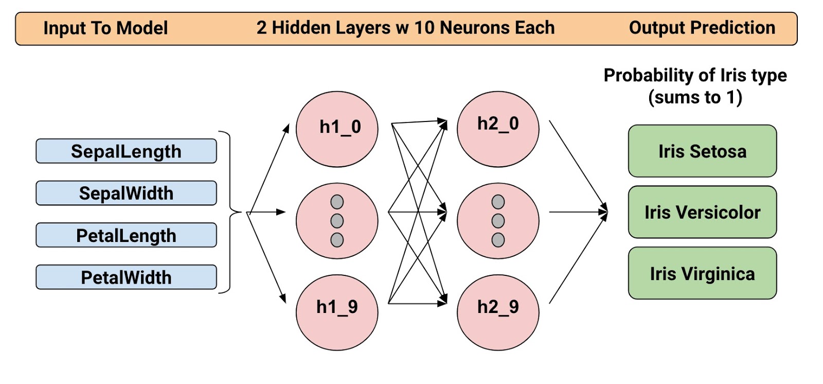
We're going to train a Deep Neural Network Classifier with the below structure. All input and output values will be float32, and the sum of the output values will be 1 (as we are predicting the probability for each individual Iris type):

For example, an output result might be 0.05 for Iris Setosa, 0.9 for Iris Versicolor, and 0.05 for Iris Virginica, which indicates a 90% probability that this is an Iris Versicolor.

Alright! Now that we have defined the model, let's look at how we can use Datasets and Estimators to train it and make predictions.

Introducing The Datasets

Datasets is a new way to create input pipelines to TensorFlow models. This API is much more performant than using feed_dict or the queue-based pipelines, and it's cleaner and easier to use. Although Datasets still resides in tf.contrib.data at 1.3, we expect to move this API to core at 1.4, so it's high time to take it for a test drive.

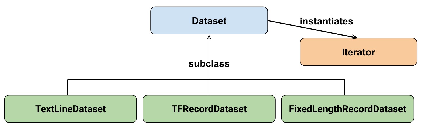
At a high-level, the Datasets consists of the following classes:

Where:

  • Dataset: Base class containing methods to create and transform datasets. Also allows you initialize a dataset from data in memory, or from a Python generator.
  • TextLineDataset: Reads lines from text files.
  • TFRecordDataset: Reads records from TFRecord files.
  • FixedLengthRecordDataset: Reads fixed size records from binary files.
  • Iterator: Provides a way to access one dataset element at a time.

Our dataset

To get started, let's first look at the dataset we will use to feed our model. We'll read data from a CSV file, where each row will contain five values-the four input values, plus the label:

The label will be:

  • 0 for Iris Setosa
  • 1 for Versicolor
  • 2 for Virginica.

Representing our dataset

To describe our dataset, we first create a list of our features:


feature_names = [
'SepalLength',
'SepalWidth',
'PetalLength',
'PetalWidth']

When we train our model, we'll need a function that reads the input file and returns the feature and label data. Estimators requires that you create a function of the following format:


def input_fn():
...<code>...
return ({ 'SepalLength':[values], ..<etc>.., 'PetalWidth':[values] },
[IrisFlowerType])

The return value must be a two-element tuple organized as follows: :

  • The first element must be a dict in which each input feature is a key, and then a list of values for the training batch.
  • The second element is a list of labels for the training batch.

Since we are returning a batch of input features and training labels, it means that all lists in the return statement will have equal lengths. Technically speaking, whenever we referred to "list" here, we actually mean a 1-d TensorFlow tensor.

To allow simple reuse of the input_fn we're going to add some arguments to it. This allows us to build input functions with different settings. The arguments are pretty straightforward:

  • file_path: The data file to read.
  • perform_shuffle: Whether the record order should be randomized.
  • repeat_count: The number of times to iterate over the records in the dataset. For example, if we specify 1, then each record is read once. If we specify None, iteration will continue forever.

Here's how we can implement this function using the Dataset API. We will wrap this in an "input function" that is suitable when feeding our Estimator model later on:

def my_input_fn(file_path, perform_shuffle=False, repeat_count=1):
def decode_csv(line):
parsed_line = tf.decode_csv(line, [[0.], [0.], [0.], [0.], [0]])
label = parsed_line[-1:] # Last element is the label
del parsed_line[-1] # Delete last element
features = parsed_line # Everything (but last element) are the features
d = dict(zip(feature_names, features)), label
return d

dataset = (tf.contrib.data.TextLineDataset(file_path) # Read text file
.skip(1) # Skip header row
.map(decode_csv)) # Transform each elem by applying decode_csv fn
if perform_shuffle:
# Randomizes input using a window of 256 elements (read into memory)
dataset = dataset.shuffle(buffer_size=256)
dataset = dataset.repeat(repeat_count) # Repeats dataset this # times
dataset = dataset.batch(32) # Batch size to use
iterator = dataset.make_one_shot_iterator()
batch_features, batch_labels = iterator.get_next()
return batch_features, batch_labels

Note the following: :

  • TextLineDataset: The Dataset API will do a lot of memory management for you when you're using its file-based datasets. You can, for example, read in dataset files much larger than memory or read in multiple files by specifying a list as argument.
  • shuffle: Reads buffer_size records, then shuffles (randomizes) their order.
  • map: Calls the decode_csv function with each element in the dataset as an argument (since we are using TextLineDataset, each element will be a line of CSV text). Then we apply decode_csv to each of the lines.
  • decode_csv: Splits each line into fields, providing the default values if necessary. Then returns a dict with the field keys and field values. The map function updates each elem (line) in the dataset with the dict.

That's an introduction to Datasets! Just for fun, we can now use this function to print the first batch:

next_batch = my_input_fn(FILE, True) # Will return 32 random elements

# Now let's try it out, retrieving and printing one batch of data.
# Although this code looks strange, you don't need to understand
# the details.
with tf.Session() as sess:
first_batch = sess.run(next_batch)
print(first_batch)

# Output
({'SepalLength': array([ 5.4000001, ...<repeat to 32 elems>], dtype=float32),
'PetalWidth': array([ 0.40000001, ...<repeat to 32 elems>], dtype=float32),
...
},
[array([[2], ...<repeat to 32 elems>], dtype=int32) # Labels
)

That's actually all we need from the Dataset API to implement our model. Datasets have a lot more capabilities though; please see the end of this post where we have collected more resources.

Introducing Estimators

Estimators is a high-level API that reduces much of the boilerplate code you previously needed to write when training a TensorFlow model. Estimators are also very flexible, allowing you to override the default behavior if you have specific requirements for your model.

There are two possible ways you can build your model using Estimators:

  • Pre-made Estimator - These are predefined estimators, created to generate a specific type of model. In this blog post, we will use the DNNClassifier pre-made estimator.
  • Estimator (base class) - Gives you complete control of how your model should be created by using a model_fn function. We will cover how to do this in a separate blog post.

Here is the class diagram for Estimators:

We hope to add more pre-made Estimators in future releases.

As you can see, all estimators make use of input_fn that provides the estimator with input data. In our case, we will reuse my_input_fn, which we defined for this purpose.

The following code instantiates the estimator that predicts the Iris flower type:

# Create the feature_columns, which specifies the input to our model.
# All our input features are numeric, so use numeric_column for each one.
feature_columns = [tf.feature_column.numeric_column(k) for k in feature_names]

# Create a deep neural network regression classifier.
# Use the DNNClassifier pre-made estimator
classifier = tf.estimator.DNNClassifier(
feature_columns=feature_columns, # The input features to our model
hidden_units=[10, 10], # Two layers, each with 10 neurons
n_classes=3,
model_dir=PATH) # Path to where checkpoints etc are stored

We now have a estimator that we can start to train.

Training the model

Training is performed using a single line of TensorFlow code:

# Train our model, use the previously function my_input_fn
# Input to training is a file with training example
# Stop training after 8 iterations of train data (epochs)
classifier.train(
input_fn=lambda: my_input_fn(FILE_TRAIN, True, 8))

But wait a minute... what is this "lambda: my_input_fn(FILE_TRAIN, True, 8)" stuff? That is where we hook up Datasets with the Estimators! Estimators needs data to perform training, evaluation, and prediction, and it uses the input_fn to fetch the data. Estimators require an input_fn with no arguments, so we create a function with no arguments using lambda, which calls our input_fn with the desired arguments: the file_path, shuffle setting, and repeat_count. In our case, we use our my_input_fn, passing it:

  • FILE_TRAIN, which is the training data file.
  • True, which tells the Estimator to shuffle the data.
  • 8, which tells the Estimator to and repeat the dataset 8 times.

Evaluating Our Trained Model

Ok, so now we have a trained model. How can we evaluate how well it's performing? Fortunately, every Estimator contains an evaluatemethod:

# Evaluate our model using the examples contained in FILE_TEST
# Return value will contain evaluation_metrics such as: loss & average_loss
evaluate_result = estimator.evaluate(
input_fn=lambda: my_input_fn(FILE_TEST, False, 4)
print("Evaluation results")
for key in evaluate_result:
print(" {}, was: {}".format(key, evaluate_result[key]))

In our case, we reach an accuracy of about ~93%. There are various ways of improving this accuracy, of course. One way is to simply run the program over and over. Since the state of the model is persisted (in model_dir=PATH above), the model will improve the more iterations you train it, until it settles. Another way would be to adjust the number of hidden layers or the number of nodes in each hidden layer. Feel free to experiment with this; please note, however, that when you make a change, you need to remove the directory specified in model_dir=PATH, since you are changing the structure of the DNNClassifier.

Making Predictions Using Our Trained Model

And that's it! We now have a trained model, and if we are happy with the evaluation results, we can use it to predict an Iris flower based on some input. As with training, and evaluation, we make predictions using a single function call:

# Predict the type of some Iris flowers.
# Let's predict the examples in FILE_TEST, repeat only once.
predict_results = classifier.predict(
input_fn=lambda: my_input_fn(FILE_TEST, False, 1))
print("Predictions on test file")
for prediction in predict_results:
# Will print the predicted class, i.e: 0, 1, or 2 if the prediction
# is Iris Sentosa, Vericolor, Virginica, respectively.
print prediction["class_ids"][0]

Making Predictions on Data in Memory

The preceding code specified FILE_TEST to make predictions on data stored in a file, but how could we make predictions on data residing in other sources, for example, in memory? As you may guess, this does not actually require a change to our predict call. Instead, we configure the Dataset API to use a memory structure as follows:

# Let create a memory dataset for prediction.
# We've taken the first 3 examples in FILE_TEST.
prediction_input = [[5.9, 3.0, 4.2, 1.5], # -> 1, Iris Versicolor
[6.9, 3.1, 5.4, 2.1], # -> 2, Iris Virginica
[5.1, 3.3, 1.7, 0.5]] # -> 0, Iris Sentosa
def new_input_fn():
def decode(x):
x = tf.split(x, 4) # Need to split into our 4 features
# When predicting, we don't need (or have) any labels
return dict(zip(feature_names, x)) # Then build a dict from them

# The from_tensor_slices function will use a memory structure as input
dataset = tf.contrib.data.Dataset.from_tensor_slices(prediction_input)
dataset = dataset.map(decode)
iterator = dataset.make_one_shot_iterator()
next_feature_batch = iterator.get_next()
return next_feature_batch, None # In prediction, we have no labels

# Predict all our prediction_input
predict_results = classifier.predict(input_fn=new_input_fn)

# Print results
print("Predictions on memory data")
for idx, prediction in enumerate(predict_results):
type = prediction["class_ids"][0] # Get the predicted class (index)
if type == 0:
print("I think: {}, is Iris Sentosa".format(prediction_input[idx]))
elif type == 1:
print("I think: {}, is Iris Versicolor".format(prediction_input[idx]))
else:
print("I think: {}, is Iris Virginica".format(prediction_input[idx])

Dataset.from_tensor_slides() is designed for small datasets that fit in memory. When using TextLineDataset as we did for training and evaluation, you can have arbitrarily large files, as long as your memory can manage the shuffle buffer and batch sizes.

Freebies

Using a pre-made Estimator like DNNClassifier provides a lot of value. In addition to being easy to use, pre-made Estimators also provide built-in evaluation metrics, and create summaries you can see in TensorBoard. To see this reporting, start TensorBoard from your command-line as follows:

# Replace PATH with the actual path passed as model_dir argument when the
# DNNRegressor estimator was created.
tensorboard --logdir=PATH

The following diagrams show some of the data that TensorBoard will provide:

Summary

In this this blogpost, we explored Datasets and Estimators. These are important APIs for defining input data streams and creating models, so investing time to learn them is definitely worthwhile!

For more details, be sure to check out

But it doesn't stop here. We will shortly publish more posts that describe how these APIs work, so stay tuned for that!

Until then, Happy TensorFlow coding!

Build your own Machine Learning Visualizations with the new TensorBoard API


When we open-sourced TensorFlow in 2015, it included TensorBoard, a suite of visualizations for inspecting and understanding your TensorFlow models and runs. Tensorboard included a small, predetermined set of visualizations that are generic and applicable to nearly all deep learning applications such as observing how loss changes over time or exploring clusters in high-dimensional spaces. However, in the absence of reusable APIs, adding new visualizations to TensorBoard was prohibitively difficult for anyone outside of the TensorFlow team, leaving out a long tail of potentially creative, beautiful and useful visualizations that could be built by the research community.

To allow the creation of new and useful visualizations, we announce the release of a consistent set of APIs that allows developers to add custom visualization plugins to TensorBoard. We hope that developers use this API to extend TensorBoard and ensure that it covers a wider variety of use cases.

We have updated the existing dashboards (tabs) in TensorBoard to use the new API, so they serve as examples for plugin creators. For the current listing of plugins included within TensorBoard, you can explore the tensorboard/plugins directory on GitHub. For instance, observe the new plugin that generates precision-recall curves:
The plugin demonstrates the 3 parts of a standard TensorBoard plugin:
  • A TensorFlow summary op used to collect data for later visualization. [GitHub]
  • A Python backend that serves custom data. [GitHub]
  • A dashboard within TensorBoard built with TypeScript and polymer. [GitHub]
Additionally, like other plugins, the “pr_curves” plugin provides a demo that (1) users can look over in order to learn how to use the plugin and (2) the plugin author can use to generate example data during development. To further clarify how plugins work, we’ve also created a barebones TensorBoard “Greeter” plugin. This simple plugin collects greetings (simple strings preceded by “Hello, ”) during model runs and displays them. We recommend starting by exploring (or forking) the Greeter plugin as well as other existing plugins.

A notable example of how contributors are already using the TensorBoard API is Beholder, which was recently created by Chris Anderson while working on his master’s degree. Beholder shows a live video feed of data (e.g. gradients and convolution filters) as a model trains. You can watch the demo video here.
We look forward to seeing what innovations will come out of the community. If you plan to contribute a plugin to TensorBoard’s repository, you should get in touch with us first through the issue tracker with your idea so that we can help out and possibly guide you.

Acknowledgements
Dandelion Mané and William Chargin played crucial roles in building this API.