This is a guest post from apertus° and TimVideos.us, open source organizations that participated in Google Summer of Code last year and are back for 2018!
The apertus° AXIOM project is bringing the world’s first open hardware/free software digital motion picture production camera to life. The project has a
rich history, exercises a steadfast adherence to the open source ethos, and all aspects of development have always revolved around supporting and utilising free technologies. The challenge of building a sophisticated digital cinema camera was perfect for
Google Summer of Code 2017. But let’s start at the beginning: why did the team behind the project embark on their journey?
Modern Cinematography
For over a century film was dominated by analog cameras and celluloid, but in the late 2000’s things changed radically with the adoption of digital projection in cinemas. It was a natural next step, then, for filmmakers to shoot and produce films digitally. Certain applications in science, large format photography and fine arts still hold onto 35mm film processing, but the reduction in costs and improved workflows associated with digital image capture have revolutionised how we create and consume visual content.
The DSLR revolution
Filmmaking has long been considered an expensive discipline accessible only to a select few. This all changed with the adoption of movie recording capabilities in
digital single-lens reflex (DSLR) cameras. For multinational corporations this “new” feature was a relatively straightforward addition to existing models as most compact digital photo cameras could already record video clips. This was the first time that a large diameter image sensor, a vital component for creating the typical shallow depth of field we consider cinematic, appeared in consumer cameras. In recent times, user groups have stepped up to contribute to the DSLR revolution first-hand, including groups like the Magic Lantern community.
Magic Lantern
Magic Lantern is a free and open source software add-on that runs from a camera’s SD/CF card. It adds a host of new features to Canon’s DSLRs that weren't included from the factory, such as allowing users to record
high-dynamic range (HDR) video or 14-bit uncompressed
RAW video. It’s a community project and many filmmakers simply wouldn’t have bought a Canon camera if it weren’t for the features that Magic Lantern pioneered. Because installing Magic Lantern doesn’t replace the stock Canon firmware or modify the
read-only memory (ROM) but runs alongside it, it is both easy to remove and carries little risk. Originally developed for filmmaking, Magic Lantern’s feature base has expanded to include tools useful for still photography as well.
Starting the revolution for real
Of course, Magic Lantern has been held back by the underlying proprietary hardware routines on existing camera models. So, in 2014 a team of developers and filmmakers around the
apertus° project joined forces with the Magic Lantern team to lay the foundation for a totally independent, open hardware, free software, digital cinema camera. They ran a
successful crowdfunding campaign for initial development, and they completed hardware development of the first developer kits in 2016. Unlike traditional cameras, the AXIOM is designed to be completely modular, and so continuously evolve, thereby preventing it from ever becoming obsolete. How the camera evolves is determined by its user community, with its design files and source code freely available and users encouraged to duplicate, modify and redistribute anything and everything related to the camera.
While the camera is primarily for use in motion picture production, there are many suitable applications where AXIOM can be useful. Individuals in science, astronomy, medicine, aerial mapping, industrial automation, and those who record events or talks at conferences have expressed interest in the camera. A modular and open source device for digital imaging allows users to build a system that meets their unique requirements. One such company for instance,
Mavrx Inc, who use aerial imagery to provide actionable insight for the agriculture industry, used the camera because it enabled them to not only process the data more efficiently than comparable camera equivalents, but also to re-configure its form factor so that it could be installed alongside existing equipment configurations.
Google Summer of Code 2017
Continuing their journey, apertus° participated in Google Summer of Code for the first time in 2017. They received about 30 applications from interested students, from which they needed to select three. Projects ranged from
field programmable gate array (FPGA) centered video applications to creating
Linux kernel drivers for specific camera hardware. Similarly
TimVideos.us, an open hardware project for live event streaming and conference recording, is working on FPGA projects around video interfaces and processing.
After some preliminary work, the students came to grips with the camera’s operating processes and all three dove in enthusiastically. One student failed the first evaluation and another failed the second, but one student successfully completed their work.
That student,
Vlad Niculescu, worked on defining control loops for a voltage controller using
VHSIC Hardware Description Language (VHDL) for a potential future
AXIOM Beta Power Board, an FPGA-driven smart switching regulator for increasing the power efficiency and improving flexibility around voltage regulation.
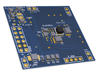  |
| Left: The printed circuit board (PCB) (printed circuit board) for testing the switching regulator FPGA logic. Right: After final improvements the fluctuation ripple in the voltages was reduced to around 30mV at 2V target voltage. |
Vlad had this to say about his experience:
“The knowledge I acquired during my work with this project and apertus° was very satisfying. Besides the electrical skills gained I also managed to obtain other, important universal skills. One of the things I learned was that the key to solving complex problems can often be found by dividing them into small blocks so that the greater whole can be easily observed by others. Writing better code and managing the stages of building a complex project have become lessons that will no doubt become valuable in the future. I will always be grateful to my mentor as he had the patience to explain everything carefully and teach me new things step by step, and also to apertus° and Google’s Summer of Code program, without which I may not have gained the experience of working on a project like this one.”We are grateful for Vlad’s work and congratulate him for successfully completing the program. If you find open hardware and video production interesting, we encourage you to reach out and join the community–both
apertus° and
TimVideos.us are back for Google Summer of Code 2018.
By Sebastian Pichelhofer, apertus°, and Tim 'mithro' Ansell, TimVideos.us