The success of a neural network (NN) often depends on how well it can generalize to various tasks. However, designing NNs that can generalize well is challenging because the research community's understanding of how a neural network generalizes is currently somewhat limited: What does the appropriate neural network look like for a given problem? How deep should it be? Which types of layers should be used? Would LSTMs be enough or would Transformer layers be better? Or maybe a combination of the two? Would ensembling or distillation boost performance? These tricky questions are made even more challenging when considering machine learning (ML) domains where there may exist better intuition and deeper understanding than others.
In recent years, AutoML algorithms have emerged [e.g., 1, 2, 3] to help researchers find the right neural network automatically without the need for manual experimentation. Techniques like neural architecture search (NAS), use algorithms, like reinforcement learning (RL), evolutionary algorithms, and combinatorial search, to build a neural network out of a given search space. With the proper setup, these techniques have demonstrated they are capable of delivering results that are better than the manually designed counterparts. But more often than not, these algorithms are compute heavy, and need thousands of models to train before converging. Moreover, they explore search spaces that are domain specific and incorporate substantial prior human knowledge that does not transfer well across domains. As an example, in image classification, the traditional NAS searches for two good building blocks (convolutional and downsampling blocks), that it arranges following traditional conventions to create the full network.
To overcome these shortcomings and to extend access to AutoML solutions to the broader research community, we are excited to announce the open source release of Model Search, a platform that helps researchers develop the best ML models, efficiently and automatically. Instead of focusing on a specific domain, Model Search is domain agnostic, flexible and is capable of finding the appropriate architecture that best fits a given dataset and problem, while minimizing coding time, effort and compute resources. It is built on Tensorflow, and can run either on a single machine or in a distributed setting.
Overview
The Model Search system consists of multiple trainers, a search algorithm, a transfer learning algorithm and a database to store the various evaluated models. The system runs both training and evaluation experiments for various ML models (different architectures and training techniques) in an adaptive, yet asynchronous, fashion. While each trainer conducts experiments independently, all trainers share the knowledge gained from their experiments. At the beginning of every cycle, the search algorithm looks up all the completed trials and uses beam search to decide what to try next. It then invokes mutation over one of the best architectures found thus far and assigns the resulting model back to a trainer.
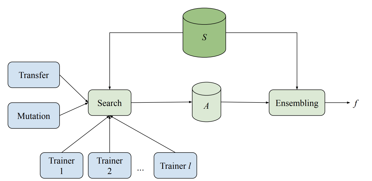 |
| Model Search schematic illustrating the distributed search and ensembling. Each trainer runs independently to train and evaluate a given model. The results are shared with the search algorithm, which it stores. The search algorithm then invokes mutation over one of the best architectures and then sends the new model back to a trainer for the next iteration. S is the set of training and validation examples and A are all the candidates used during training and search. |
The system builds a neural network model from a set of predefined blocks, each of which represents a known micro-architecture, like LSTM, ResNet or Transformer layers. By using blocks of pre-existing architectural components, Model Search is able to leverage existing best knowledge from NAS research across domains. This approach is also more efficient, because it explores structures, not their more fundamental and detailed components, therefore reducing the scale of the search space.
 |
| Neural network micro architecture blocks that work well, e.g., a ResNet Block. |
Because the Model Search framework is built on Tensorflow, blocks can implement any function that takes a tensor as an input. For example, imagine that one wants to introduce a new search space built with a selection of micro architectures. The framework will take the newly defined blocks and incorporate them into the search process so that algorithms can build the best possible neural network from the components provided. The blocks provided can even be fully defined neural networks that are already known to work for the problem of interest. In that case, Model Search can be configured to simply act as a powerful ensembling machine.
The search algorithms implemented in Model Search are adaptive, greedy and incremental, which makes them converge faster than RL algorithms. They do however imitate the “explore & exploit” nature of RL algorithms by separating the search for a good candidate (explore step), and boosting accuracy by ensembling good candidates that were discovered (exploit step). The main search algorithm adaptively modifies one of the top k performing experiments (where k can be specified by the user) after applying random changes to the architecture or the training technique (e.g., making the architecture deeper).
 |
| An example of an evolution of a network over many experiments. Each color represents a different type of architecture block. The final network is formed via mutations of high performing candidate networks, in this case adding depth. |
To further improve efficiency and accuracy, transfer learning is enabled between various internal experiments. Model Search does this in two ways — via knowledge distillation or weight sharing. Knowledge distillation allows one to improve candidates' accuracies by adding a loss term that matches the high performing models’ predictions in addition to the ground truth. Weight sharing, on the other hand, bootstraps some of the parameters (after applying mutation) in the network from previously trained candidates by copying suitable weights from previously trained models and randomly initializing the remaining ones. This enables faster training, which allows opportunities to discover more (and better) architectures.
Experimental Results
Model Search improves upon production models with minimal iterations. In a recent paper, we demonstrated the capabilities of Model Search in the speech domain by discovering a model for keyword spotting and language identification. Over fewer than 200 iterations, the resulting model slightly improved upon internal state-of-the-art production models designed by experts in accuracy using ~130K fewer trainable parameters (184K compared to 315K parameters).
 |
| Model accuracy given iteration in our system compared to the previous production model for keyword spotting, a similar graph can be found for language identification in the linked paper. |
We also applied Model Search to find an architecture suitable for image classification on the heavily explored CIFAR-10 imaging dataset. Using a set known convolution blocks, including convolutions, resnet blocks (i.e., two convolutions and a skip connection), NAS-A cells, fully connected layers, etc., we observed that we were able to quickly reach a benchmark accuracy of 91.83 in 209 trials (i.e., exploring only 209 models). In comparison, previous top performers reached the same threshold accuracy in 5807 trials for the NasNet algorithm (RL), and 1160 for PNAS (RL + Progressive).
Conclusion
We hope the Model Search code will provide researchers with a flexible, domain-agnostic framework for ML model discovery. By building upon previous knowledge for a given domain, we believe that this framework is powerful enough to build models with the state-of-the-art performance on well studied problems when provided with a search space composed of standard building blocks.
Acknowledgements
Special thanks to all code contributors to the open sourcing and the paper: Eugen Ehotaj, Scotty Yak, Malaika Handa, James Preiss, Pai Zhu, Aleks Kracun, Prashant Sridhar, Niranjan Subrahmanya, Ignacio Lopez Moreno, Hyun Jin Park, and Patrick Violette.


