Tag Archives: Visualization

The What-If Tool: Code-Free Probing of Machine Learning Models


Building effective machine learning (ML) systems means asking a lot of questions. It's not enough to train a model and walk away. Instead, good practitioners act as detectives, probing to understand their model better: How would changes to a datapoint affect my model’s prediction? Does it perform differently for various groups–for example, historically marginalized people? How diverse is the dataset I am testing my model on?

Answering these kinds of questions isn’t easy. Probing “what if” scenarios often means writing custom, one-off code to analyze a specific model. Not only is this process inefficient, it makes it hard for non-programmers to participate in the process of shaping and improving ML models. One focus of the Google AI PAIR initiative is making it easier for a broad set of people to examine, evaluate, and debug ML systems.

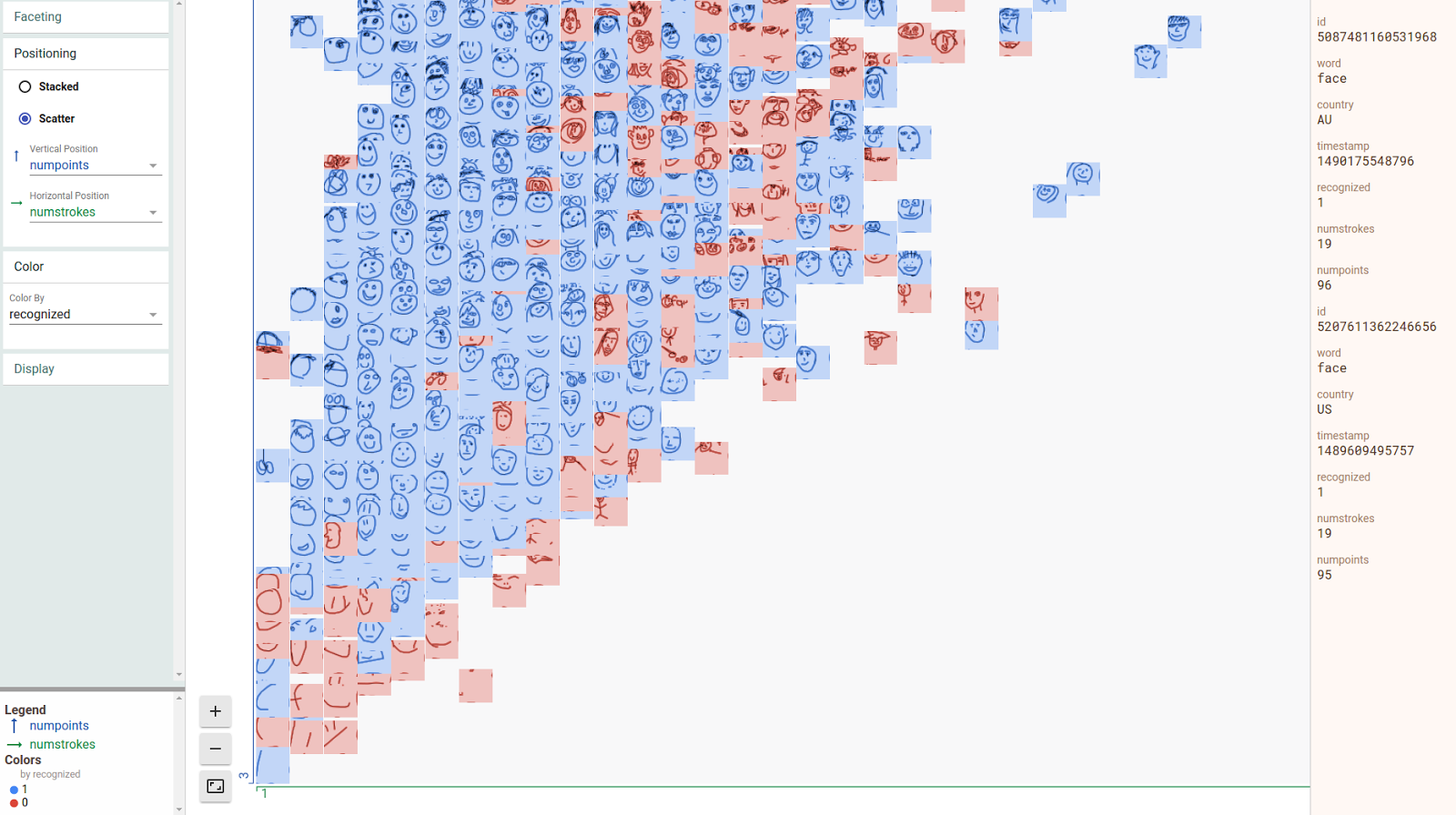
Today, we are launching the What-If Tool, a new feature of the open-source TensorBoard web application, which let users analyze an ML model without writing code. Given pointers to a TensorFlow model and a dataset, the What-If Tool offers an interactive visual interface for exploring model results.
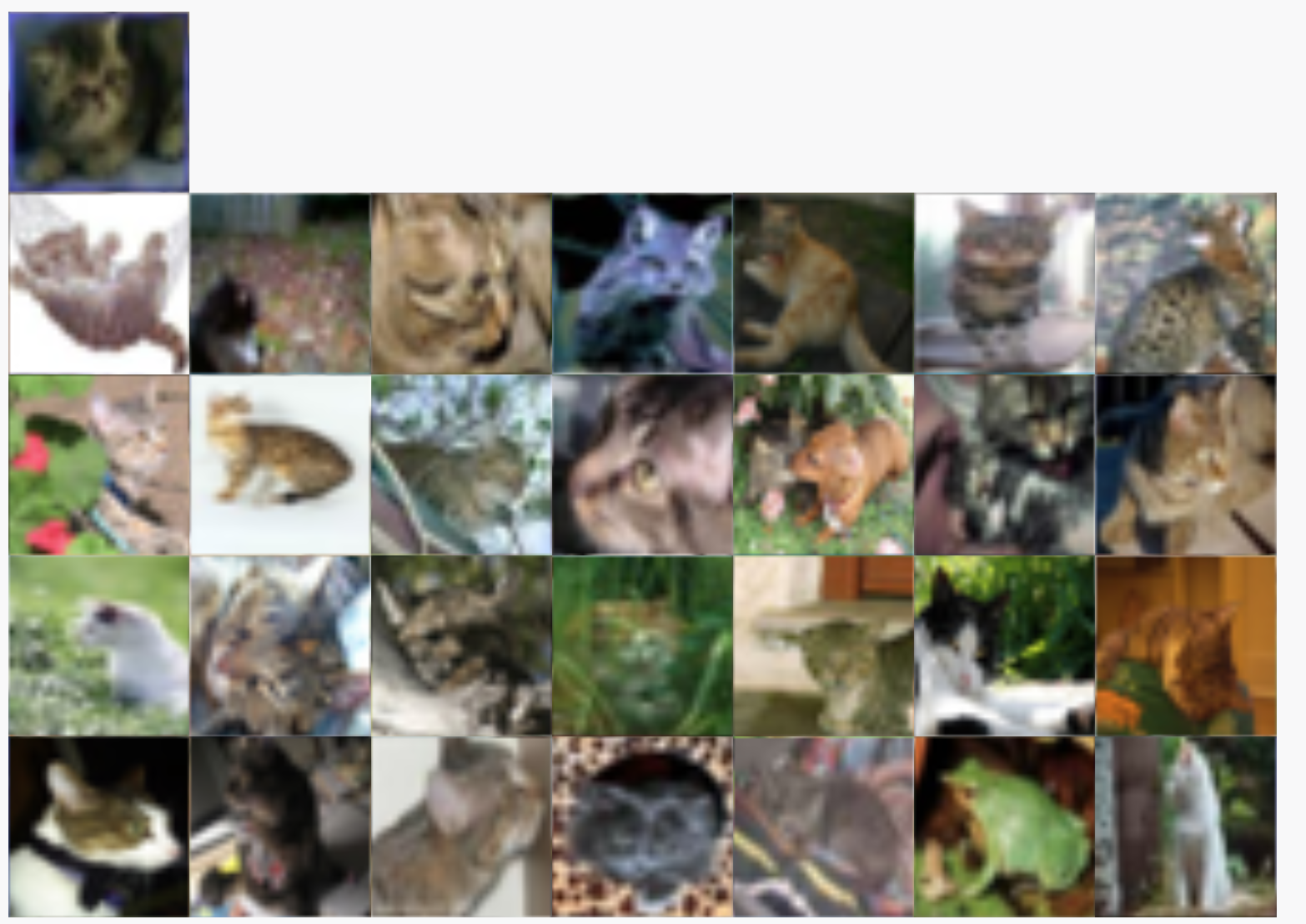
The What-If Tool, showing a set of 250 face pictures and their results from a model that detects smiles.
The What-If Tool has a large set of features, including visualizing your dataset automatically using Facets, the ability to manually edit examples from your dataset and see the effect of those changes, and automatic generation of partial dependence plots which show how the model’s predictions change as any single feature is changed. Let’s explore two features in more detail.
Exploring what-if scenarios on a datapoint.
Counterfactuals
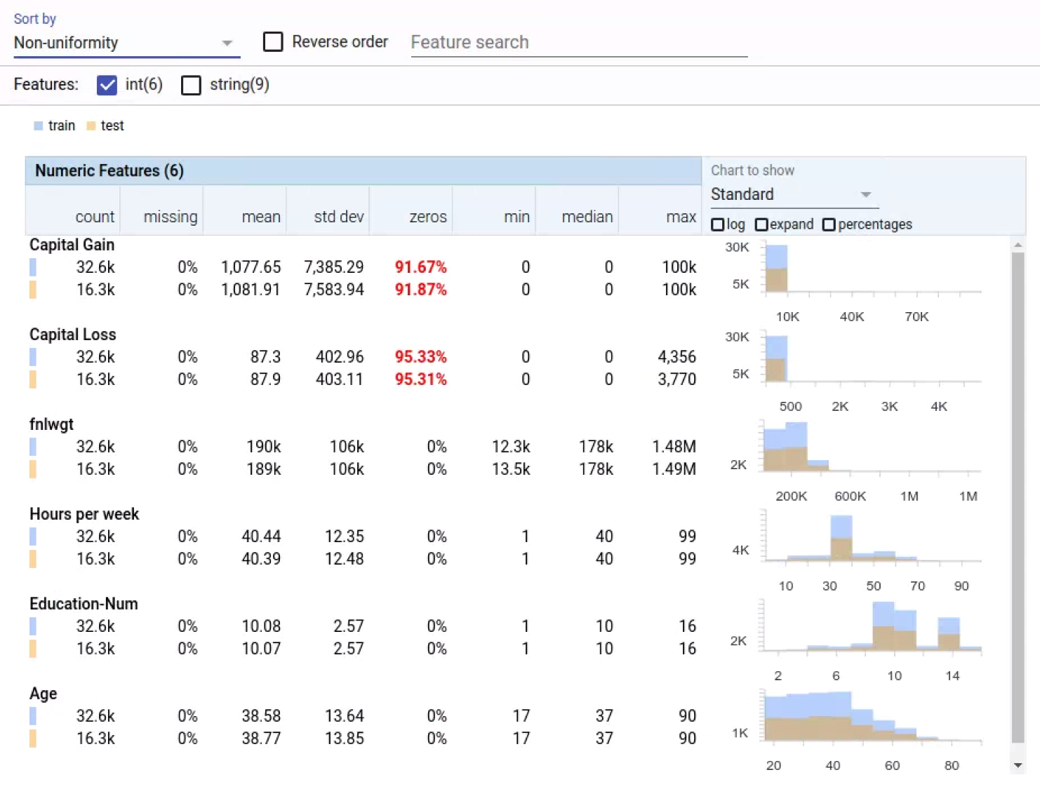
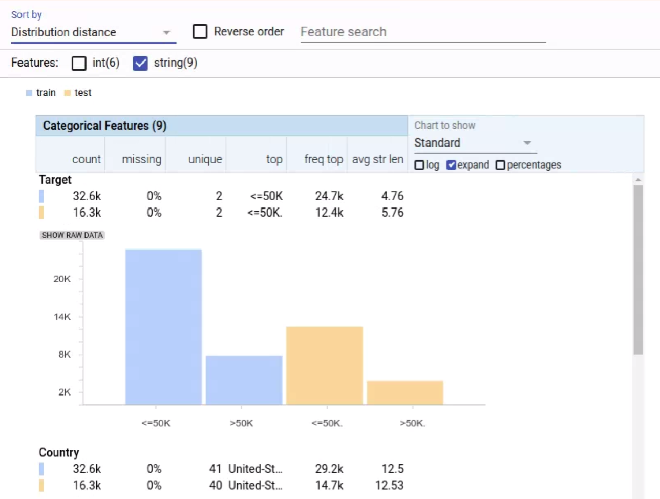
With a click of a button you can compare a datapoint to the most similar point where your model predicts a different result. We call such points "counterfactuals," and they can shed light on the decision boundaries of your model. Or, you can edit a datapoint by hand and explore how the model’s prediction changes. In the screenshot below, the tool is being used on a binary classification model that predicts whether a person earns more than $50k based on public census data from the UCI census dataset. This is a benchmark prediction task used by ML researchers, especially when analyzing algorithmic fairness — a topic we'll get to soon. In this case, for the selected datapoint, the model predicted with 73% confidence that the person earns more than $50k. The tool has automatically located the most-similar person in the dataset for which the model predicted earnings of less than $50k and compares the two side-by-side. In this case, with just a minor difference in age and an occupation change, the model’s prediction has flipped.
Comparing counterfactuals.
Analysis of Performance and Algorithmic Fairness
You can also explore the effects of different classification thresholds, taking into account constraints such as different numerical fairness criteria. The below screenshot shows the results of a smile detector model, trained on the open-source CelebA dataset which consists of annotated face images of celebrities. Below, the faces in the dataset are divided by whether they have brown hair, and for each of the two groups there is an ROC curve and confusion matrix of the predictions, along with sliders for setting how confident the model must be before determining that a face is smiling. In this case, the confidence thresholds for the two groups were set automatically by the tool to optimize for equal opportunity.
Comparing the performance of two slices of data on a smile detection model, with their classification thresholds set to satisfy the “equal opportunity” constraint.
Demos
To illustrate the capabilities of the What-If Tool, we’ve released a set of demos using pre-trained models:
  • Detecting misclassifications: A multiclass classification model, which predicts plant type from four measurements of a flower from the plant. The tool is helpful in showing the decision boundary of the model and what causes misclassifications. This model is trained with the UCI iris dataset.
  • Assessing fairness in binary classification models: The image classification model for smile detection mentioned above. The tool is helpful in assessing algorithmic fairness across different subgroups. The model was purposefully trained without providing any examples from a specific subset of the population, in order to show how the tool can help uncover such biases in models. Assessing fairness requires careful consideration of the overall context — but this is a useful quantitative starting point.
  • Investigating model performance across different subgroups: A regression model that predicts a subject’s age from census information. The tool is helpful in showing relative performance of the model across subgroups and how the different features individually affect the prediction. This model is trained with the UCI census dataset.
What-If in Practice
We tested the What-If Tool with teams inside Google and saw the immediate value of such a tool. One team quickly found that their model was incorrectly ignoring an entire feature of their dataset, leading them to fix a previously-undiscovered code bug. Another team used it to visually organize their examples from best to worst performance, leading them to discover patterns about the types of examples their model was underperforming on.

We look forward to people inside and outside of Google using this tool to better understand ML models and to begin assessing fairness. And as the code is open-source, we welcome contributions to the tool.

Acknowledgments
The What-If Tool was a collaborative effort, with UX design by Mahima Pushkarna, Facets updates by Jimbo Wilson, and input from many others. We would like to thank the Google teams that piloted the tool and provided valuable feedback and the TensorBoard team for all their help.

Source: Google AI Blog


Realtime tSNE Visualizations with TensorFlow.js


In recent years, the t-distributed Stochastic Neighbor Embedding (tSNE) algorithm has become one of the most used and insightful techniques for exploratory data analysis of high-dimensional data. Used to interpret deep neural network outputs in tools such as the TensorFlow Embedding Projector and TensorBoard, a powerful feature of tSNE is that it reveals clusters of high-dimensional data points at different scales while requiring only minimal tuning of its parameters. Despite these advantages, the computational complexity of the tSNE algorithm limits its application to relatively small datasets. While several evolutions of tSNE have been developed to address this issue (mainly focusing on the scalability of the similarity computations between data points), they have so far not been enough to provide a truly interactive experience when visualizing the evolution of the tSNE embedding for large datasets.

In “Linear tSNE Optimization for the Web”, we present a novel approach to tSNE that heavily relies on modern graphics hardware. Given the linear complexity of the new approach, our method generates embeddings faster than comparable techniques and can even be executed on the client side in a web browser by leveraging GPU capabilities through WebGL. The combination of these two factors allows for real-time interactive visualization of large, high-dimensional datasets. Furthermore, we are releasing this work as an open source library in the TensorFlow.js family in the hopes that the broader research community finds it useful.
Real-time evolution of the tSNE embedding for the complete MNIST dataset with our technique. The dataset contains images of 60,000 handwritten digits. You can find a live demo here.
The aim of tSNE is to cluster small “neighborhoods” of similar data points while also reducing the overall dimensionality of the data so it is more easily visualized. In other words, the tSNE objective function measures how well these neighborhoods of similar data are preserved in the 2 or 3-dimensional space, and arranges them into clusters accordingly.

In previous work, the minimization of the tSNE objective was performed as a N-body simulation problem, in which points are randomly placed in the embedding space and two different types of forces are applied on each point. Attractive forces bring the points closer to the points that are most similar in the high-dimensional space, while repulsive forces push them away from all the neighbors in the embedding.

While the attractive forces are acting on a small subset of points (i.e., similar neighbors), repulsive forces are in effect from all pairs of points. Due to this, tSNE requires significant computation and many iterations of the objective function, which limits the possible dataset size to just a few hundred data points. To improve over a brute force solution, the Barnes-Hut algorithm was used to approximate the repulsive forces and the gradient of the objective function. This allows scaling of the computation to tens of thousand data points, but it requires more than 15 minutes to compute the MNIST embedding in a C++ implementation.

In our paper, we propose a solution to this scaling problem by approximating the gradient of the objective function using textures that are generated in WebGL. Our technique draws a “repulsive field” at every minimization iteration using a three channel texture, with the 3 components treated as colors and drawn in the RGB channels. The repulsive field is obtained for every point to represent both the horizontal and vertical repulsive force created by the point, and a third component used for normalization. Intuitively, the normalization term ensures that the magnitude of the shifts matches the similarity measure in the high-dimensional space. In addition, the resolution of the texture is adaptively changed to keep the number of pixels drawn constant.
Rendering of the three functions used to approximate the repulsive effect created by a single point. In the above figure the repulsive forces show a point in a blue area is pushed to the left/bottom, while a point in the red area is pushed to the right/top while a point in the white region will not move.
The contribution of every point is then added on the GPU, resulting in a texture similar to those presented in the GIF below, that approximate the repulsive fields. This innovative repulsive field approach turns out to be much more GPU friendly than more commonly used calculation of point-to-point interactions. This is because repulsion for multiple points can be computed at once and in a very fast way in the GPU. In addition, we implemented the computation of the attraction between points in the GPU.
This animation shows the evolution of the tSNE embedding (upper left) and of the scalar fields used to approximate its gradient with normalization term (upper right), horizontal shift (bottom left) and vertical shift (bottom right).
We additionally revised the update of the embedding from an ad-hoc implementation to a series of standard tensor operations that are computed in TensorFlow.js, a JavaScript library to perform tensor computations in the web browser. Our approach, which is released as an open source library in the TensorFlow.js family, allows us to compute the evolution of the tSNE embedding entirely on the GPU while having better computational complexity.

With this implementation, what used to take 15 minutes to calculate (on the MNIST dataset) can now be visualized in real-time and in the web browser. Furthermore this allows real-time visualizations of much larger datasets, a feature that is particularly useful when deep neural output is analyzed. One main limitation of our work is that this technique currently only works for 2D embeddings. However, 2D visualizations are often preferred over 3D ones as they require more interaction to effectively understand cluster results.

Future Work
We believe that having a fast and interactive tSNE implementation that runs in the browser will empower developers of data analytics systems. We are particularly interested in exploring how our implementation can be used for the interpretation of deep neural networks. Additionally, our implementation shows how lateral thinking in using GPU computations (approximating the gradient using RGB texture) can be used to significantly speed up algorithmic computations. In the future we will be exploring how this kind of gradient approximation can be applied not only to speed-up other dimensionality reduction algorithms, but also to implement other N-body simulations in the web browser using TensorFlow.js.

Acknowledgements
We would like to thank Alexander Mordvintsev, Yannick Assogba, Matt Sharifi, Anna Vilanova, Elmar Eisemann, Nikhil Thorat, Daniel Smilkov, Martin Wattenberg, Fernanda Viegas, Alessio Bazzica, Boudewijn Lelieveldt, Thomas Höllt, Baldur van Lew, Julian Thijssen and Marvin Ritter.

Source: Google AI Blog


The Building Blocks of Interpretability


(Crossposted on the Google Open Source Blog)

In 2015, our early attempts to visualize how neural networks understand images led to psychedelic images. Soon after, we open sourced our code as DeepDream and it grew into a small art movement producing all sorts of amazing things. But we also continued the original line of research behind DeepDream, trying to address one of the most exciting questions in Deep Learning: how do neural networks do what they do?

Last year in the online journal Distill, we demonstrated how those same techniques could show what individual neurons in a network do, rather than just what is “interesting to the network” as in DeepDream. This allowed us to see how neurons in the middle of the network are detectors for all sorts of things — buttons, patches of cloth, buildings — and see how those build up to be more and more sophisticated over the networks layers.
Visualizations of neurons in GoogLeNet. Neurons in higher layers represent higher level ideas.
While visualizing neurons is exciting, our work last year was missing something important: how do these neurons actually connect to what the network does in practice?

Today, we’re excited to publish “The Building Blocks of Interpretability,” a new Distill article exploring how feature visualization can combine together with other interpretability techniques to understand aspects of how networks make decisions. We show that these combinations can allow us to sort of “stand in the middle of a neural network” and see some of the decisions being made at that point, and how they influence the final output. For example, we can see things like how a network detects a floppy ear, and then that increases the probability it gives to the image being a “Labrador retriever” or “beagle”.

We explore techniques for understanding which neurons fire in the network. Normally, if we ask which neurons fire, we get something meaningless like “neuron 538 fired a little bit,” which isn’t very helpful even to experts. Our techniques make things more meaningful to humans by attaching visualizations to each neuron, so we can see things like “the floppy ear detector fired”. It’s almost a kind of MRI for neural networks.
We can also zoom out and show how the entire image was “perceived” at different layers. This allows us to really see the transition from the network detecting very simple combinations of edges, to rich textures and 3d structure, to high-level structures like ears, snouts, heads and legs.
These insights are exciting by themselves, but they become even more exciting when we can relate them to the final decision the network makes. So not only can we see that the network detected a floppy ear, but we can also see how that increases the probability of the image being a labrador retriever.
In addition to our paper, we’re also releasing Lucid, a neural network visualization library building off our work on DeepDream. It allows you to make the sort lucid feature visualizations we see above, in addition to more artistic DeepDream images.

We’re also releasing colab notebooks. These notebooks make it extremely easy to use Lucid to reproduce visualizations in our article! Just open the notebook, click a button to run code — no setup required!
In colab notebooks you can click a button to run code, and see the result below.
This work only scratches the surface of the kind of interfaces that we think it’s possible to build for understanding neural networks. We’re excited to see what the community will do — and we’re excited to work together towards deeper human understanding of neural networks.

Feature Visualization


Have you ever wondered what goes on inside neural networks? Feature visualization is a powerful tool for digging into neural networks and seeing how they work.

Our new article, published in Distill, does a deep exploration of feature visualization, introducing a few new tricks along the way!

Building on our work in DeepDream, and lots of work by others since, we are able to visualize what every neuron a strong vision model (GoogLeNet [1]) detects. Over the course of multiple layers, it gradually builds up abstractions: first it detects edges, then it uses those edges to detect textures, the textures to detect patterns, and the patterns to detect parts of objects….
But neurons don’t understand the world by themselves — they work together. So we also need to understand how they interact with each other. One approach is to explore interpolations between them. What images can make them both fire, to different extents?

Here we interpolate from a neuron that seems to detect artistic patterns to a neuron that seems to detect lizard eyes:
We can also let you try adding different pairs of neurons together, to explore the possibilities for yourself:
In addition to allowing you to play around with visualizations, we explore a variety of techniques for getting feature visualization to work, and let you experiment with using them.
Techniques for visualizing and understanding neural networks are becoming more powerful. We hope our article will help other researchers apply these techniques, and give people a sense of their potential. Check it out on Distill.

Acknowledgement
We're extremely grateful to our co-author, Ludwig Schurbert, who made incredible contributions to our paper and especially to the interactive visualizations.


Build your own Machine Learning Visualizations with the new TensorBoard API


When we open-sourced TensorFlow in 2015, it included TensorBoard, a suite of visualizations for inspecting and understanding your TensorFlow models and runs. Tensorboard included a small, predetermined set of visualizations that are generic and applicable to nearly all deep learning applications such as observing how loss changes over time or exploring clusters in high-dimensional spaces. However, in the absence of reusable APIs, adding new visualizations to TensorBoard was prohibitively difficult for anyone outside of the TensorFlow team, leaving out a long tail of potentially creative, beautiful and useful visualizations that could be built by the research community.

To allow the creation of new and useful visualizations, we announce the release of a consistent set of APIs that allows developers to add custom visualization plugins to TensorBoard. We hope that developers use this API to extend TensorBoard and ensure that it covers a wider variety of use cases.

We have updated the existing dashboards (tabs) in TensorBoard to use the new API, so they serve as examples for plugin creators. For the current listing of plugins included within TensorBoard, you can explore the tensorboard/plugins directory on GitHub. For instance, observe the new plugin that generates precision-recall curves:
The plugin demonstrates the 3 parts of a standard TensorBoard plugin:
  • A TensorFlow summary op used to collect data for later visualization. [GitHub]
  • A Python backend that serves custom data. [GitHub]
  • A dashboard within TensorBoard built with TypeScript and polymer. [GitHub]
Additionally, like other plugins, the “pr_curves” plugin provides a demo that (1) users can look over in order to learn how to use the plugin and (2) the plugin author can use to generate example data during development. To further clarify how plugins work, we’ve also created a barebones TensorBoard “Greeter” plugin. This simple plugin collects greetings (simple strings preceded by “Hello, ”) during model runs and displays them. We recommend starting by exploring (or forking) the Greeter plugin as well as other existing plugins.

A notable example of how contributors are already using the TensorBoard API is Beholder, which was recently created by Chris Anderson while working on his master’s degree. Beholder shows a live video feed of data (e.g. gradients and convolution filters) as a model trains. You can watch the demo video here.
We look forward to seeing what innovations will come out of the community. If you plan to contribute a plugin to TensorBoard’s repository, you should get in touch with us first through the issue tracker with your idea so that we can help out and possibly guide you.

Acknowledgements
Dandelion Mané and William Chargin played crucial roles in building this API.


Harness the Power of Machine Learning in Your Browser with Deeplearn.js


Machine learning (ML) has become an increasingly powerful tool, one that can be applied to a wide variety of areas spanning object recognition, language translation, health and more. However, the development of ML systems is often restricted to those with computational resources and the technical expertise to work with commonly available ML libraries.

With PAIR — an initiative to study and redesign human interactions with ML — we want to open machine learning up to as many people as possible. In pursuit of that goal, we are excited to announce deeplearn.js 0.1.0, an open source WebGL-accelerated JavaScript library for machine learning that runs entirely in your browser, with no installations and no backend.
There are many reasons to bring machine learning into the browser. A client-side ML library can be a platform for interactive explanations, for rapid prototyping and visualization, and even for offline computation. And if nothing else, the browser is one of the world's most popular programming platforms.

While web machine learning libraries have existed for years (e.g., Andrej Karpathy's convnetjs) they have been limited by the speed of Javascript, or have been restricted to inference rather than training (e.g., TensorFire). By contrast, deeplearn.js offers a significant speedup by exploiting WebGL to perform computations on the GPU, along with the ability to do full backpropagation.

The API mimics the structure of TensorFlow and NumPy, with a delayed execution model for training (like TensorFlow), and an immediate execution model for inference (like NumPy). We have also implemented versions of some of the most commonly-used TensorFlow operations. With the release of deeplearn.js, we will be providing tools to export weights from TensorFlow checkpoints, which will allow authors to import them into web pages for deeplearn.js inference.

You can explore the potential of this library by training a convolutional neural network to recognize photos and handwritten digits — all in your browser without writing a single line of code.
We're releasing a series of demos that show deeplearn.js in action. Play with an image classifier that uses your webcam in real-time and watch the network’s internal representations of what it sees. Or generate abstract art videos at a smooth 60 frames per second. The deeplearn.js homepage contains these and other demos.

Our vision is that this library will significantly increase visibility and engagement with machine learning, giving developers access to powerful tools while simultaneously providing the everyday user with a way to interact with them. We’re looking forward to collaborating with the open source community to drive this vision forward.

Facets: An Open Source Visualization Tool for Machine Learning Training Data


(Cross-posted on the Google Open Source Blog)

Getting the best results out of a machine learning (ML) model requires that you truly understand your data. However, ML datasets can contain hundreds of millions of data points, each consisting of hundreds (or even thousands) of features, making it nearly impossible to understand an entire dataset in an intuitive fashion. Visualization can help unlock nuances and insights in large datasets. A picture may be worth a thousand words, but an interactive visualization can be worth even more.

Working with the PAIR initiative, we’ve released Facets, an open source visualization tool to aid in understanding and analyzing ML datasets. Facets consists of two visualizations that allow users to see a holistic picture of their data at different granularities. Get a sense of the shape of each feature of the data using Facets Overview, or explore a set of individual observations using Facets Dive. These visualizations allow you to debug your data which, in machine learning, is as important as debugging your model. They can easily be used inside of Jupyter notebooks or embedded into webpages. In addition to the open source code, we've also created a Facets demo website. This website allows anyone to visualize their own datasets directly in the browser without the need for any software installation or setup, without the data ever leaving your computer.

Facets Overview
Facets Overview automatically gives users a quick understanding of the distribution of values across the features of their datasets. Multiple datasets, such as a training set and a test set, can be compared on the same visualization. Common data issues that can hamper machine learning are pushed to the forefront, such as: unexpected feature values, features with high percentages of missing values, features with unbalanced distributions, and feature distribution skew between datasets.
Facets Overview visualization of the six numeric features of the UCI Census datasets[1]. The features are sorted by non-uniformity, with the feature with the most non-uniform distribution at the top. Numbers in red indicate possible trouble spots, in this case numeric features with a high percentage of values set to 0. The histograms at right allow you to compare the distributions between the training data (blue) and test data (orange).

Facets Overview visualization showing two of the nine categorical features of the UCI Census datasets[1]. The features are sorted by distribution distance, with the feature with the biggest skew between the training (blue) and test (orange) datasets at the top. Notice in the “Target” feature that the label values differ between the training and test datasets, due to a trailing period in the test set (“<=50K” vs “<=50K.”). This can be seen in the chart for the feature and also in the entries in the “top” column of the table. This label mismatch would cause a model trained and tested on this data to not be evaluated correctly.
Facets Dive
Facets Dive provides an easy-to-customize, intuitive interface for exploring the relationship between the data points across the different features of a dataset. With Facets Dive, you control the position, color and visual representation of each data point based on its feature values. If the data points have images associated with them, the images can be used as the visual representations.
Facets Dive visualization showing all 16281 data points in the UCI Census test dataset[1]. The animation shows a user coloring the data points by one feature (“Relationship”), faceting in one dimension by a continuous feature (“Age”) and then faceting in another dimension by a discrete feature (“Marital Status”).
Facets Dive visualization of a large number of face drawings from the “Quick, Draw!” Dataset, showing the relationship between the number of strokes and points in the drawings and the ability for the “Quick, Draw!” classifier to correctly categorize them as faces.
Fun Fact: In large datasets, such as the CIFAR-10 dataset[2], a small human labelling error can easily go unnoticed. We inspected the CIFAR-10 dataset with Dive and were able to catch a frog-cat – an image of a frog that had been incorrectly labelled as a cat!
Exploration of the CIFAR-10 dataset using Facets Dive. Here we facet the ground truth labels by row and the predicted labels by column. This produces a confusion matrix view, allowing us to drill into particular kinds of misclassifications. In this particular case, the ML model incorrectly labels some small percentage of true cats as frogs. The interesting thing we find by putting the real images in the confusion matrix is that one of these "true cats" that the model predicted was a frog is actually a frog from visual inspection. With Facets Dive, we can determine that this one misclassification wasn't a true misclassification of the model, but instead incorrectly labeled data in the dataset.
Can you spot the frog-cat?

We’ve gotten great value out of Facets inside of Google and are excited to share the visualizations with the world. We hope they can help you discover new and interesting things about your data that lead you to create more powerful and accurate machine learning models. And since they are open source, you can customize the visualizations for your specific needs or contribute to the project to help us all better understand our data. If you have feedback about your experience with Facets, please let us know what you think.

Acknowledgments
This work is a collaboration between Mahima Pushkarna, James Wexler and Jimbo Wilson, with input from the entire Big Picture team. We would also like to thank Justine Tunney for providing us with the build tooling.

References
[1] Lichman, M. (2013). UCI Machine Learning Repository [http://archive.ics.uci.edu/ml/datasets/Census+Income]. Irvine, CA: University of California, School of Information and Computer Science

[2] Learning Multiple Layers of Features from Tiny Images, Alex Krizhevsky, 2009.

Facets: An Open Source Visualization Tool for Machine Learning Training Data

Cross-posted on the Google Research Blog

Getting the best results out of a machine learning (ML) model requires that you truly understand your data. However, ML datasets can contain hundreds of millions of data points, each consisting of hundreds (or even thousands) of features, making it nearly impossible to understand an entire dataset in an intuitive fashion. Visualization can help unlock nuances and insights in large datasets. A picture may be worth a thousand words, but an interactive visualization can be worth even more.

Working with the PAIR initiative, we’ve released Facets, an open source visualization tool to aid in understanding and analyzing ML datasets. Facets consists of two visualizations that allow users to see a holistic picture of their data at different granularities. Get a sense of the shape of each feature of the data using Facets Overview, or explore a set of individual observations using Facets Dive. These visualizations allow you to debug your data which, in machine learning, is as important as debugging your model. They can easily be used inside of Jupyter notebooks or embedded into webpages. In addition to the open source code, we've also created a Facets demo website. This website allows anyone to visualize their own datasets directly in the browser without the need for any software installation or setup, without the data ever leaving your computer.

Facets Overview

Facets Overview automatically gives users a quick understanding of the distribution of values across the features of their datasets. Multiple datasets, such as a training set and a test set, can be compared on the same visualization. Common data issues that can hamper machine learning are pushed to the forefront, such as: unexpected feature values, features with high percentages of missing values, features with unbalanced distributions, and feature distribution skew between datasets.
overview-numerical.png
Facets Overview visualization of the six numeric features of the UCI Census datasets[1]. The features are sorted by non-uniformity, with the feature with the most non-uniform distribution at the top. Numbers in red indicate possible trouble spots, in this case numeric features with a high percentage of values set to 0. The histograms at right allow you to compare the distributions between the training data (blue) and test data (orange).

overview-categorical-expand.png
Facets Overview visualization showing two of the nine categorical features of the UCI Census datasets[1]. The features are sorted by distribution distance, with the feature with the biggest skew between the training (blue) and test (orange) datasets at the top. Notice in the “Target” feature that the label values differ between the training and test datasets, due to a trailing period in the test set (“<=50K” vs “<=50K.”). This can be seen in the chart for the feature and also in the entries in the “top” column of the table. This label mismatch would cause a model trained and tested on this data to not be evaluated correctly.

Facets Dive

Facets Dive provides an easy-to-customize, intuitive interface for exploring the relationship between the data points across the different features of a dataset. With Facets Dive, you control the position, color and visual representation of each data point based on its feature values. If the data points have images associated with them, the images can be used as the visual representations.
facets-dive.gif
Facets Dive visualization showing all 16281 data points in the UCI Census test dataset[1]. The animation shows a user coloring the data points by one feature (“Relationship”), faceting in one dimension by a continuous feature (“Age”) and then faceting in another dimension by a discrete feature (“Marital Status”).
dive-quickdraw.png
Facets Dive visualization of a large number of face drawings from the “Quick, Draw!” Dataset, showing the relationship between the number of strokes and points in the drawings and the ability for the “Quick, Draw!” classifier to correctly categorize them as faces.

Fun Fact: In large datasets, such as the CIFAR-10 dataset[2], a small human labelling error can easily go unnoticed. We inspected the CIFAR-10 dataset with Dive and were able to catch a frog-cat – an image of a frog that had been incorrectly labelled as a cat!
cat-frogs.gif
Exploration of the CIFAR-10 dataset using Facets Dive. Here we facet the ground truth labels by row and the predicted labels by column. This produces a confusion matrix view, allowing us to drill into particular kinds of misclassifications. In this particular case, the ML model incorrectly labels some small percentage of true cats as frogs. The interesting thing we find by putting the real images in the confusion matrix is that one of these "true cats" that the model predicted was a frog is actually a frog from visual inspection. With Facets Dive, we can determine that this one misclassification wasn't a true misclassification of the model, but instead incorrectly labeled data in the dataset.
Screen Shot 2017-07-14 at 2.59.13 PM.png
Can you spot the frog-cat?
We’ve gotten great value out of Facets inside of Google and are excited to share the visualizations with the world. We hope they can help you discover new and interesting things about your data that lead you to create more powerful and accurate machine learning models. And since they are open source, you can customize the visualizations for your specific needs or contribute to the project to help us all better understand our data. If you have feedback about your experience with Facets, please let us know what you think.

By James Wexler, Senior Software Engineer, Google Big Picture Team

Acknowledgments

This work is a collaboration between Mahima Pushkarna, James Wexler and Jimbo Wilson, with input from the entire Big Picture team. We would also like to thank Justine Tunney for providing us with the build tooling.

References

[1] Lichman, M. (2013). UCI Machine Learning Repository [http://archive.ics.uci.edu/ml/datasets/Census+Income]. Irvine, CA: University of California, School of Information and Computer Science

[2] Learning Multiple Layers of Features from Tiny Images, Alex Krizhevsky (2009).

Distill: Supporting Clarity in Machine Learning


Science isn't just about discovering new results. It’s also about human understanding. Scientists need to develop notations, analogies, visualizations, and explanations of ideas. This human dimension of science isn't a minor side project. It's deeply tied to the heart of science.

That’s why, in collaboration with OpenAI, DeepMind, YC Research, and others, we’re excited to announce the launch of Distill, a new open science journal and ecosystem supporting human understanding of machine learning. Distill is an independent organization, dedicated to fostering a new segment of the research community.

Modern web technology gives us powerful new tools for expressing this human dimension of science. We can create interactive diagrams and user interfaces the enable intuitive exploration of research ideas. Over the last few years we've seen many incredible demonstrations of this kind of work.
An interactive diagram explaining the Neural Turing Machine from Olah & Carter, 2016.
Unfortunately, while there are a plethora of conferences and journals in machine learning, there aren’t any research venues that are dedicated to publishing this kind of work. This is partly an issue of focus, and partly because traditional publication venues can't, by virtue of their medium, support interactive visualizations. Without a venue to publish in, many significant contributions don’t count as “real academic contributions” and their authors can’t access the academic support structure.

That’s why Distill aims to build an ecosystem to support this kind of work, starting with three pieces: a research journal, prizes recognizing outstanding work, and tools to facilitate the creation of interactive articles.
Distill is an ecosystem to support clarity in Machine Learning.
Led by a diverse steering committee of leaders from the machine learning and user interface communities, we are very excited to see where Distill will go. To learn more about Distill, see the overview page or read the latest articles.

Open sourcing the Embedding Projector: a tool for visualizing high dimensional data

Originally posted on the Google Research Blog

Recent advances in machine learning (ML) have shown impressive results, with applications ranging from image recognition, language translation, medical diagnosis and more. With the widespread adoption of ML systems, it is increasingly important for research scientists to be able to explore how the data is being interpreted by the models. However, one of the main challenges in exploring this data is that it often has hundreds or even thousands of dimensions, requiring special tools to investigate the space.

To enable a more intuitive exploration process, we are open-sourcing the Embedding Projector, a web application for interactive visualization and analysis of high-dimensional data recently shown as an A.I. Experiment, as part of TensorFlow. We are also releasing a standalone version at projector.tensorflow.org, where users can visualize their high-dimensional data without the need to install and run TensorFlow.


Exploring Embeddings

The data needed to train machine learning systems comes in a form that computers don't immediately understand. To translate the things we understand naturally (e.g. words, sounds, or videos) to a form that the algorithms can process, we use embeddings, a mathematical vector representation that captures different facets (dimensions) of the data. For example, in this language embedding, similar words are mapped to points that are close to each other.

With the Embedding Projector, you can navigate through views of data in either a 2D or a 3D mode, zooming, rotating, and panning using natural click-and-drag gestures. Below is a figure showing the nearest points to the embedding for the word “important” after training a TensorFlow model using the word2vec tutorial. Clicking on any point (which represents the learned embedding for a given word) in this visualization, brings up a list of nearest points and distances, which shows which words the algorithm has learned to be semantically related. This type of interaction represents an important way in which one can explore how an algorithm is performing.


Methods of Dimensionality Reduction

The Embedding Projector offers three commonly used methods of data dimensionality reduction, which allow easier visualization of complex data: PCA, t-SNE and custom linear projections. PCA is often effective at exploring the internal structure of the embeddings, revealing the most influential dimensions in the data. t-SNE, on the other hand, is useful for exploring local neighborhoods and finding clusters, allowing developers to make sure that an embedding preserves the meaning in the data (e.g. in the MNIST dataset, seeing that the same digits are clustered together). Finally, custom linear projections can help discover meaningful "directions" in data sets - such as the distinction between a formal and casual tone in a language generation model - which would allow the design of more adaptable ML systems.

A custom linear projection of the 100 nearest points of "See attachments." onto the "yes" - "yeah" vector (“yes” is right, “yeah” is left) of a corpus of 35k frequently used phrases in emails
The Embedding Projector website includes a few datasets to play with. We’ve also made it easy for users to publish and share their embeddings with others (just click on the “Publish” button on the left pane). It is our hope that the Embedding Projector will be a useful tool to help the research community explore and refine their ML applications, as well as enable anyone to better understand how ML algorithms interpret data. If you'd like to get the full details on the Embedding Projector, you can read the paper here. Have fun exploring the world of embeddings!

By Daniel Smilkov and the Big Picture group