Tag Archives: deep learning

Using AutoML for Time Series Forecasting

Time series forecasting is an important research area for machine learning (ML), particularly where accurate forecasting is critical, including several industries such as retail, supply chain, energy, finance, etc. For example, in the consumer goods domain, improving the accuracy of demand forecasting by 10-20% can reduce inventory by 5% and increase revenue by 2-3%. Current ML-based forecasting solutions are usually built by experts and require significant manual effort, including model construction, feature engineering and hyper-parameter tuning. However, such expertise may not be broadly available, which can limit the benefits of applying ML towards time series forecasting challenges.

To address this, automated machine learning (AutoML) is an approach that makes ML more widely accessible by automating the process of creating ML models, and has recently accelerated both ML research and the application of ML to real-world problems. For example, the initial work on neural architecture search enabled breakthroughs in computer vision, such as NasNet, AmoebaNet, and EfficientNet, and in natural language processing, such as Evolved Transformer. More recently, AutoML has also been applied to tabular data.

Today we introduce a scalable end-to-end AutoML solution for time series forecasting, which meets three key criteria:

  • Fully automated: The solution takes in data as input, and produces a servable TensorFlow model as output with no human intervention.
  • Generic: The solution works for most time series forecasting tasks and automatically searches for the best model configuration for each task.
  • High-quality: The produced models have competitive quality compared to those manually crafted for specific tasks.

We demonstrate the success of this approach through participation in the M5 forecasting competition, where this AutoML solution achieved competitive performance against hand-crafted models with moderate compute cost.

Challenges in Time Series Forecasting
Time series forecasting presents several challenges to machine learning models. First, the uncertainty is often high since the goal is to predict the future based on historical data. Unlike other machine learning problems, the test set, for example, future product sales, might have a different distribution from the training and validation set, which are extracted from the historical data. Second, the time series data from the real world often suffers from missing data and high intermittency (i.e., when a high fraction of the time series has the value of zero). Some time series tasks may not have historical data available and suffer from the cold start problem, for example, when predicting the sales of a new product. Third, since we aim to build a fully automated generic solution, the same solution needs to apply to a variety of datasets, which can vary significantly in the domain (product sales, web traffic, etc), the granularity (daily, hourly, etc), the history length, the types of features (categorical, numerical, date time, etc), and so on.

An AutoML Solution
To tackle these challenges, we designed an end-to-end TensorFlow pipeline with a specialized search space for time series forecasting. It is based on an encoder-decoder architecture, in which an encoder transforms the historical information in a time series into a set of vectors, and a decoder generates the future predictions based on these vectors. Inspired by the state-of-the-art sequence models, such as Transformer and WaveNet, and best practices in time series forecasting, our search space included components such as attention, dilated convolution, gating, skip connections, and different feature transformations. The resulting AutoML solution searches for the best combination of these components as well as core hyperparameters.

To combat the uncertainty in predicting the future of a time series, an ensemble of the top models discovered in the search is used to make final predictions. The diversity in the top models made the predictions more robust to uncertainty and less prone to overfitting the historical data. To handle time series with missing data, we fill in the gaps with a trainable vector and let the model learn to adapt to the missing time steps. To address intermittency, we predict, for each future time step, not only the value, but also the probability that the value at this time step is non-zero, and combine the two predictions. Finally, we found that the automated search is able to adjust the architecture and hyperparameter choices for different datasets, which makes the AutoML solution generic and automates the modeling efforts.

Benchmarking in Forecasting Competitions
To benchmark our AutoML solution, we participated in the M5 forecasting competition, the latest in the M-competition series, which is one of the most important competitions in the forecasting community, with a long history spanning nearly 40 years. This most recent competition was hosted on Kaggle and used a dataset from Walmart product sales, the real-world nature of which makes the problem quite challenging.

We participated in the competition with our fully automated solution and achieved a rank of 138 out of 5558 participants (top 2.5%) on the final leaderboard, which is in the silver medal zone. Participants in the competition had almost four months to produce their models. While many of the competitive forecasting models required months of manual effort to create, our AutoML solution found the model in a short time with only a moderate compute cost (500 CPUs for 2 hours) and no human intervention.

We also benchmarked our AutoML forecasting solution on several other Kaggle datasets and found that on average it outperforms 92% of hand-crafted models, despite its limited resource use.

Evaluation of the AutoML Forecasting solution on other Kaggle Datasets (Rossman Store Sales, Web Traffic, Favorita Grocery Sales) besides M5.

This work demonstrates the strength of an end-to-end AutoML solution for time series forecasting, and we are excited about its potential impact on real-world applications.

Acknowledgements
This project was a joint effort of Google Brain team members Chen Liang, Da Huang, Yifeng Lu and Quoc V. Le. We also thank Junwei Yuan, Xingwei Yang, Dawei Jia, Chenyu Zhao, Tin-yun Ho, Meng Wang, Yaguang Li, Nicolas Loeff, Manish Kurse, Kyle Anderson and Nishant Patil for their collaboration.

Source: Google AI Blog


Improving On-Device Speech Recognition with VoiceFilter-Lite

Voice assistive technologies, which enable users to employ voice commands to interact with their devices, rely on accurate speech recognition to ensure responsiveness to a specific user. But in many real-world use cases, the input to such technologies often consists of overlapping speech, which poses great challenges to many speech recognition algorithms. In 2018, we published a VoiceFilter system, which leverages Google’s Voice Match to personalize interaction with assistive technology by allowing people to enroll their voices.


While the VoiceFilter approach is highly successful, achieving a better source to distortion ratio (SDR) than conventional approaches, efficient on-device streaming speech recognition requires addressing restrictions such as model size, CPU and memory limitations, as well as battery usage considerations and latency minimization.

In “VoiceFilter-Lite: Streaming Targeted Voice Separation for On-Device Speech Recognition”, we present an update to VoiceFilter for on-device use that can significantly improve speech recognition in overlapping speech by leveraging the enrolled voice of a selected speaker. Importantly, this model can be easily integrated with existing on-device speech recognition applications, allowing the user to access voice assistive features under extremely noisy conditions even if an internet connection is unavailable. Our experiments show that a 2.2MB VoiceFilter-Lite model provides a 25.1% improvement to the word error rate (WER) on overlapping speech.


Improving On-Device Speech Recognition
While the original VoiceFilter system was very successful at separating a target speaker's speech signal from other overlapping sources, its model size, computational cost and latency are not feasible for speech recognition on mobile devices.

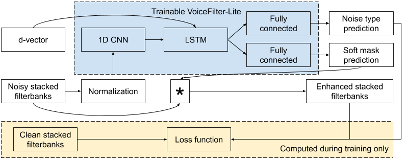
The new VoiceFilter-Lite system has been carefully designed to fit on-device applications. Instead of processing audio waveforms, VoiceFilter-Lite takes exactly the same input features as the speech recognition model (stacked log Mel-filterbanks), and directly enhances these features by filtering out components not belonging to the target speaker in real time. Together with several optimizations on network topologies, the number of runtime operations is drastically reduced. After quantizing the neural network with the TensorFlow Lite library, the model size is only 2.2 MB, which fits most on-device applications.

To train the VoiceFilter-Lite model, the filterbanks of the noisy speech are fed as input to the network together with an embedding vector that represents the identity of the target speaker (i.e., a d-vector). The network predicts a mask that is element-wise multiplied to the input to produce enhanced filterbanks. A loss function is defined to minimize the difference between the enhanced filterbanks and the filterbanks from the clean speech during training.

Model architecture of the VoiceFilter-Lite system.

VoiceFilter-Lite is a plug-and-play model, which allows the application in which it’s implemented to easily bypass it if the speaker did not enroll their voice. This also means that the speech recognition model and the VoiceFilter-Lite model can be separately trained and updated, which largely reduces engineering complexity in the deployment process.

As a plug-and-play model, VoiceFilter-Lite can be easily bypassed if the speaker did not enroll their voice.

Addressing the Challenge of Over-Suppression
When speech separation models are used for improving speech recognition, two types of error could occur: under-suppression, when the model fails to filter out noisy components from the signal; and over-suppression, when the model fails to preserve useful signal, resulting in some words being dropped from the recognized text. Over-suppression is especially problematic since modern speech recognition models are usually already trained with extensively augmented data (such as room simulation and SpecAugment), and thus are more robust to under-suppression.

VoiceFilter-Lite addresses the over-suppression issue with two novel approaches. First, it uses an asymmetric loss during the training process, such that the model is less tolerant to over-suppression than under-suppression. Second, it predicts the type of noise at runtime, and adaptively adjusts the suppression strength according to this prediction.

VoiceFilter-Lite adaptively applies stronger suppression strength when overlapping speech is detected.

With these two solutions, the VoiceFilter-Lite model retains great performance on streaming speech recognition for other scenarios, such as single-speaker speech under quiet or various noise conditions, while still providing significant improvement on overlapping speech. From our experiments, we observed a 25.1% improvement of word error rate after the 2.2MB VoiceFilter-Lite model is applied on additive overlapping speech. For reverberant overlapping speech, which is a more challenging task to simulate far-field devices such as smart home speakers, we also observed a 14.7% improvement of word error rate with VoiceFilter-Lite.

Future Work
While VoiceFilter-Lite has shown great promise for various on-device speech applications, we are also exploring several other directions to make VoiceFilter-Lite more useful. First, our current model is trained and evaluated with English speech only. We are excited about adopting the same technology to improve speech recognition for more languages. Second, we would like to directly optimize the speech recognition loss during the training of VoiceFilter-Lite, which can potentially further improve speech recognition beyond overlapping speech.

Acknowledgements
The research described in this post represents joint efforts from multiple teams within Google. Contributors include Quan Wang, Ignacio Lopez Moreno, Mert Saglam, Kevin Wilson, Alan Chiao, Renjie Liu, Yanzhang He, Wei Li, Jason Pelecanos, Philip Chao, Sinan Akay, John Han, Stephen Wu, Hannah Muckenhirn, Ye Jia, Zelin Wu, Yiteng Huang, Marily Nika, Jaclyn Konzelmann, Nino Tasca, and Alexander Gruenstein.

Source: Google AI Blog


Announcing the Objectron Dataset

The state of the art in machine learning (ML) has achieved exceptional accuracy on many computer vision tasks solely by training models on photos. Building upon these successes and advancing 3D object understanding has great potential to power a wider range of applications, such as augmented reality, robotics, autonomy, and image retrieval. For example, earlier this year we released MediaPipe Objectron, a set of real-time 3D object detection models designed for mobile devices, which were trained on a fully annotated, real-world 3D dataset, that can predict objects’ 3D bounding boxes.

Yet, understanding objects in 3D remains a challenging task due to the lack of large real-world datasets compared to 2D tasks (e.g., ImageNet, COCO, and Open Images). To empower the research community for continued advancement in 3D object understanding, there is a strong need for the release of object-centric video datasets, which capture more of the 3D structure of an object, while matching the data format used for many vision tasks (i.e., video or camera streams), to aid in the training and benchmarking of machine learning models.

Today, we are excited to release the Objectron dataset, a collection of short, object-centric video clips capturing a larger set of common objects from different angles. Each video clip is accompanied by AR session metadata that includes camera poses and sparse point-clouds. The data also contain manually annotated 3D bounding boxes for each object, which describe the object’s position, orientation, and dimensions. The dataset consists of 15K annotated video clips supplemented with over 4M annotated images collected from a geo-diverse sample (covering 10 countries across five continents).

Example videos in the Objectron dataset.

A 3D Object Detection Solution
Along with the dataset, we are also sharing a 3D object detection solution for four categories of objects — shoes, chairs, mugs, and cameras. These models are released in MediaPipe, Google's open source framework for cross-platform customizable ML solutions for live and streaming media, which also powers ML solutions like on-device real-time hand, iris and body pose tracking.

Sample results of 3D object detection solution running on mobile.

In contrast to the previously released single-stage Objectron model, these newest versions utilize a two-stage architecture. The first stage employs the TensorFlow Object Detection model to find the 2D crop of the object. The second stage then uses the image crop to estimate the 3D bounding box while simultaneously computing the 2D crop of the object for the next frame, so that the object detector does not need to run every frame. The second stage 3D bounding box predictor runs at 83 FPS on Adreno 650 mobile GPU.

Diagram of a reference 3D object detection solution.

Evaluation Metric for 3D Object Detection
With ground truth annotations, we evaluate the performance of 3D object detection models using 3D intersection over union (IoU) similarity statistics, a commonly used metric for computer vision tasks, which measures how close the bounding boxes are to the ground truth.

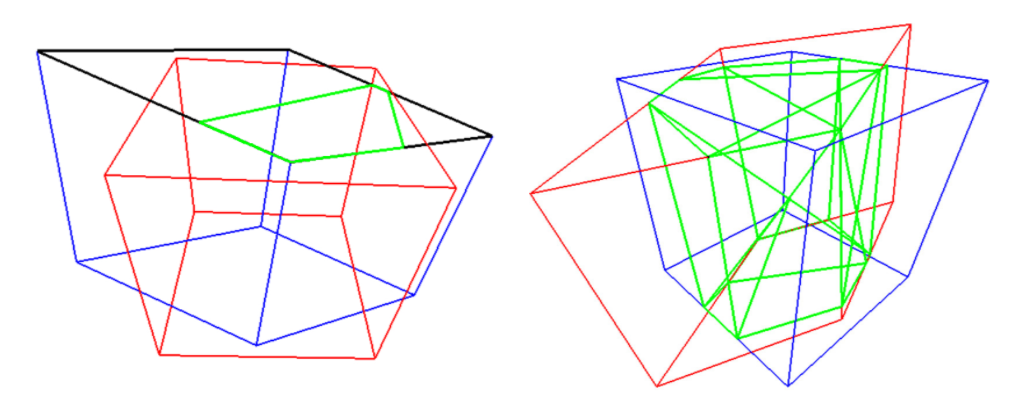
We propose an algorithm for computing accurate 3D IoU values for general 3D-oriented boxes. First, we compute the intersection points between faces of the two boxes using Sutherland-Hodgman Polygon clipping algorithm. This is similar to frustum culling, a technique used in computer graphics. The volume of the intersection is computed by the convex hull of all the clipped polygons. Finally, the IoU is computed from the volume of the intersection and volume of the union of two boxes. We are releasing the evaluation metrics source code along with the dataset.

Compute the 3D intersection over union using the polygon clipping algorithm, Left: Compute the intersection points of each face by clipping the polygon against the box. Right: Compute the volume of intersection by computing the convex hull of all intersection points (green).

Dataset Format
The technical details of the Objectron dataset, including usage and tutorials, are available on the dataset website. The dataset includes bikes, books, bottles, cameras, cereal boxes, chairs, cups, laptops, and shoes, and is stored in the objectron bucket on Google Cloud storage with the following assets:

  • The video sequences
  • The annotation labels (3D bounding boxes for objects)
  • AR metadata (such as camera poses, point clouds, and planar surfaces)
  • Processed dataset: shuffled version of the annotated frames, in tf.example format for images and SequenceExample format for videos.
  • Supporting scripts to run evaluation based on the metric described above
  • Supporting scripts to load the data into Tensorflow, PyTorch, and Jax and to visualize the dataset, including “Hello World” examples

With the dataset, we are also open-sourcing a data-pipeline to parse the dataset in popular Tensorflow, PyTorch and Jax frameworks. Example colab notebooks are also provided.

By releasing this Objectron dataset, we hope to enable the research community to push the limits of 3D object geometry understanding. We also hope to foster new research and applications, such as view synthesis, improved 3D representation, and unsupervised learning. Stay tuned for future activities and developments by joining our mailing list and visiting our github page.

Acknowledgements
The research described in this post was done by Adel Ahmadyan, Liangkai Zhang, Jianing Wei, Artsiom Ablavatski, Mogan Shieh, Ryan Hickman, Buck Bourdon, Alexander Kanaukou, Chuo-Ling Chang, Matthias Grundmann, ‎and Tom Funkhouser. We thank Aliaksandr Shyrokau, Sviatlana Mialik, Anna Eliseeva, and the annotation team for their high quality annotations. We also would like to thank Jonathan Huang and Vivek Rathod for their guidance on TensorFlow Object Detection API.

Source: Google AI Blog


Background Features in Google Meet, Powered by Web ML

Video conferencing is becoming ever more critical in people's work and personal lives. Improving that experience with privacy enhancements or fun visual touches can help center our focus on the meeting itself. As part of this goal, we recently announced ways to blur and replace your background in Google Meet, which use machine learning (ML) to better highlight participants regardless of their surroundings. Whereas other solutions require installing additional software, Meet’s features are powered by cutting-edge web ML technologies built with MediaPipe that work directly in your browser — no extra steps necessary. One key goal in developing these features was to provide real-time, in-browser performance on almost all modern devices, which we accomplished by combining efficient on-device ML models, WebGL-based rendering, and web-based ML inference via XNNPACK and TFLite.

Background blur and background replacement, powered by MediaPipe on the web.

Overview of Our Web ML Solution
The new features in Meet are developed with MediaPipe, Google's open source framework for cross-platform customizable ML solutions for live and streaming media, which also powers ML solutions like on-device real-time hand, iris and body pose tracking.

A core need for any on-device solution is to achieve high performance. To accomplish this, MediaPipe’s web pipeline leverages WebAssembly, a low-level binary code format designed specifically for web browsers that improves speed for compute-heavy tasks. At runtime, the browser converts WebAssembly instructions into native machine code that executes much faster than traditional JavaScript code. In addition, Chrome 84 recently introduced support for WebAssembly SIMD, which processes multiple data points with each instruction, resulting in a performance boost of more than 2x.

Our solution first processes each video frame by segmenting a user from their background (more about our segmentation model later in the post) utilizing ML inference to compute a low resolution mask. Optionally, we further refine the mask to align it with the image boundaries. The mask is then used to render the video output via WebGL2, with the background blurred or replaced.

WebML Pipeline: All compute-heavy operations are implemented in C++/OpenGL and run within the browser via WebAssembly.

In the current version, model inference is executed on the client’s CPU for low power consumption and widest device coverage. To achieve real-time performance, we designed efficient ML models with inference accelerated by the XNNPACK library, the first inference engine specifically designed for the novel WebAssembly SIMD specification. Accelerated by XNNPACK and SIMD, the segmentation model can run in real-time on the web.

Enabled by MediaPipe's flexible configuration, the background blur/replace solution adapts its processing based on device capability. On high-end devices it runs the full pipeline to deliver the highest visual quality, whereas on low-end devices it continues to perform at speed by switching to compute-light ML models and bypassing the mask refinement.

Segmentation Model
On-device ML models need to be ultra lightweight for fast inference, low power consumption, and small download size. For models running in the browser, the input resolution greatly affects the number of floating-point operations (FLOPs) necessary to process each frame, and therefore needs to be small as well. We downsample the image to a smaller size before feeding it to the model. Recovering a segmentation mask as fine as possible from a low-resolution image adds to the challenges of model design.

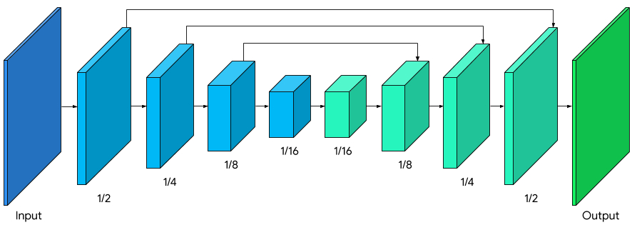
The overall segmentation network has a symmetric structure with respect to encoding and decoding, while the decoder blocks (light green) also share a symmetric layer structure with the encoder blocks (light blue). Specifically, channel-wise attention with global average pooling is applied in both encoder and decoder blocks, which is friendly to efficient CPU inference.

Model architecture with MobileNetV3 encoder (light blue), and a symmetric decoder (light green).

We modified MobileNetV3-small as the encoder, which has been tuned by network architecture search for the best performance with low resource requirements. To reduce the model size by 50%, we exported our model to TFLite using float16 quantization, resulting in a slight loss in weight precision but with no noticeable effect on quality. The resulting model has 193K parameters and is only 400KB in size.

Rendering Effects
Once segmentation is complete, we use OpenGL shaders for video processing and effect rendering, where the challenge is to render efficiently without introducing artifacts. In the refinement stage, we apply a joint bilateral filter to smooth the low resolution mask.

Rendering effects with artifacts reduced. Left: Joint bilateral filter smooths the segmentation mask. Middle: Separable filters remove halo artifacts in background blur. Right: Light wrapping in background replace.

The blur shader simulates a bokeh effect by adjusting the blur strength at each pixel proportionally to the segmentation mask values, similar to the circle-of-confusion (CoC) in optics. Pixels are weighted by their CoC radii, so that foreground pixels will not bleed into the background. We implemented separable filters for the weighted blur, instead of the popular Gaussian pyramid, as it removes halo artifacts surrounding the person. The blur is performed at a low resolution for efficiency, and blended with the input frame at the original resolution.

Background blur examples.

For background replacement, we adopt a compositing technique, known as light wrapping, for blending segmented persons and customized background images. Light wrapping helps soften segmentation edges by allowing background light to spill over onto foreground elements, making the compositing more immersive. It also helps minimize halo artifacts when there is a large contrast between the foreground and the replaced background.

Background replacement examples.

Performance
To optimize the experience for different devices, we provide model variants at multiple input sizes (i.e., 256x144 and 160x96 in the current release), automatically selecting the best according to available hardware resources.

We evaluated the speed of model inference and the end-to-end pipeline on two common devices: MacBook Pro 2018 with 2.2 GHz 6-Core Intel Core i7, and Acer Chromebook 11 with Intel Celeron N3060. For 720p input, the MacBook Pro can run the higher-quality model at 120 FPS and the end-to-end pipeline at 70 FPS, while the Chromebook runs inference at 62 FPS with the lower-quality model and 33 FPS end-to-end.

 Model   FLOPs   Device   Model Inference   Pipeline 
 256x144   64M   MacBook Pro 18   8.3ms (120 FPS)   14.3ms (70 FPS) 
 160x96   27M   Acer Chromebook 11   16.1ms (62 FPS)   30ms (33 FPS) 
Model inference speed and end-to-end pipeline on high-end (MacBook Pro) and low-end (Chromebook) laptops.

For quantitative evaluation of model accuracy, we adopt the popular metrics of intersection-over-union (IOU) and boundary F-measure. Both models achieve high quality, especially for having such a lightweight network:

  Model     IOU     Boundary  
  F-measure  
  256x144     93.58%     0.9024  
  160x96     90.79%     0.8542  
Evaluation of model accuracy, measured by IOU and boundary F-score.

We also release the accompanying Model Card for our segmentation models, which details our fairness evaluations. Our evaluation data contains images from 17 geographical subregions of the globe, with annotations for skin tone and gender. Our analysis shows that the model is consistent in its performance across the various regions, skin-tones, and genders, with only small deviations in IOU metrics.

Conclusion
We introduced a new in-browser ML solution for blurring and replacing your background in Google Meet. With this, ML models and OpenGL shaders can run efficiently on the web. The developed features achieve real-time performance with low power consumption, even on low-power devices.

Acknowledgments
Special thanks to those on the Meet team and others who worked on this project, in particular Sebastian Jansson, Rikard Lundmark, Stephan Reiter, Fabian Bergmark, Ben Wagner, Stefan Holmer, Dan Gunnarson, Stéphane Hulaud and to all our team members who worked on the technology with us: Siargey Pisarchyk, Karthik Raveendran, Chris McClanahan, Marat Dukhan, Frank Barchard, Ming Guang Yong, Chuo-Ling Chang, Michael Hays, Camillo Lugaresi, Gregory Karpiak, Siarhei Kazakou, Matsvei Zhdanovich, and Matthias Grundmann.

Source: Google AI Blog


Recreating Historical Streetscapes Using Deep Learning and Crowdsourcing

For many, gazing at an old photo of a city can evoke feelings of both nostalgia and wonder — what was it like to walk through Manhattan in the 1940s? How much has the street one grew up on changed? While Google Street View allows people to see what an area looks like in the present day, what if you want to explore how places looked in the past?

To create a rewarding “time travel” experience for both research and entertainment purposes, we are launching (pronounced as re”turn"), an open source, scalable system running on Google Cloud and Kubernetes that can reconstruct cities from historical maps and photos, representing an implementation of our suite of open source tools launched earlier this year. Referencing the common prefix meaning again or anew, is meant to represent the themes of reconstruction, research, recreation and remembering behind this crowdsourced research effort, and consists of three components:

  • A crowdsourcing platform, which allows users to upload historical maps of cities, georectify (i.e., match them to real world coordinates), and vectorize them
  • A temporal map server, which shows how maps of cities change over time
  • A 3D experience platform, which runs on top of the map server, creating the 3D experience by using deep learning to reconstruct buildings in 3D from limited historical images and maps data.

Our goal is for to become a compendium that allows history enthusiasts to virtually experience historical cities around the world, aids researchers, policy makers and educators, and provides a dose of nostalgia to everyday users.

Bird’s eye view of Chelsea, Manhattan with a time slider from 1890 to 1970, crafted from historical photos and maps and using ’s 3D reconstruction pipeline and colored with a preset Manhattan-inspired palette.

Crowdsourcing Data from Historical Maps
Reconstructing how cities used to look at scale is a challenge — historical image data is more difficult to work with than modern data, as there are far fewer images available and much less metadata captured from the images. To help with this difficulty, the maps module is a suite of open source tools that work together to create a map server with a time dimension, allowing users to jump back and forth between time periods using a slider. These tools allow users to upload scans of historical print maps, georectify them to match real world coordinates, and then convert them to vector format by tracing their geographic features. These vectorized maps are then served on a tile server and rendered as slippy maps, which lets the user zoom in and pan around.

Sub-modules of the suite of tools

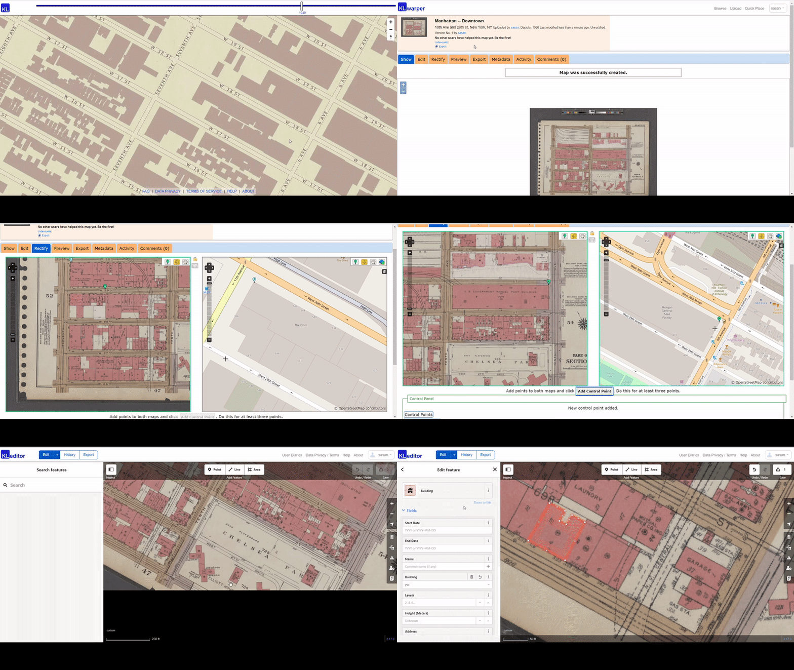
The entry point of the maps module is Warper, a web app that allows users to upload historical images of maps and georectify them by finding control points on the historical map and corresponding points on a base map. The next app, Editor, allows users to load the georectified historical maps as the background and then trace their geographic features (e.g., building footprints, roads, etc.). This traced data is stored in an OpenStreetMap (OSM) vector format. They are then converted to vector tiles and served from the Server app, a vector tile server. Finally, our map renderer, Kartta, visualizes the spatiotemporal vector tiles allowing the users to navigate space and time on historical maps. These tools were built on top of numerous open source resources including OpenStreetMap, and we intend for our tools and data to be completely open source as well.

Warper and Editor work together to let users upload a map, anchor it to a base map using control points, and trace geographic features like building footprints and roads.

3D Experience
The 3D Models module aims to reconstruct the detailed full 3D structures of historical buildings using the associated images and maps data, organize these 3D models properly in one repository, and render them on the historical maps with a time dimension.

In many cases, there is only one historical image available for a building, which makes the 3D reconstruction an extremely challenging problem. To tackle this challenge, we developed a coarse-to-fine reconstruction-by-recognition algorithm.

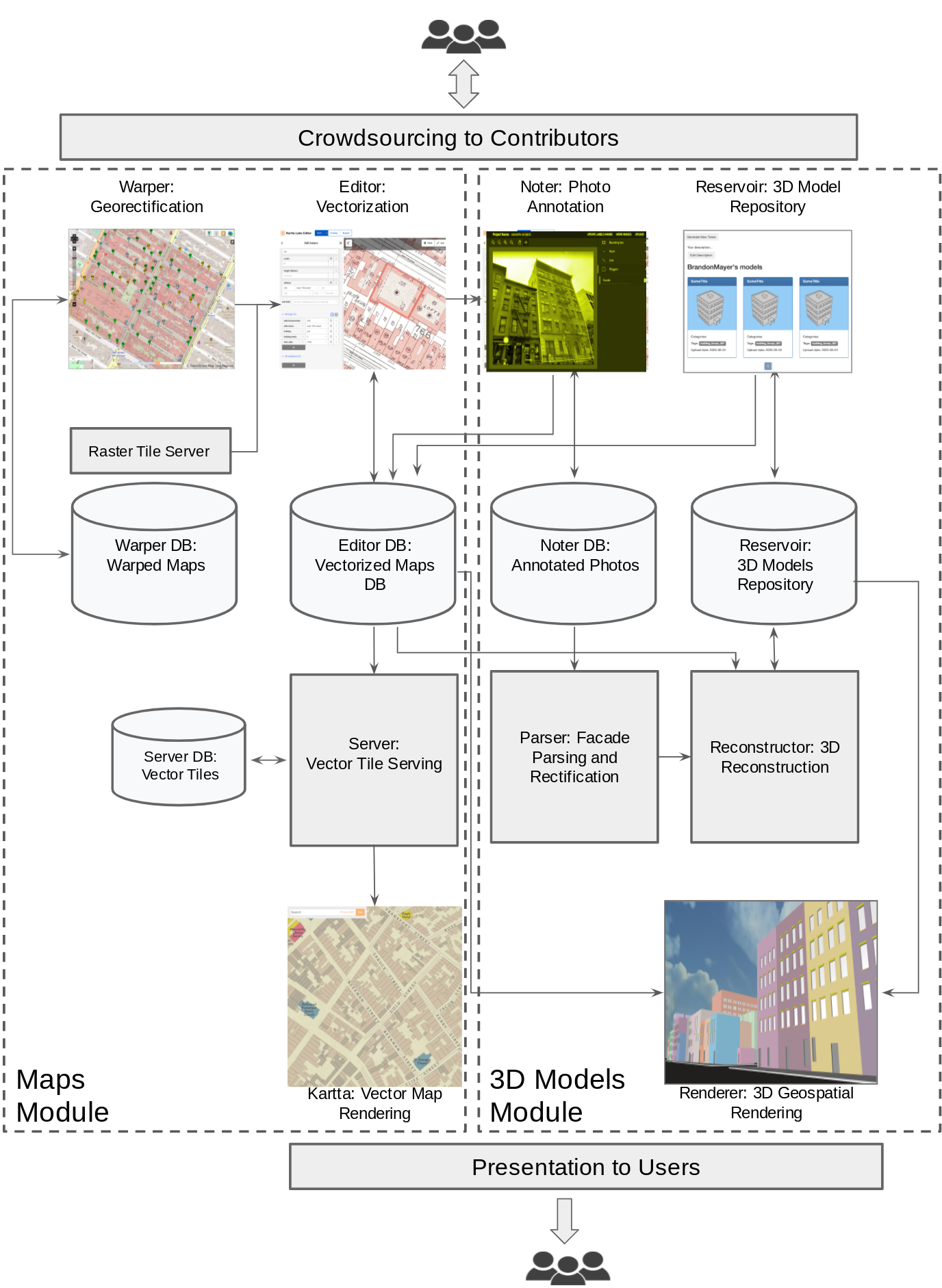
High-level overview of ’s 3D reconstruction pipeline, which takes annotated images and maps and prepares them for 3D rendering.

Starting with footprints on maps and façade regions in historical images (both are annotated by crowdsourcing or detected by automatic algorithms), the footprint of one input building is extruded upwards to generate its coarse 3D structure. The height of this extrusion is set to the number of floors from the corresponding metadata in the maps database.

In parallel, instead of directly inferring the detailed 3D structures of each façade as one entity, the 3D reconstruction pipeline recognizes all individual constituent components (e.g., windows, entries, stairs, etc.) and reconstructs their 3D structures separately based on their categories. Then these detailed 3D structures are merged with the coarse one for the final 3D mesh. The results are stored in a 3D repository and ready for 3D rendering.

The key technology powering this feature is a number of state-of-art deep learning models:

  • Faster region-based convolutional neural networks (RCNN) were trained using the façade component annotations for each target semantic class (e.g., windows, entries, stairs, etc), which are used to localize bounding-box level instances in historical images.
  • DeepLab, a semantic segmentation model, was trained to provide pixel-level labels for each semantic class.
  • A specifically designed neural network was trained to enforce high-level regularities within the same semantic class. This ensured that windows generated on a façade were equally spaced and consistent in shape with each other. This also facilitated consistency across different semantic classes such as stairs to ensure they are placed at reasonable positions and have consistent dimensions relative to the associated entry ways.

Key Results

Street level view of 3D-reconstructed Chelsea, Manhattan

Conclusion
With , we have developed tools that facilitate crowdsourcing to tackle the main challenge of insufficient historical data when recreating virtual cities. The 3D experience is still a work-in-progress and we aim to improve it with future updates. We hope acts as a nexus for an active community of enthusiasts and casual users that not only utilizes our historical datasets and open source code, but actively contributes to both.

Acknowledgements
This effort has been successful thanks to the hard work of many people, including, but not limited to the following (in alphabetical order of last name): Yale Cong, Feng Han, Amol Kapoor, Raimondas Kiveris, Brandon Mayer, Mark Phillips, Sasan Tavakkol, and Tim Waters (Waters Geospatial Ltd).

Source: Google AI Blog


Advancing NLP with Efficient Projection-Based Model Architectures

Deep neural networks have radically transformed natural language processing (NLP) in the last decade, primarily through their application in data centers using specialized hardware. However, issues such as preserving user privacy, eliminating network latency, enabling offline functionality, and reducing operation costs have rapidly spurred the development of NLP models that can be run on-device rather than in data centers. Yet mobile devices have limited memory and processing power, which requires models running on them to be small and efficient — without compromising quality.

Last year, we published a neural architecture called PRADO, which at the time achieved state-of-the-art performance on many text classification problems, using a model with less than 200K parameters. While most models use a fixed number of parameters per token, the PRADO model used a network structure that required extremely few parameters to learn the most relevant or useful tokens for the task.

Today we describe a new extension to the model, called pQRNN, which advances the state of the art for NLP performance with a minimal model size. The novelty of pQRNN is in how it combines a simple projection operation with a quasi-RNN encoder for fast, parallel processing. We show that the pQRNN model is able to achieve BERT-level performance on a text classification task with orders of magnitude fewer number of parameters.

What Makes PRADO Work?
When developed a year ago, PRADO exploited NLP domain-specific knowledge on text segmentation to reduce the model size and improve the performance. Normally, the text input to NLP models is first processed into a form that is suitable for the neural network, by segmenting text into pieces (tokens) that correspond to values in a predefined universal dictionary (a list of all possible tokens). The neural network then uniquely identifies each segment using a trainable parameter vector, which comprises the embedding table. However, the way in which text is segmented has a significant impact on the model performance, size, and latency. The figure below shows the spectrum of approaches used by the NLP community and their pros and cons.

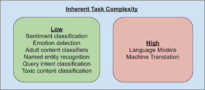
Since the number of text segments is such an important parameter for model performance and compression, it raises the question of whether or not an NLP model needs to be able to distinctly identify every possible text segment. To answer this question we look at the inherent complexity of NLP tasks.

Only a few NLP tasks (e.g., language models and machine translation) need to know subtle differences between text segments and thus need to be capable of uniquely identifying all possible text segments. In contrast, the majority of other tasks can be solved by knowing a small subset of these segments. Furthermore, this subset of task-relevant segments will likely not be the most frequent, as a significant fraction of segments will undoubtedly be dedicated to articles, such as a, an, the, etc., which for many tasks are not necessarily critical. Hence, allowing the network to determine the most relevant segments for a given task results in better performance. In addition, the network does not need to be able to uniquely identify these segments, but only needs to recognize clusters of text segments. For example, a sentiment classifier just needs to know segment clusters that are strongly correlated to the sentiment in the text.

Leveraging these insights, PRADO was designed to learn clusters of text segments from words rather than word pieces or characters, which enabled it to achieve good performance on low-complexity NLP tasks. Since word units are more meaningful, and yet the most relevant words for most tasks are reasonably small, many fewer model parameters are needed to learn such a reduced subset of relevant word clusters.

Improving PRADO
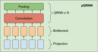
Building on the success of PRADO, we developed an improved NLP model, called pQRNN. This model is composed of three building blocks, a projection operator that converts tokens in text to a sequence of ternary vectors, a dense bottleneck layer and a stack of QRNN encoders.

The implementation of the projection layer in pQRNN is identical to that used in PRADO and helps the model learn the most relevant tokens without a fixed set of parameters to define them. It first fingerprints the tokens in the text and converts it to a ternary feature vector using a simple mapping function. This results in a ternary vector sequence with a balanced symmetric distribution that uniquely represents the text. This representation is not directly useful since it does not have any information needed to solve the task of interest and the network has no control over this representation. We combine it with a dense bottleneck layer to allow the network to learn a per word representation that is relevant for the task at hand. The representation resulting from the bottleneck layer still does not take the context of the word into account. We learn a contextual representation by using a stack of bidirectional QRNN encoders. The result is a network that is capable of learning a contextual representation from just text input without employing any kind of preprocessing.

Performance
We evaluated pQRNN on the civil_comments dataset and compared it with the BERT model on the same task. Simply because the model size is proportional to the number of parameters, pQRNN is much smaller than BERT. But in addition, pQRNN is quantized, further reducing the model size by a factor of 4x. The public pretrained version of BERT performed poorly on the task hence the comparison is done to a BERT version that is pretrained on several different relevant multilingual data sources to achieve the best possible performance.

We capture the area under the curve (AUC) for the two models. Without any kind of pre-training and just trained on the supervised data, the AUC for pQRNN is 0.963 using 1.3 million quantized (8-bit) parameters. With pre-training on several different data sources and fine-tuning on the supervised data, the BERT model gets 0.976 AUC using 110 million floating point parameters.

Conclusion
Using our previous generation model PRADO, we have demonstrated how it can be used as the foundation for the next generation of state-of-the-art light-weight text classification models. We present one such model, pQRNN, and show that this new architecture can nearly achieve BERT-level performance, despite using 300x fewer parameters and being trained on only the supervised data. To stimulate further research in this area, we have open-sourced the PRADO model and encourage the community to use it as a jumping off point for new model architectures.

Acknowledgements
We thank Yicheng Fan, Márius Šajgalík, Peter Young and Arun Kandoor for contributing to the open sourcing effort and helping improve the models. We would also like to thank Amarnag Subramanya, Ashwini Venkatesh, Benoit Jacob, Catherine Wah, Dana Movshovitz-Attias, Dang Hien, Dmitry Kalenichenko, Edgar Gonzàlez i Pellicer, Edward Li, Erik Vee, Evgeny Livshits, Gaurav Nemade, Jeffrey Soren, Jeongwoo Ko, Julia Proskurnia, Rushin Shah, Shirin Badiezadegan, Sidharth KV, Victor Cărbune and the Learn2Compress team for their support. We would like to thank Andrew Tomkins and Patrick Mcgregor for sponsoring this research project.

Source: Google AI Blog