Posted by Mike Schuster (Google Brain Team), Melvin Johnson (Google Translate) and Nikhil Thorat (Google Brain Team)
In the last 10 years, Google Translate has grown from supporting just a few languages to 103, translating over 140 billion words every day. To make this possible, we needed to build and maintain many different systems in order to translate between any two languages, incurring significant computational cost. With neural networks reforming many fields, we were convinced we could raise the translation quality further, but doing so would mean rethinking the technology behind Google Translate.
In September, we announced that Google Translate is switching to a new system called Google Neural Machine Translation (GNMT), an end-to-end learning framework that learns from millions of examples, and provided significant improvements in translation quality. However, while switching to GNMT improved the quality for the languages we tested it on, scaling up to all the 103 supported languages presented a significant challenge.
In “Google’s Multilingual Neural Machine Translation System: Enabling Zero-Shot Translation”, we address this challenge by extending our previous GNMT system, allowing for a single system to translate between multiple languages. Our proposed architecture requires no change in the base GNMT system, but instead uses an additional “token” at the beginning of the input sentence to specify the required target language to translate to. In addition to improving translation quality, our method also enables “Zero-Shot Translation” — translation between language pairs never seen explicitly by the system.
Here’s how it works. Let’s say we train a multilingual system with Japanese⇄English and Korean⇄English examples, shown by the solid blue lines in the animation. Our multilingual system, with the same size as a single GNMT system, shares its parameters to translate between these four different language pairs. This sharing enables the system to transfer the “translation knowledge” from one language pair to the others. This transfer learning and the need to translate between multiple languages forces the system to better use its modeling power.
This inspired us to ask the following question: Can we translate between a language pair which the system has never seen before? An example of this would be translations between Korean and Japanese where Korean⇄Japanese examples were not shown to the system. Impressively, the answer is yes — it can generate reasonable Korean⇄Japanese translations, even though it has never been taught to do so. We call this “zero-shot” translation, shown by the yellow dotted lines in the animation. To the best of our knowledge, this is the first time this type of transfer learning has worked in Machine Translation.
The success of the zero-shot translation raises another important question: Is the system learning a common representation in which sentences with the same meaning are represented in similar ways regardless of language — i.e. an “interlingua”? Using a 3-dimensional representation of internal network data, we were able to take a peek into the system as it translates a set of sentences between all possible pairs of the Japanese, Korean, and English languages.
Part (a) from the figure above shows an overall geometry of these translations. The points in this view are colored by the meaning; a sentence translated from English to Korean with the same meaning as a sentence translated from Japanese to English share the same color. From this view we can see distinct groupings of points, each with their own color. Part (b) zooms in to one of the groups, and part (c) colors by the source language. Within a single group, we see a sentence with the same meaning but from three different languages. This means the network must be encoding something about the semantics of the sentence rather than simply memorizing phrase-to-phrase translations. We interpret this as a sign of existence of an interlingua in the network.
We show many more results and analyses in our paper, and hope that its findings are not only interesting for machine learning or machine translation researchers but also to linguists and others who are interested in how multiple languages can be processed by machines using a single system.
Finally, the described Multilingual Google Neural Machine Translation system is running in production today for all Google Translate users. Multilingual systems are currently used to serve 10 of the recently launched 16 language pairs, resulting in improved quality and a simplified production architecture.
It has been an eventful year since the Google Brain Teamopen-sourced TensorFlow to accelerate machine learning research and make technology work better for everyone. There has been an amazing amount of activity around the project: more than 480 people have contributed directly to TensorFlow, including Googlers, external researchers, independent programmers, students, and senior developers at other large companies. TensorFlow is now the most popular machine learning project on GitHub.
We’re especially excited to see how people all over the world are using TensorFlow. For example:
Australian marine biologists are using TensorFlow to find sea cows in tens of thousands of hi-res photos to better understand their populations, which are under threat of extinction.
An enterprising Japanese cucumber farmer trained a model with TensorFlow to sort cucumbers by size, shape, and other characteristics.
Data scientists in the Bay Area have rigged up TensorFlow and the Raspberry Pi to keep track of the Caltrain.
We’re committed to making sure TensorFlow scales all the way from research to production and from the tiniest Raspberry Pi all the way up to server farms filled with GPUs or TPUs. But TensorFlow is more than a single open-source project – we’re doing our best to foster an open-source ecosystem of related software and machine learning models around it:
The TensorFlow Serving project simplifies the process of serving TensorFlow models in production.
TensorFlow “Wide and Deep” models combine the strengths of traditional linear models and modern deep neural networks.
For those who are interested in working with TensorFlow in the cloud, Google Cloud Platform recently launched Cloud Machine Learning, which offers TensorFlow as a managed service.
Thanks very much to all of you who have already adopted TensorFlow in your cutting-edge products, your ambitious research, your fast-growing startups, and your school projects; special thanks to everyone who has contributed directly to the codebase. In collaboration with the global machine learning community, we look forward to making TensorFlow even better in the years to come!
Jupyter is a powerful open source technology that gives you a platform to write and execute code to analyze, visualize and share the discoveries you find in your big data set. You can download a number of different Docker images preconfigured with many different notebook extensions and software packages to help you on any kind of data-science quest.
If you’re exploring on your own, and really want to get started quickly, you can get this all running on your local computer, but what if you want to take your expertise and lead a classroom of people along the same path? You have to either configure everything for them or walk them through configuring their own machines with all the required software.
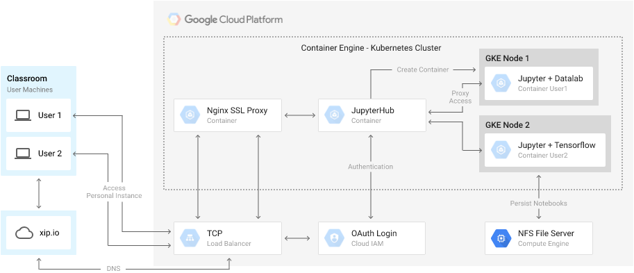
This is where JupyterHub comes in, as a management layer in front of Jupyter instances, allowing you to configure users, using custom authentication, and giving you a Python interface to spawn new Jupyter instances for each user. Even with JupyterHub, you still need a way to provision physical and virtual hardware for the students.
Enter Kubernetes, an open source system for automating deploying, scaling and managing containerized applications. Google Container Engine is a fully managed service based on Kubernetes, allowing you to create clusters easily on Google Cloud Platform.
This solution comes with a JupyterHub Spawner class that allows it to create Kubernetes Pods, which are Docker images running Jupyter, for each user. It also comes with all the automation scripts required to create a Container Engine cluster and let you easily customize your setup.
When your students log into JupyterHub using Google OAuth2, they can choose from a list of several pre-built Jupyter images, including a newly updated “datalab-jupyter” image, which comes with the Google Datalab open source notebook extension enabling integration with BigQuery, Google Cloud ML, StackDriver, and it also has TensorFlow and the Apache Beam Python SDK for Google Cloud DataFlow installed. Users can also choose to run any of the pre-configured Jupyter docker-stack images, or you can build your own Docker images to run any special libraries or Jupyter configurations you want.
We hope that this solution allows you to get your classroom or team environment running quickly so you can focus on learning rather than configuring machines.
Posted by Vincent Dumoulin*, Jonathon Shlens and Manjunath Kudlur, Google Brain Team
Pastiche. A French word, it designates a work of art that imitates the style of another one (not to be confused with its more humorous Greek cousin, parody). Although it has been used for a long time in visual art, music and literature, pastiche has been getting mass attention lately with online forums dedicated to images that have been modified to be in the style of famous paintings. Using a technique known as style transfer, these images are generated by phone or web apps that allow a user to render their favorite picture in the style of a well known work of art.
Although users have already produced gorgeous pastiches using the current technology, we feel that it could be made even more engaging. Right now, each painting is its own island, so to speak: the user provides a content image, selects an artistic style and gets a pastiche back. But what if one could combine many different styles, exploring unique mixtures of well known artists to create an entirely unique pastiche?
Learning a representation for artistic style
In our recent paper titled “A Learned Representation for Artistic Style”, we introduce a simple method to allow a single deep convolutional style transfer network to learn multiple styles at the same time. The network, having learned multiple styles, is able to do style interpolation, where the pastiche varies smoothly from one style to another. Our method enables style interpolation in real-time as well, allowing this to be applied not only to static images, but also videos.
Credit: awesome dog role played by Google Brain team office dog Picabo.
In the video above, multiple styles are combined in real-time and the resulting style is applied using a single style transfer network. The user is provided with a set of 13 different painting styles and adjusts their relative strengths in the final style via sliders. In this demonstration, the user is an active participant in producing the pastiche.
A Quick History of Style Transfer
While transferring the style of one image to another has existed for nearly 15 years [1] [2], leveraging neural networks to accomplish it is both very recent and very fascinating. In “A Neural Algorithm of Artistic Style” [3], researchers Gatys, Ecker & Bethge introduced a method that uses deep convolutional neural network (CNN) classifiers. The pastiche image is found via optimization: the algorithm looks for an image which elicits the same kind of activations in the CNN’s lower layers - which capture the overall rough aesthetic of the style input (broad brushstrokes, cubist patterns, etc.) - yet produces activations in the higher layers - which capture the things that make the subject recognizable - that are close to those produced by the content image. From some starting point (e.g. random noise, or the content image itself), the pastiche image is progressively refined until these requirements are met.
This work is considered a breakthrough in the field of deep learning research because it provided the first proof of concept for neural network-based style transfer. Unfortunately this method for stylizing an individual image is computationally demanding. For instance, in the first demos available on the web, one would upload a photo to a server, and then still have plenty of time to go grab a cup of coffee before a result was available.
This process was sped up significantly by subsequent research [4, 5] that recognized that this optimization problem may be recast as an image transformation problem, where one wishes to apply a single, fixed painting style to an arbitrary content image (e.g. a photograph). The problem can then be solved by teaching a feed-forward, deep convolutional neural network to alter a corpus of content images to match the style of a painting. The goal of the trained network is two-fold: maintain the content of the original image while matching the visual style of the painting.
The end result of this was that what once took a few minutes for a single static image, could now be run real time (e.g. applying style transfer to a live video). However, the increase in speed that allowed real-time style transfer came with a cost - a given style transfer network is tied to the style of a single painting, losing some flexibility of the original algorithm, which was not tied to any one style. This means that to build a style transfer system capable of modeling 100 paintings, one has to train and store 100 separate style transfer networks.
Our Contribution: Learning and Combining Multiple Styles
We started from the observation that many artists from the impressionist period employ similar brush stroke techniques and color palettes. Furthermore, painting by say, Monet, are even more visually similar.
We leveraged this observation in our training of a machine learning system. That is, we trained a single system that is able to capture and generalize across many Monet paintings or even a diverse array of artists across genres. The pastiches produced are qualitatively comparable to those produced in previous work, while originating from the same style transfer network.
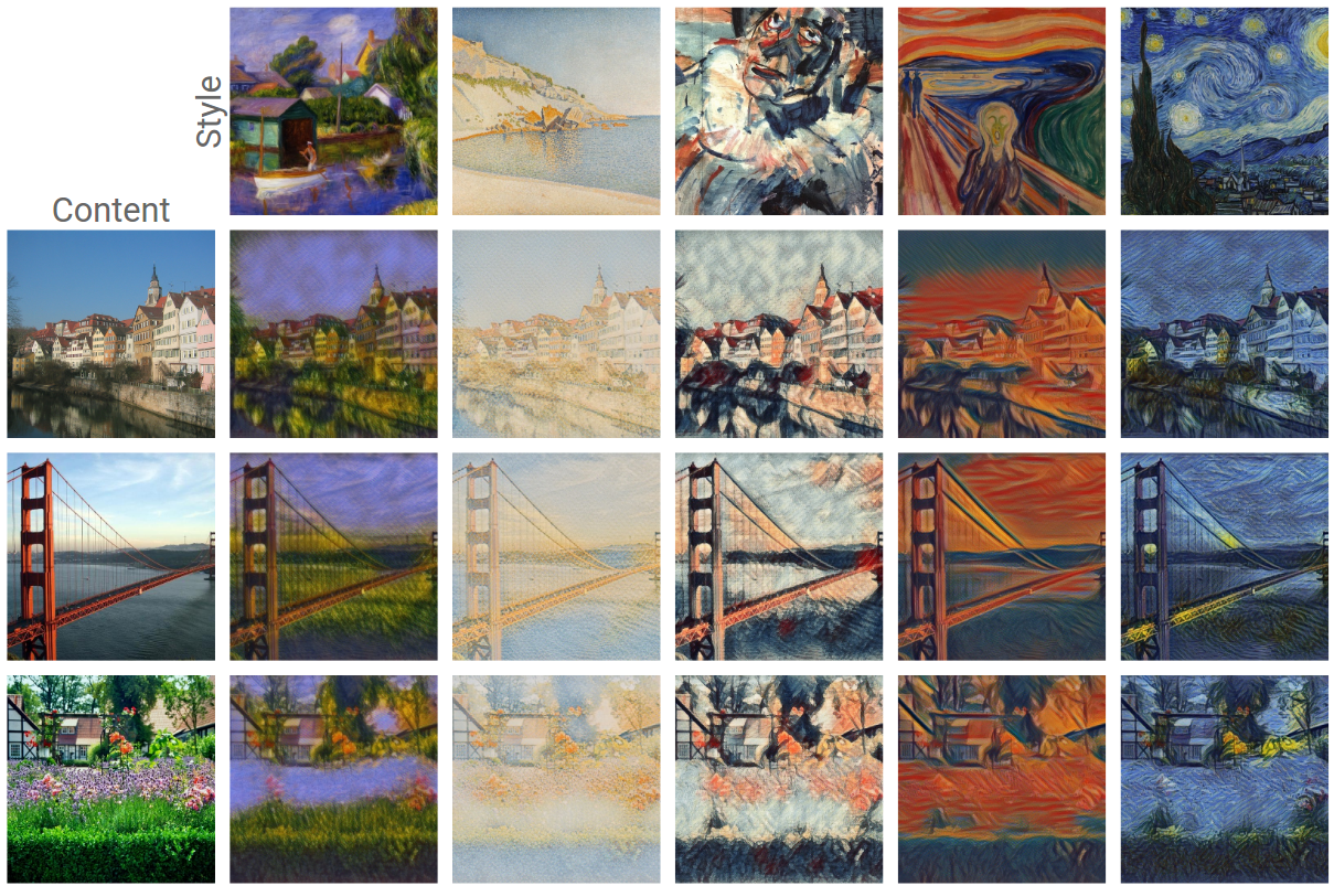
The technique we developed is simple to implement and is not memory intensive. Furthermore, our network, trained on several artistic styles, permits arbitrary combining multiple painting styles in real-time, as shown in the video above. Here are four styles being combined in different proportions on a photograph of Tübingen:
Unlike previous approaches to fast style transfer, we feel that this method of modeling multiple styles at the same time opens the door to exciting new ways for users to interact with style transfer algorithms, not only allowing the freedom to create new styles based on the mixture of several others, but to do it in real-time. Stay tuned for a future post on the Magenta blog, in which we will describe the algorithm in more detail and release the TensorFlow source code to run this model and demo yourself. We also recommend that you check out Nat & Lo’s fantastic video explanation on the subject of style transfer.
Posted by Nick Johnston and David Minnen, Software Engineers
Data compression is used nearly everywhere on the internet - the videos you watch online, the images you share, the music you listen to, even the blog you're reading right now. Compression techniques make sharing the content you want quick and efficient. Without data compression, the time and bandwidth costs for getting the information you need, when you need it, would be exorbitant!
We introduce an architecture that uses a new variant of the Gated Recurrent Unit (a type of RNN that allows units to save activations and process sequences) called Residual Gated Recurrent Unit (Residual GRU). Our Residual GRU combines existing GRUs with the residual connections introduced in "Deep Residual Learning for Image Recognition" to achieve significant image quality gains for a given compression rate. Instead of using a DCT to generate a new bit representation like many compression schemes in use today, we train two sets of neural networks - one to create the codes from the image (encoder) and another to create the image from the codes (decoder).
Our system works by iteratively refining a reconstruction of the original image, with both the encoder and decoder using Residual GRU layers so that additional information can pass from one iteration to the next. Each iteration adds more bits to the encoding, which allows for a higher quality reconstruction. Conceptually, the network operates as follows:
The initial residual, R[0], corresponds to the original image I: R[0] = I.
Set i=1 for to the first iteration.
Iteration[i] takes R[i-1] as input and runs the encoder and binarizer to compress the image into B[i].
Iteration[i] runs the decoder on B[i] to generate a reconstructed image P[i].
The residual for Iteration[i] is calculated: R[i] = I - P[i].
Set i=i+1 and go to Step 3 (up to the desired number of iterations).
The residual image represents how different the current version of the compressed image is from the original. This image is then given as input to the network with the goal of removing the compression errors from the next version of the compressed image. The compressed image is now represented by the concatenation of B[1] through B[N]. For larger values of N, the decoder gets more information on how to reduce the errors and generate a higher quality reconstruction of the original image.
To understand how this works, consider the following example of the first two iterations of the image compression network, shown in the figures below. We start with an image of a lighthouse. On the first pass through the network, the original image is given as an input (R[0] = I). P[1] is the reconstructed image. The difference between the original image and encoded image is the residual, R[1], which represents the error in the compression.
Left: Original image, I = R[0]. Center: Reconstructed image, P[1]. Right: the residual, R[1], which represents the error introduced by compression.
On the second pass through the network, R[1] is given as the network’s input (see figure below). A higher quality image P[2] is then created. So how does the system recreate such a good image (P[2], center panel below) from the residual R[1]? Because the model uses recurrent nodes with memory, the network saves information from each iteration that it can use in the next one. It learned something about the original image in Iteration[1] that is used along with R[1] to generate a better P[2] from B[2]. Lastly, a new residual, R[2] (right), is generated by subtracting P[2] from the original image. This time the residual is smaller since there are fewer differences between the reconstructed image, and what we started with.
The second pass through the network. Left: R[1] is given as input. Center: A higher quality reconstruction, P[2]. Right: A smaller residual R[2] is generated by subtracting P[2] from the original image.
At each further iteration, the network gains more information about the errors introduced by compression (which is captured by the residual image). If it can use that information to predict the residuals even a little bit, the result is a better reconstruction. Our models are able to make use of the extra bits up to a point. We see diminishing returns, and at some point the representational power of the network is exhausted.
To demonstrate file size and quality differences, we can take a photo of Vash, a Japanese Chin, and generate two compressed images, one JPEG and one Residual GRU. Both images target a perceptual similarity of 0.9 MS-SSIM, a perceptual quality metric that reaches 1.0 for identical images. The image generated by our learned model results in an file 25% smaller than JPEG.
Left: Original image (1419 KB PNG) at ~1.0 MS-SSIM. Center: JPEG (33 KB) at ~0.9 MS-SSIM. Right: Residual GRU (24 KB) at ~0.9 MS-SSIM. This is 25% smaller for a comparable image quality
Taking a look around his nose and mouth, we see that our method doesn’t have the magenta blocks and noise in the middle of the image as seen in JPEG. This is due to the blocking artifacts produced by JPEG, whereas our compression network works on the entire image at once. However, there's a tradeoff -- in our model the details of the whiskers and texture are lost, but the system shows great promise in reducing artifacts.
While today’s commonly used codecs perform well, our work shows that using neural networks to compress images results in a compression scheme with higher quality and smaller file sizes. To learn more about the details of our research and a comparison of other recurrent architectures, check out our paper. Our future work will focus on even better compression quality and faster models, so stay tuned!
Today we announce the Google Neural Machine Translation system (GNMT), which utilizes state-of-the-art training techniques to achieve the largest improvements to date for machine translation quality. Our full research results are described in a new technical report we are releasing today: “Google’s Neural Machine Translation System: Bridging the Gap between Human and Machine Translation” [1].
A few years ago we started using Recurrent Neural Networks (RNNs) to directly learn the mapping between an input sequence (e.g. a sentence in one language) to an output sequence (that same sentence in another language) [2]. Whereas Phrase-Based Machine Translation (PBMT) breaks an input sentence into words and phrases to be translated largely independently, Neural Machine Translation (NMT) considers the entire input sentence as a unit for translation.The advantage of this approach is that it requires fewer engineering design choices than previous Phrase-Based translation systems. When it first came out, NMT showed equivalent accuracy with existing Phrase-Based translation systems on modest-sized public benchmark data sets.
Since then, researchers have proposed many techniques to improve NMT, including work on handling rare words by mimicking an external alignment model [3], using attention to align input words and output words [4] and breaking words into smaller units to cope with rare words [5,6]. Despite these improvements, NMT wasn't fast or accurate enough to be used in a production system, such as Google Translate. Our new paper [1] describes how we overcame the many challenges to make NMT work on very large data sets and built a system that is sufficiently fast and accurate enough to provide better translations for Google’s users and services.
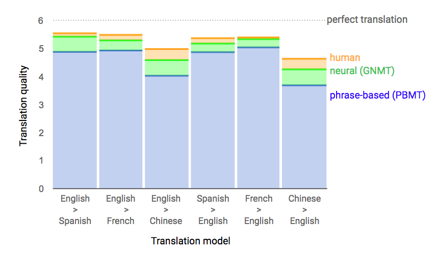
Data from side-by-side evaluations, where human raters compare the quality of translations for a given source sentence. Scores range from 0 to 6, with 0 meaning “completely nonsense translation”, and 6 meaning “perfect translation."
The following visualization shows the progression of GNMT as it translates a Chinese sentence to English. First, the network encodes the Chinese words as a list of vectors, where each vector represents the meaning of all words read so far (“Encoder”). Once the entire sentence is read, the decoder begins, generating the English sentence one word at a time (“Decoder”). To generate the translated word at each step, the decoder pays attention to a weighted distribution over the encoded Chinese vectors most relevant to generate the English word (“Attention”; the blue link transparency represents how much the decoder pays attention to an encoded word).
Using human-rated side-by-side comparison as a metric, the GNMT system produces translations that are vastly improved compared to the previous phrase-based production system. GNMT reduces translation errors by more than 55%-85% on several major language pairs measured on sampled sentences from Wikipedia and news websites with the help of bilingual human raters.
An example of a translation produced by our system for an input sentence sampled from a news site. Go here for more examples of translations for input sentences sampled randomly from news sites and books.
In addition to releasing this research paper today, we are announcing the launch of GNMT in production on a notoriously difficult language pair: Chinese to English. The Google Translate mobile and web apps are now using GNMT for 100% of machine translations from Chinese to English—about 18 million translations per day. The production deployment of GNMT was made possible by use of our publicly available machine learning toolkit TensorFlow and our Tensor Processing Units (TPUs), which provide sufficient computational power to deploy these powerful GNMT models while meeting the stringent latency requirements of the Google Translate product. Translating from Chinese to English is one of the more than 10,000 language pairs supported by Google Translate, and we will be working to roll out GNMT to many more of these over the coming months.
Machine translation is by no means solved. GNMT can still make significant errors that a human translator would never make, like dropping words and mistranslating proper names or rare terms, and translating sentences in isolation rather than considering the context of the paragraph or page. There is still a lot of work we can do to serve our users better. However, GNMT represents a significant milestone. We would like to celebrate it with the many researchers and engineers—both within Google and the wider community—who have contributed to this direction of research in the past few years.
References: [1] Google’s Neural Machine Translation System: Bridging the Gap between Human and Machine Translation, Yonghui Wu, Mike Schuster, Zhifeng Chen, Quoc V. Le, Mohammad Norouzi, Wolfgang Macherey, Maxim Krikun, Yuan Cao, Qin Gao, Klaus Macherey, Jeff Klingner, Apurva Shah, Melvin Johnson, Xiaobing Liu, Łukasz Kaiser, Stephan Gouws, Yoshikiyo Kato, Taku Kudo, Hideto Kazawa, Keith Stevens, George Kurian, Nishant Patil, Wei Wang, Cliff Young, Jason Smith, Jason Riesa, Alex Rudnick, Oriol Vinyals, Greg Corrado, Macduff Hughes, Jeffrey Dean. Technical Report, 2016. [2] Sequence to Sequence Learning with Neural Networks, Ilya Sutskever, Oriol Vinyals, Quoc V. Le. Advances in Neural Information Processing Systems, 2014. [3] Addressing the rare word problem in neural machine translation, Minh-Thang Luong, Ilya Sutskever, Quoc V. Le, Oriol Vinyals, and Wojciech Zaremba. Proceedings of the 53th Annual Meeting of the Association for Computational Linguistics, 2015. [4] Neural Machine Translation by Jointly Learning to Align and Translate, Dzmitry Bahdanau, Kyunghyun Cho, Yoshua Bengio. International Conference on Learning Representations, 2015. [5] Japanese and Korean voice search, Mike Schuster, and Kaisuke Nakajima. IEEE International Conference on Acoustics, Speech and Signal Processing, 2012. [6] Neural Machine Translation of Rare Words with Subword Units, Rico Sennrich, Barry Haddow, Alexandra Birch. Proceedings of the 54th Annual Meeting of the Association for Computational Linguistics, 2016.
Our 2014 system used the Inception V1 image classification model to initialize the image encoder, which produces the encodings that are useful for recognizing different objects in the images. This was the best image model available at the time, achieving 89.6% top-5 accuracy on the benchmark ImageNet 2012 image classification task. We replaced this in 2015 with the newer Inception V2 image classification model, which achieves 91.8% accuracy on the same task. The improved vision component gave our captioning system an accuracy boost of 2 points in the BLEU-4 metric (which is commonly used in machine translation to evaluate the quality of generated sentences) and was an important factor of its success in the captioning challenge.
Today’s code release initializes the image encoder using the Inception V3 model, which achieves 93.9% accuracy on the ImageNet classification task. Initializing the image encoder with a better vision model gives the image captioning system a better ability to recognize different objects in the images, allowing it to generate more detailed and accurate descriptions. This gives an additional 2 points of improvement in the BLEU-4 metric over the system used in the captioning challenge.
Another key improvement to the vision component comes from fine-tuning the image model. This step addresses the problem that the image encoder is initialized by a model trained to classify objects in images, whereas the goal of the captioning system is to describe the objects in images using the encodings produced by the image model. For example, an image classification model will tell you that a dog, grass and a frisbee are in the image, but a natural description should also tell you the color of the grass and how the dog relates to the frisbee.
In the fine-tuning phase, the captioning system is improved by jointly training its vision and language components on human generated captions. This allows the captioning system to transfer information from the image that is specifically useful for generating descriptive captions, but which was not necessary for classifying objects. In particular, after fine-tuning it becomes better at correctly describing the colors of objects. Importantly, the fine-tuning phase must occur after the language component has already learned to generate captions - otherwise, the noisiness of the randomly initialized language component causes irreversible corruption to the vision component. For more details, read the full paper here.
Left: the better image model allows the captioning model to generate more detailed and accurate descriptions. Right: after fine-tuning the image model, the image captioning system is more likely to describe the colors of objects correctly.
Until recently our image captioning system was implemented in the DistBelief software framework. The TensorFlow implementation released today achieves the same level of accuracy with significantly faster performance: time per training step is just 0.7 seconds in TensorFlow compared to 3 seconds in DistBelief on an Nvidia K20 GPU, meaning that total training time is just 25% of the time previously required.
A natural question is whether our captioning system can generate novel descriptions of previously unseen contexts and interactions. The system is trained by showing it hundreds of thousands of images that were captioned manually by humans, and it often re-uses human captions when presented with scenes similar to what it’s seen before.
When the model is presented with scenes similar to what it’s seen before, it will often re-use human generated captions.
So does it really understand the objects and their interactions in each image? Or does it always regurgitate descriptions from the training data? Excitingly, our model does indeed develop the ability to generate accurate new captions when presented with completely new scenes, indicating a deeper understanding of the objects and context in the images. Moreover, it learns how to express that knowledge in natural-sounding English phrases despite receiving no additional language training other than reading the human captions.
Our model generates a completely new caption using concepts learned from similar scenes in the training set.
We hope that sharing this model in TensorFlow will help push forward image captioning research and applications, and will also allow interested people to learn and have fun. To get started training your own image captioning system, and for more details on the neural network architecture, navigate to the model’s home-page here. While our system uses the Inception V3 image classification model, you could even try training our system with the recently released Inception-ResNet-v2 model to see if it can do even better!
Posted by Alex Alemi, Software Engineer Earlier this week, we announced the latest release of the TF-Slim library for TensorFlow, a lightweight package for defining, training and evaluating models, as well as checkpoints and model definitions for several competitive networks in the field of image classification.
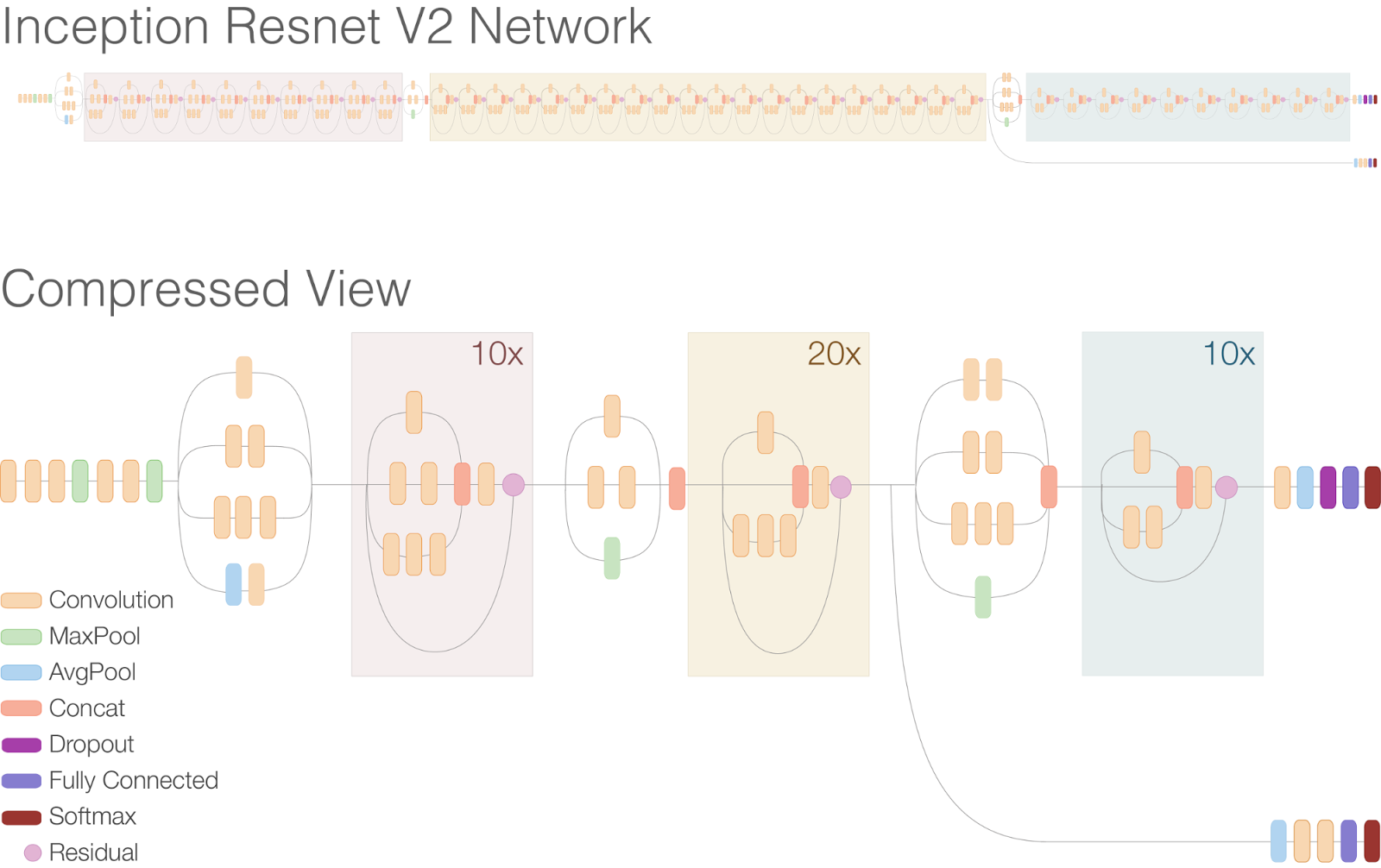
Residual connections allow shortcuts in the model and have allowed researchers to successfully train even deeper neural networks, which have lead to even better performance. This has also enabled significant simplification of the Inception blocks. Just compare the model architectures in the figures below:
Schematic diagram of Inception V3
Schematic diagram of Inception-ResNet-v2
At the top of the second Inception-ResNet-v2 figure, you'll see the full network expanded. Notice that this network is considerably deeper than the previous Inception V3. Below in the main figure is an easier to read version of the same network where the repeated residual blocks have been compressed. Here, notice that the inception blocks have been simplified, containing fewer parallel towers than the previous Inception V3.
The Inception-ResNet-v2 architecture is more accurate than previous state of the art models, as shown in the table below, which reports the Top-1 and Top-5 validation accuracies on the ILSVRC 2012 image classification benchmark based on a single crop of the image. Furthermore, this new model only requires roughly twice the memory and computation compared to Inception V3.
As an example, while both Inception V3 and Inception-ResNet-v2 models excel at identifying individual dog breeds, the new model does noticeably better. For instance, whereas the old model mistakenly reported Alaskan Malamute for the picture on the right, the new Inception-ResNet-v2 model correctly identifies the dog breeds in both images.
We are excited to see what the community does with this improved model, following along as people adapt it and compare its performance on various tasks. Want to get started? See the accompanying instructions on how to train, evaluate or fine-tune a network.
As always, releasing the code was a team effort. Specific thanks are due to:
Model Architecture - Christian Szegedy, Sergey Ioffe, Vincent Vanhoucke, Alex Alemi
Systems Infrastructure - Jon Shlens, Benoit Steiner, Mark Sandler, and David Andersen
TensorFlow-Slim - Sergio Guadarrama and Nathan Silberman
Model Visualization - Fernanda Viégas and James Wexler
Posted by Nathan Silberman and Sergio Guadarrama, Google Research
Earlier this year, we released a TensorFlow implementation of a state-of-the-art image classification model known as Inception-V3. This code allowed users to train the model on the ImageNet classification dataset via synchronized gradient descent, using either a single local machine or a cluster of machines. The Inception-V3 model was built on an experimental TensorFlow library called TF-Slim, a lightweight package for defining, training and evaluating models in TensorFlow. The TF-Slim library provides common abstractions which enable users to define models quickly and concisely, while keeping the model architecture transparent and its hyperparameters explicit.
Since that release, TF-Slim has grown substantially, with many types of layers, loss functions, and evaluation metrics added, along with handy routines for training and evaluating models. These routines take care of all the details you need to worry about when working at scale, such as reading data in parallel, deploying models on multiple machines, and more. Additionally, we have created the TF-Slim Image Models library, which provides definitions and training scripts for many widely used image classification models, using standard datasets. TF-Slim and its components are already widely used within Google, and many of these improvements have already been integrated into tf.contrib.slim.
Today, we are proud to share the latest release of TF-Slim with the TF community. Some highlights of this release include:
Support for more loss functions and evaluation metrics (e.g., mAP, IoU).
A deployment library to make it easier to perform synchronous or asynchronous training using multiple GPUs/CPUs, on the same machine or on multiple machines.
Code to define and train many widely used image classification models (e.g., Inception[1][2][3], VGG[4], AlexNet[5], ResNet[6]).
Pre-trained model weights for the above image classification models. These models have been trained on the ImageNet classification dataset, but can be used for many other computer vision tasks. As a simple example, we provide code to fine-tune these classifiers to a new set of output labels.
Want to get started using TF-Slim? See the README for details. Interested in working with image classification models? See these instructions or this Jupyter notebook.
The release of the TF-Slim library and the pre-trained model zoo has been the result of widespread collaboration within Google Research. In particular we want to highlight the vital contributions of the following researchers:
TF-Slim: Sergio Guadarrama, Nathan Silberman.
Model Definitions and Checkpoints: Christian Szegedy, Sergey Ioffe, Vincent Vanhoucke, Jon Shlens, Zbigniew Wojna, Vivek Rathod, George Papandreou, Alex Alemi
Systems Infrastructure: Jon Shlens, Matthieu Devin, Martin Wicke


