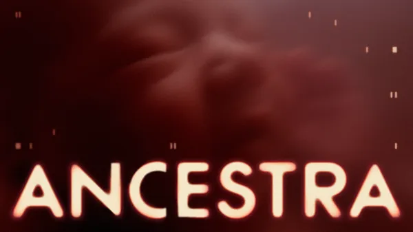We partnered with Darren Aronofsky, Eliza McNitt and a team of more than 200 to make ANCESTRA.

We partnered with Darren Aronofsky, Eliza McNitt and a team of more than 200 to make ANCESTRA.

We partnered with Darren Aronofsky, Eliza McNitt and a team of more than 200 to make ANCESTRA.

We partnered with Darren Aronofsky, Eliza McNitt and a team of more than 200 to make ANCESTRA.

We partnered with Darren Aronofsky, Eliza McNitt and a team of more than 200 to make ANCESTRA.

We partnered with Darren Aronofsky, Eliza McNitt and a team of more than 200 to make ANCESTRA.

We partnered with Darren Aronofsky, Eliza McNitt and a team of more than 200 to make ANCESTRA.

We partnered with Darren Aronofsky, Eliza McNitt and a team of more than 200 to make ANCESTRA.

We partnered with Darren Aronofsky, Eliza McNitt and a team of more than 200 to make ANCESTRA.

We partnered with Darren Aronofsky, Eliza McNitt and a team of more than 200 to make ANCESTRA.