By Michael D. Moffitt, Core Enterprise Machine Learning
Tag Archives: optimization
Robust Routing Using Electrical Flows
In the world of networks, there are models that can explain observations across a diverse collection of applications. These include simple tasks such as computing the shortest path, which has obvious applications to routing networks but also in biology, where the slime mold Physarum is able to find shortest paths in mazes. Another example is Braess’s paradox — the observation that adding resources to a network can have an effect opposite to the one expected — which manifests not only in road networks but also in mechanical and electrical systems, which can also be modeled as networks. For instance, constructing a new road can increase traffic congestion or adding a new link in an electrical circuit can increase voltage. Such connections between electrical circuits and other types of networks have been exploited for various tasks, such as partitioning networks, and routing flows.
In “Robust Routing Using Electrical Flows”, which won the Best Paper Award at SIGSPATIAL 2021, we present another interesting application of electrical flows in the context of road network routing. Specifically, we utilize ideas from electrical flows for the problem of constructing multiple alternate routes between a given source and destination. Alternate routes are important for many use cases, including finding routes that best match user preferences and for robust routing, e.g., routing that guarantees finding a good path in the presence of traffic jams. Along the way, we also describe how to quickly model electrical flows on road networks.
Existing Approaches to Alternate Routing
Computing alternate routes on road networks is a relatively new area of research and most techniques rely on one of two main templates: the penalty method and the plateau method. In the former, alternate routes are iteratively computed by running a shortest path algorithm and then, in subsequent runs, adding a penalty to those segments already included in the shortest paths that have been computed, to encourage further exploration. In the latter, two shortest path trees are built simultaneously, one starting from the origin and one from the destination, which are used to identify sequences of road segments that are common to both trees. Each such common sequence (which are expected to be important arterial streets for example) is then treated as a visit point on the way from the origin to the destination, thus potentially producing an alternate route. The penalty method is known to produce results of high quality (i.e., average travel time, diversity and robustness of the returned set of alternate routes) but is very slow in practice, whereas the plateau method is much faster but results in lower quality solutions.
An Alternate to Alternate Routing: Electrical Flows
Our approach is different and assumes that a routing problem on a road network is in many ways analogous to the flow of electrical current through a resistor network. Though the electrical current travels through many different paths, it is weaker along paths of higher resistance and stronger on low resistance ones, all else being equal.
We view the road network as a graph, where intersections are nodes and roads are edges. Our method then models the graph as an electrical circuit by replacing the edges with resistors, whose resistances equal the road traversal time, and then connecting a battery to the origin and destination, which results in electrical current between those two points. In this analogy, the resistance models how time-consuming it is to traverse a segment. In this sense, long and congested segments have high resistances. Intuitively speaking, the flow of electrical current will be spread around the entire network but concentrated on the routes that have lower resistance, which correspond to faster routes. By identifying the primary routes taken by the current, we can construct a viable set of alternates from origin to destination.
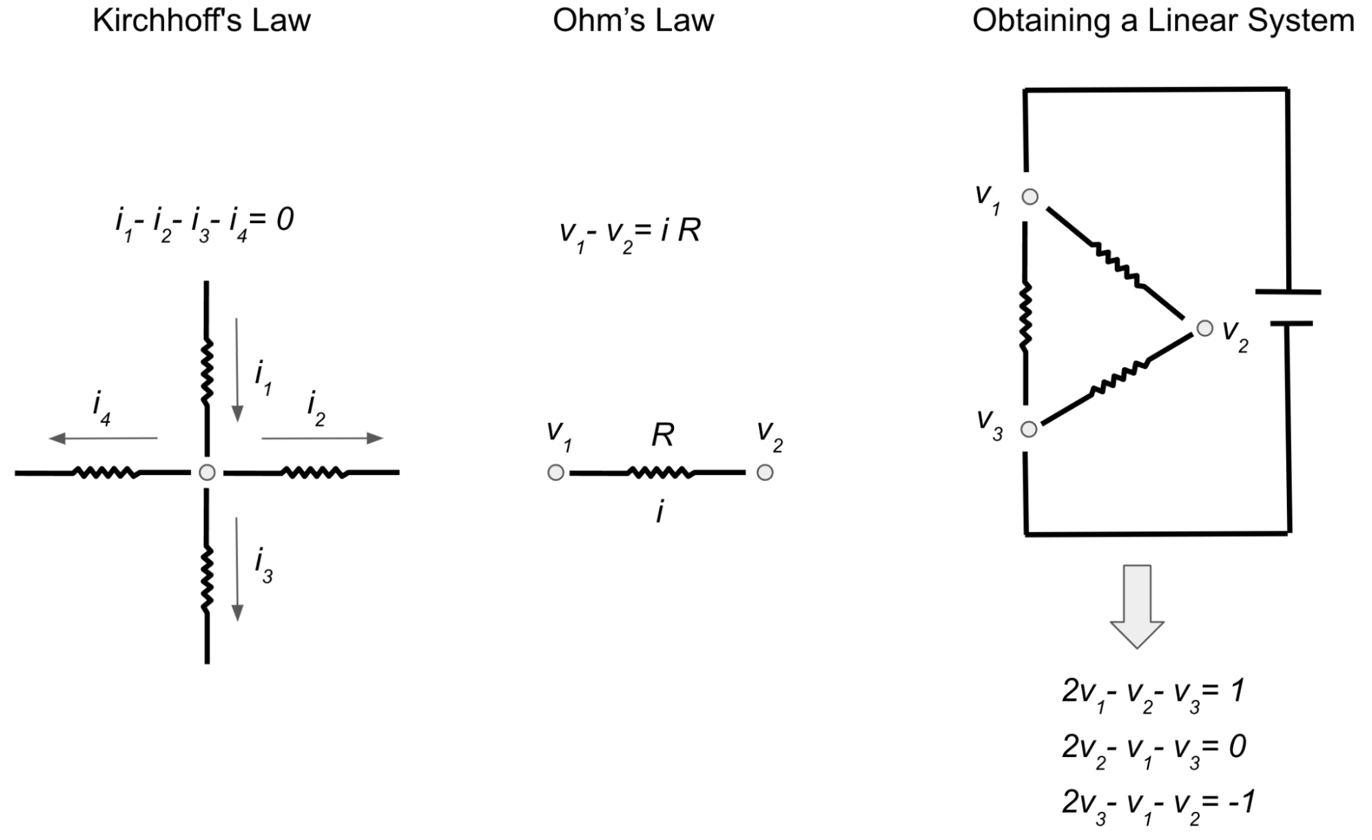
In order to compute the electrical flow, we use Kirchhoff’s and Ohm’s laws, which say respectively: 1) the algebraic sum of currents at each junction is equal to zero, meaning that the traffic that enters any intersection also exits it (for instance if three cars enter an intersection from one street and another car enters the same intersection from another street, a total of four cars need to exit the intersection); and 2) the current is directly proportional to the voltage difference between endpoints. If we write down the resulting equations, we end up with a linear system with n equations over n variables, which correspond to the potentials (i.e, the voltage) at each intersection. While voltage has no direct analogy to road networks, it can be used to help compute the flow of electrical current and thus find alternate routes as described above.
So the computation boils down to computing values for the variables of this linear system involving a very special matrix called Laplacian matrix. Such matrices have many useful properties, e.g., they are symmetric and sparse — the number of off-diagonal non-zero entries is equal to twice the number of edges. Even though there are many existing near-linear time solvers for such systems of linear equations, they are still too slow for the purposes of quickly responding to routing requests with low latency. Thus we devised a new algorithm that solves these linear systems much faster for the special case of road networks1.
Fast Electrical Flow Computation
The first key part of this new algorithm involves Gaussian elimination, which is possibly the most well-known method for solving linear systems. When performed on a Laplacian matrix corresponding to some resistor network, it corresponds to the Y-Δ transformation, which reduces the number of nodes, while preserving the voltages. The only downside is that the number of edges may increase, which would make the linear system even slower to solve. For example, if a node with 10 connections is eliminated using the Y-Δ transformation, the system would end up with 35 new connections!
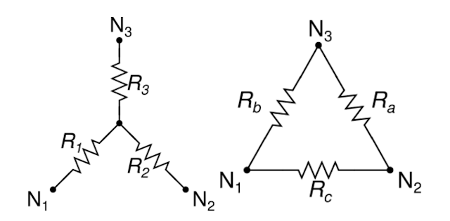 |
| The Y-Δ transformation allows us to remove the middle junction and replace it with three connections (Ra, Rb and Rc) between N1, N2 and N3. (Image from Wikipedia) |
However if one can identify parts of the network that are connected to the rest through very few nodes (lets call these connections bottlenecks), and perform elimination on everything else while leaving the bottleneck nodes, the new edges formed at the end will only be between bottleneck nodes. Provided that the number of bottleneck nodes is much smaller than the number of nodes eliminated with Y-Δ — which is true in the case of road networks since bottleneck nodes, such as bridges and tunnels, are much less common than regular intersections — this will result in a large net decrease (e.g., ~100x) in terms of graph size. Fortunately, identifying such bottlenecks in road networks can be done easily by partitioning such a network. By applying Y-Δ transformation to all nodes except the bottlenecks2, the result is a much smaller graph for which the voltages can be solved faster.
But what about computing the currents on the rest of the network, which is not made up of bottleneck nodes? A useful property about electrical flows is that once the voltages on bottleneck nodes are known, one can easily compute the electrical flow for the rest of the network. The electrical flow inside a part of the network only depends on the voltage of bottleneck nodes that separate that part from the rest of the network. In fact, it’s possible to precompute a small matrix so that one can recover the electrical flow by a single matrix-vector multiplication, which is a very fast operation that can be run in parallel.
Once we obtain a solution that gives the electrical flow in our model network, we can observe the routes that carry the highest amount of electrical flow and output those as alternate routes for the road network.
Results
Here are some results depicting the alternates computed by the above algorithm.
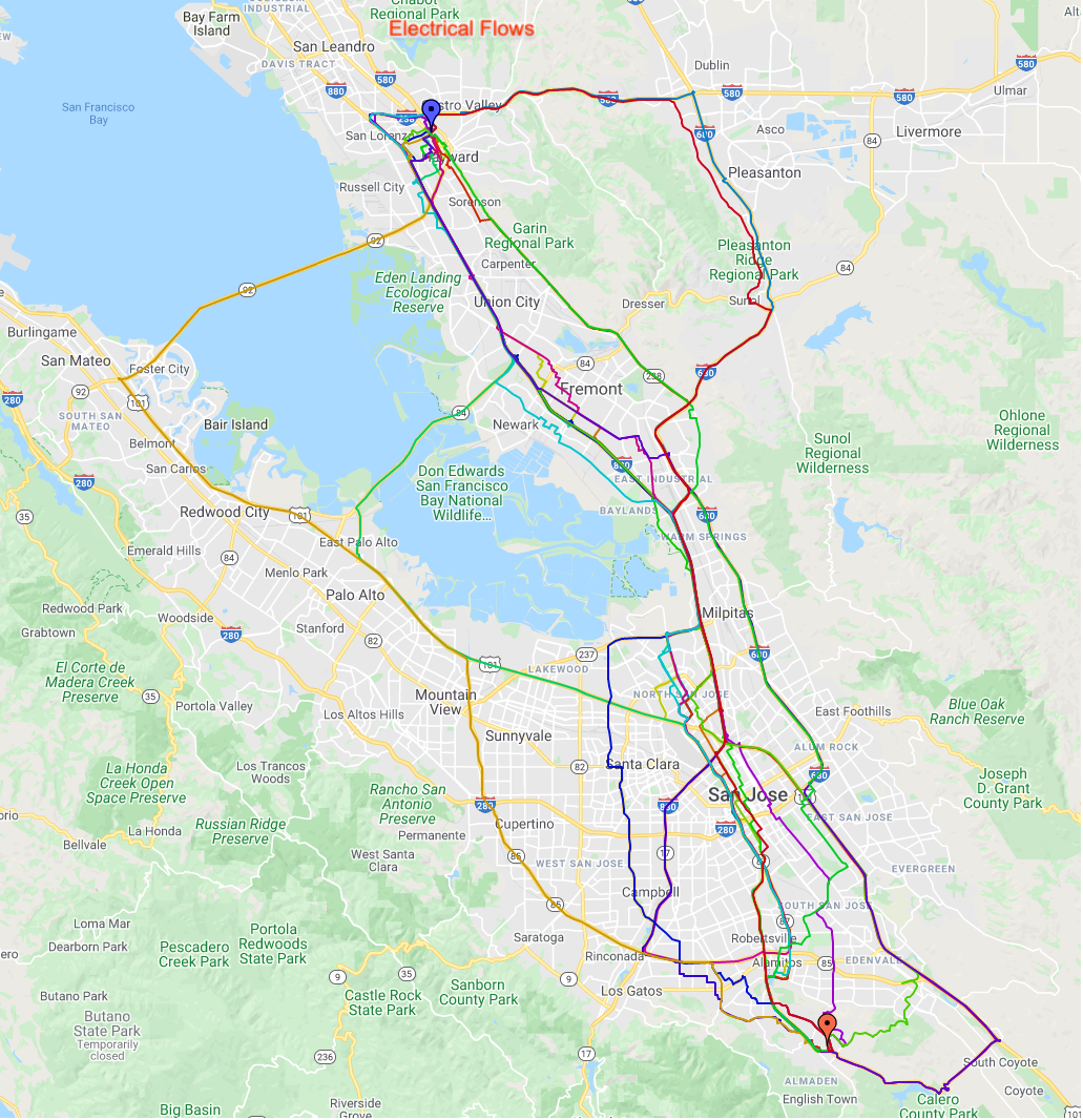 |
| Different alternates found for the Bay Area. Different colors correspond to different routes. |
Conclusion
In this post we describe a novel approach for computing alternate routes in road networks. Our approach is fundamentally different from the main techniques applied in decades of research in the area and provides high quality alternate routes in road networks by studying the problem through the lens of electrical circuits. This is an approach that can prove very useful in practical systems and we hope inspires more research in the area of alternate route computation and related problems. Interested readers can find a more detailed discussion of this work in our SIGSPATIAL 2021 talk recording.
Acknowledgements
We thank our collaborators Lisa Fawcett, Sreenivas Gollapudi, Ravi Kumar, Andrew Tomkins and Ameya Velingker from Google Research.
1Our techniques work for any network that can be broken down to smaller components with the removal of a few nodes. ↩
2 Performing Y-Δ transformation one-by-one for each node will be too slow. Instead we eliminate whole groups of nodes by taking advantage of the algebraic properties of Y-Δ transformation. ↩
Source: Google AI Blog
Upcoming changes to Simulations in the Google Ads API and Bid Landscapes in the AdWords API
We are changing the way ad group simulations with SimulationModificationMethod = DEFAULT are calculated in the Google Ads API and the AdWords API.
What’s changing?
For an ad group with keyword bid overrides, we provide estimated traffic for different values of the ad group’s default bid. Currently, all keywords with bid overrides are excluded from this estimate. This results in a lower-than-expected traffic estimate.
Starting the week of January 17, 2022, we will modify our estimation to include both keywords using the default bid and keywords with bid overrides when calculating ad group simulations. We will further assume that only the ad group default bid would change in the simulation, and all keyword bid overrides will remain the same. This may affect the simulations returned by the GetAdGroupSimulation method of the AdGroupSimulationService service in the Google Ads API and the getAdGroupBidLandscape and queryAdGroupBidLandscape methods of the DataService service in the AdWords API.
What should you do?
If you use this feature, we recommend that you ensure that your code continues to work with the modified results returned by these methods.
If you have any questions, please contact us via the Google Ads API forum.
Reminder: Share your feedback about the Google Ads (AdWords) API. Take the 2021 AdWords API and Google Ads API Annual Survey.
Source: Google Ads Developer Blog
JuMP: A modeling language for mathematical optimization
JuMP was created—in the classical open source fashion—to scratch an itch. As graduate students, we wanted a software package that would enable us to write down and solve optimization problems, especially constrained optimization problems like linear programming and integer programming problems. We wanted it to be not only easy, but also fast and powerful. At the time, one was faced with trade-offs between ease-of-use, speed, and flexibility. For example, optimization libraries in Python were user-friendly but introduced noticeable performance bottlenecks. Commercial software such as AMPL was efficient but hard to extend. Low-level interfaces in C or C++ introduced complexities that were distracting for teaching and academic research. We weren’t satisfied with these trade-offs, and began experimenting with a new programming language called Julia that promised to provide the best of both worlds.
Our early experiments showed that Julia was indeed capable of impressive performance. While similar libraries based on Python could be slower to construct the data structure describing the optimization problem than to solve it, our prototype of JuMP was competitive with state-of-the-art commercial libraries. This gave us confidence that JuMP could be useful for the community, and we made the initial public release in October 2013.
Since then, it’s been a real ride! The first JuMP developers workshop in 2017 attracted thirteen speakers from four continents; this year’s workshop featured 32 virtual talks. Of the 800+ citations to the award-winning paper, we were surprised to discover that that about 75% of them were from outside the fields of operations research or optimization itself; about 20% are in energy and power systems, another 20% are in control and engineering, and the remaining citations are spread across scientific applications, computer science, machine learning, and other fields. These figures speak to the role of optimization as a fundamental technology that can be applied almost anywhere. One example application using JuMP of which I’m perhaps most proud is a study by Sepulveda et al. on cost-effective ways to decarbonize the power grid. This study is cited both by Bill Gates in his new book, “How to Avoid a Climate Disaster,” and by Google’s methodologies and metrics framework for its goal of operating data centers and campuses entirely on carbon-free energy by 2030.
As JuMP’s core development team grew beyond MIT and its original creators graduated, it was important for JuMP to find a new home for its long-term sustainability. We were lucky to find NumFOCUS, a nonprofit organization supporting open source scientific software (of which Google is a corporate sponsor). As a Google employee, I have continued contributing code for JuMP, traveling to workshops, and serving in leadership roles thanks in no small part to Google’s generous open source policies and support from my team and management chain. Last year, I was granted the honorific of Benevolent Dictator for Life (BDFL). I plan to use this power judiciously and rarely, relying instead on JuMP’s strong culture of consensus-driven development.
As for the future, JuMP’s 1.0 release is near on the horizon, and I look forward to whatever comes next!
By Miles Lubin, Algorithms & Optimization Team, Google Research
Source: Google Open Source Blog
Sunsetting the KEYWORD_MATCH_TYPE recommendation type
KEYWORD_MATCH_TYPE will be removed and no new recommendations of this type will be generated anymore.What's changing?
The
KEYWORD_MATCH_TYPE recommendations will no longer be returned by search for all versions of the Google Ads API and Google Ads scripts.All requests sent to apply or dismiss
KEYWORD_MATCH_TYPE recommendations will fail with RequestError.RESOURCE_NOT_FOUND errors for all versions of the Google Ads API.What do you need to do?
Before July 21, 2021, ensure that the changes described above will not lead to any issues in your code or application.
Then, as soon as you can, remove any references of the field
Recommendation.keyword_match_type_recommendation and the type KeywordMatchTypeRecommendation in your code. They will be deprecated and removed in future versions.If you have any questions or need additional help, contact us through the forum or at [email protected].
Source: Google Ads Developer Blog
Improving Sparse Training with RigL
Modern deep neural network architectures are often highly redundant [1, 2, 3], making it possible to remove a significant fraction of connections without harming performance. The sparse neural networks that result have been shown to be more parameter and compute efficient compared to dense networks, and, in many cases, can significantly decrease wall clock inference times.
By far the most popular method for training sparse neural networks is pruning, (dense-to-sparse training) which usually requires first training a dense model, and then “sparsifying” it by cutting out the connections with negligible weights. However, this process has two limitations.
- The size of the largest trainable sparse model is limited by that of the largest trainable dense model. Even if sparse models are more parameter efficient, one cannot use pruning to train models that are larger and more accurate than the largest possible dense models.
- Pruning is inefficient, meaning that large amounts of computation must be performed for parameters that are zero valued or that will be zero during inference. Additionally, it remains unknown if the performance of the current best pruning algorithms are an upper bound on the quality of sparse models.
In “Rigging the Lottery: Making All Tickets Winners”, presented at ICML 2020, we introduce RigL, an algorithm for training sparse neural networks that uses a fixed parameter count and computational cost throughout training, without sacrificing accuracy relative to existing dense-to-sparse training methods. The algorithm identifies which neurons should be active during training, which helps the optimization process to utilize the most relevant connections and results in better sparse solutions. An example of this is shown below, where, during the training of a multilayer perceptron (MLP) network on MNIST, our sparse network trained with RigL learns to focus on the center of the images, discarding the uninformative pixels from the edges. A Tensorflow implementation of our method along with three other baselines (SET, SNFS, SNIP) can be found at github.com/google-research/rigl.
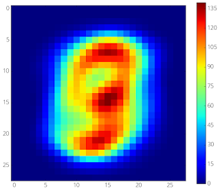 |  |
| Left: Average MNIST image. Right: Evolution of the connectivity of the input throughout the training of a 98% sparse, 2-layer MLP on MNIST. Training starts from a random sparse mask, where each input pixel has roughly six outgoing connections. Connections that originate from the edges do not exhibit meaningful gradients and are therefore replaced by more informative connections that originate from the center pixels. |
RigL Overview
The RigL method starts with a network initialized with a random sparse topology. At regularly spaced intervals we remove a fraction of the connections with the smallest weight magnitudes. Such a strategy has been shown to have very little effect on the loss. RigL then activates new connections using instantaneous gradient information, i.e., without using past gradient information. After updating the connectivity, training continues with the updated network until the next scheduled update. Next, the system activates connections with large gradients, since these connections are expected to decrease the loss most quickly.
Evaluating Performance
By changing the connectivity of the neurons dynamically during training, RigL helps optimize to find better solutions. To demonstrate this, we restart training from a bad solution that exhibits poor accuracy and show that RigL's mask updates help the optimization achieve better loss compared to static training, in which connectivity of the sparse network remains the same.
 |
| Training loss of RigL and Static methods starting from the same static sparse solution, shown together with their final test accuracies. |
The figure below summarizes the performance of various methods on training an 80% sparse ResNet-50 architecture. We compare RigL with two recent sparse training methods, SET and SNFS and three baseline training methods: Static, Small-Dense and Pruning. Two of these methods (SNFS and Pruning) require dense resources as they need to either train a large network or store the gradients of it. Overall, we observe that the performance of all methods improves with additional training time; thus, for each method we run extended training with up to 5x the training steps of the original 100 epochs.
As noted in a number of studies [4, 5, 6, 7], training a network with fixed sparsity from scratch (Static) leads to inferior performance compared to solutions found by pruning. Training a small, dense network (Small-Dense) with the same number of parameters gets better results than Static, but fails to match the performance of dynamic sparse models. Similarly, SET improves the performance over Small-Dense, but saturates at around 75% accuracy, revealing the limits of growing new connections randomly. Methods that use gradient information to grow new connections (RigL and SNFS) obtain higher accuracy in general, but RigL achieves the highest accuracy, while also consistently requiring fewer FLOPs (and memory footprint) than the other methods.
Observing the trend between extended training and performance, we compare the results using longer training runs. Within the interval considered (i.e., 1x-100x) RigL's performance constantly improves with additional training. RigL achieves state of art performance of 68.07% Top-1 accuracy at training with a 99% sparse ResNet-50 architecture. Similarly extended training of a 90% sparse MobileNet-v1 architecture with RigL achieves 70.55% Top-1 accuracy. Obtaining the same results with fewer training iterations is an exciting future research direction.
 |  |
| Effect of training time on RigL accuracy at training 99% sparse ResNet-50 (left) and 90% sparse MobileNets-v1 (right) architectures. |
Other experiments include image classification on CIFAR-10 datasets and character-based language modelling using RNNs with the WikiText-103 dataset and can be found in the full paper.
Future Work
RigL is useful in three different scenarios:
- Improving the accuracy of sparse models intended for deployment.
- Improving the accuracy of large sparse models that can only be trained for a limited number of iterations.
- Combining with sparse primitives to enable training of extremely large sparse models which otherwise would not be possible.
AcknowledgementsWe would like to thank Eleni Triantafillou, Hugo Larochelle, Bart van Merrienboer, Fabian Pedregosa, Joan Puigcerver, Danny Tarlow, Nicolas Le Roux, Karen Simonyan for giving feedback on the preprint of the paper; Namhoon Lee for helping us verify and debug our SNIP implementation; Chris Jones for helping us discover and solve the distributed training bug; and Tom Small for creating the visualization of the algorithm.
Source: Google AI Blog
Speeding Up Neural Network Training with Data Echoing
Over the past decade, dramatic increases in neural network training speed have made it possible to apply deep learning techniques to many important problems. In the twilight of Moore's law, as improvements in general purpose processors plateau, the machine learning community has increasingly turned to specialized hardware to produce additional speedups. For example, GPUs and TPUs optimize for highly parallelizable matrix operations, which are core components of neural network training algorithms. These accelerators, at a high level, can speed up training in two ways. First, they can process more training examples in parallel, and second, they can process each training example faster. We know there are limits to the speedups from processing more training examples in parallel, but will building ever faster accelerators continue to speed up training?
Unfortunately, not all operations in the training pipeline run on accelerators, so one cannot simply rely on faster accelerators to continue driving training speedups. For example, earlier stages in the training pipeline like disk I/O and data preprocessing involve operations that do not benefit from GPUs and TPUs. As accelerator improvements outpace improvements in CPUs and disks, these earlier stages will increasingly become a bottleneck, wasting accelerator capacity and limiting training speed.
 |
| An example training pipeline representative of many large-scale computer vision programs. The stages that come before applying the mini-batch stochastic gradient descent (SGD) update generally do not benefit from specialized hardware accelerators. |
In “Faster Neural Network Training with Data Echoing”, we propose a simple technique that reuses (or “echoes”) intermediate outputs from earlier pipeline stages to reclaim idle accelerator capacity. Rather than waiting for more data to become available, we simply utilize data that is already available to keep the accelerators busy.
 |
| Left: Without data echoing, downstream computational capacity is idle 50% of the time. Right: Data echoing with echoing factor 2 reclaims downstream computational capacity. |
Imagine a situation where reading and preprocessing a batch of training data takes twice as long as performing a single optimization step on that batch. In this case, after the first optimization step on the preprocessed batch, we can reuse the batch and perform a second step before the next batch is ready. In the best case scenario, where repeated data is as useful as fresh data, we would see a twofold speedup in training. In reality, data echoing provides a slightly smaller speedup because repeated data is not as useful as fresh data – but it can still provide a significant speedup compared to leaving the accelerator idle.
There are typically several ways to implement data echoing in a given neural network training pipeline. The technique we propose involves duplicating data into a shuffle buffer somewhere in the training pipeline, but we are free to insert this buffer anywhere after whichever stage produces a bottleneck in the given pipeline. When we insert the buffer before batching, we call our technique example echoing, whereas, when we insert it after batching, we call our technique batch echoing. Example echoing shuffles data at the example level, while batch echoing shuffles the sequence of duplicate batches. We can also insert the buffer before data augmentation, such that each copy of repeated data is slightly different (and therefore closer to a fresh example). Of the different versions of data echoing that place the shuffle buffer between different stages, the version that provides the greatest speedup depends on the specific training pipeline.
Data Echoing Across Workloads
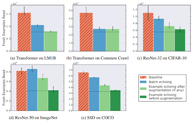
So how useful is reusing data? We tried data echoing on five neural network training pipelines spanning 3 different tasks – image classification, language modeling, and object detection – and measured the number of fresh examples needed to reach a particular performance target. We chose targets to match the best result reliably achieved by the baseline during hyperparameter tuning. We found that data echoing allowed us to reach the target performance with fewer fresh examples, demonstrating that reusing data is useful for reducing disk I/O across a variety of tasks. In some cases, repeated data is nearly as useful as fresh data: in the figure below, example echoing before augmentation reduces the number of fresh examples required almost by the repetition factor.
Data echoing can speed up training whenever computation upstream from accelerators dominates training time. We measured the training speedup achieved in a training pipeline bottlenecked by input latency due to streaming training data from cloud storage, which is realistic for many of today’s large-scale production workloads or anyone streaming training data over a network from a remote storage system. We trained a ResNet-50 model on the ImageNet dataset and found that data echoing provides a significant training speedup, in this case, more than 3 times faster when using data echoing.
Although one might be concerned that reusing data would harm the model’s final performance, we found that data echoing did not degrade the quality of the final model for any of the workloads we tested.
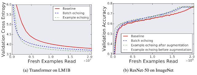 |
| Comparing the individual trials that achieved the best out-of-sample performance during training for both with and without data echoing shows that reusing data does not harm final model quality. Here validation cross entropy is equivalent to log perplexity. |
Acknowledgements
The Data Echoing project was conducted by Dami Choi, Alexandre Passos, Christopher J. Shallue, and George E. Dahl while Dami Choi was a Google AI Resident. We would also like to thank Roy Frostig, Luke Metz, Yiding Jiang, and Ting Chen for helpful discussions.
Source: Google AI Blog
Bi-Tempered Logistic Loss for Training Neural Nets with Noisy Data
The quality of models produced by machine learning (ML) algorithms directly depends on the quality of the training data, but real world datasets typically contain some amount of noise that introduces challenges for ML models. Noise in the dataset can take several forms from corrupted examples (e.g., lens flare in an image of a cat) to mislabelled examples from when the data was collected (e.g., an image of cat mislabelled as a flerken).
The ability of an ML model to deal with noisy training data depends in great part on the loss function used in the training process. For classification tasks, the standard loss function used for training is the logistic loss. However, this particular loss function falls short when handling noisy training examples due to two unfortunate properties:
- Outliers far away can dominate the overall loss: The logistic loss function is sensitive to outliers. This is because the loss function value grows without bound as the mislabelled examples (outliers) are far away from the decision boundary. Thus, a single bad example that is located far away from the decision boundary can penalize the training process to the extent that the final trained model learns to compensate for it by stretching the decision boundary and potentially sacrificing the remaining good examples. This “large-margin” noise issue is illustrated in the left panel of the figure below.
- Mislabeled examples nearby can stretch the decision boundary: The output of the neural network is a vector of activation values, which reflects the margin between the example and the decision boundary for each class. The softmax transfer function is used to convert the activation values into probabilities that an example will belong to each class. As the tail of this transfer function for the logistic loss decays exponentially fast, the training process will tend to stretch the boundary closer to a mislabeled example in order to compensate for its small margin. Consequently, the generalization performance of the network will immediately deteriorate, even with a low level of label noise (right panel below).
 |  |
| We visualize the decision surface of a 2-layered neural network as it is trained for binary classification. Blue and orange dots represent the examples from the two classes. The network is trained with logistic loss under two types of noisy conditions: (left) large-margin noise and (right) small-margin-noise. |
feed-forward neural network for a binary classification problem on a synthetic dataset that contains a circle of points from the first class, and a concentric ring of points from the second class. You can try this yourself on your browser with our interactive visualization. We use the standard logistic loss function, which can be recovered by setting both temperatures equal to 1.0, as well as our bi-tempered logistic loss for training the network. We then demonstrate the effects of each loss function for a clean dataset, a dataset with small-margin noise, large-margin noise, and a dataset with random noise.
We show the results of training the model on the noise-free dataset in column (a), using the logistic loss (top) and the bi-tempered logistic loss (bottom). The white line shows the decision boundary for each model. The values of (t1, t2), the temperatures in the bi-tempered loss function, are shown below each column of the figure. Notice that for this choice of temperatures, the loss is bounded and the transfer function is tail-heavy. As can be seen, both losses produce good decision boundaries that successfully separates the two classes.
Small-Margin Noise:
To illustrate the effect of tail-heaviness of the probabilities, we artificially corrupt a random subset of the examples that are near the decision boundary, that is, we flip the labels of these points to the opposite class. The results of training the networks on data with small-margin noise using the logistic loss as well as the bi-tempered loss is shown in column (b).
As can be seen, the logistic loss, due to the lightness of the softmax tail, stretches the boundary closer to the noisy points to compensate for their low probabilities. On the other hand, the bi-tempered loss using only the tail-heavy probability transfer function by adjusting t2 can successfully avoid the noisy examples. This can be explained by the heavier tail of the tempered exponential function, which assigns reasonably high probability values (and thus, keeps the loss value small) while maintaining the decision boundary away from the noisy examples.
Large-Margin Noise:
Next, we evaluate the performance of the two loss functions for handling large-margin noisy examples. In (c), we randomly corrupt a subset of the examples that are located far away from the decision boundary, the outer side of the ring as well as points near the center).
For this case, we only use the boundedness property of the bi-tempered loss, while keeping the softmax probabilities the same as the logistic loss. The unboundedness of the logistic loss causes the decision boundary to expand towards the noisy points to reduce their loss values. On the other hand, the bounded bi-tempered loss, bounded by adjusting t1, incurs a finite amount of loss for each noisy example. As a result, the bi-tempered loss can avoid these noisy examples and maintain a good decision boundary.
Random Noise:
Finally, we investigate the effect of random noise in the training data on the two loss functions. Note that random noise comprises both small-margin and large-margin noisy examples. Thus, we use both boundedness and tail-heaviness properties of the bi-tempered loss function by setting the temperatures to (t1, t2) = (0.2, 4.0).
As can be seen from the results in the last column, (d), the logistic loss is highly affected by the noisy examples and clearly fails to converge to a good decision boundary. On the other hand, the bi-tempered can recover a decision boundary that is almost identical to the noise-free case.
Conclusion
In this work we constructed a bounded, tempered loss function that can handle large-margin outliers and introduced heavy-tailedness in our new tempered softmax function, which can handle small-margin mislabeled examples. Using our bi-tempered logistic loss, we achieve excellent empirical performance on training neural networks on a number of large standard datasets (please see our paper for full details). Note that the state-of-the-art neural networks have been optimized along with a large variety of variables such as: architecture, transfer function, choice of optimizer, and label smoothing to name just a few. Our method introduces two additional tunable variables, namely (t1, t2). We believe that with a systematic “joint optimization” of all commonly tried variables, significant further improvements can be achieved in conjunction with our loss function. This is of course a more long-term goal. We also plan to explore the idea of annealing the temperature parameters over the training process.
Acknowledgements:
This blogpost reflects work with our co-authors Manfred Warmuth, Visiting Researcher and Tomer Koren, Senior Research Scientist, Google Research. Preprint of our paper is available here, which contains theoretical analysis of the loss function and empirical results on standard datasets at scale.

