 We partnered with Darren Aronofsky, Eliza McNitt and a team of more than 200 to make ANCESTRA.
Behind “ANCESTRA:” combining Veo with live-action filmmaking
We partnered with Darren Aronofsky, Eliza McNitt and a team of more than 200 to make ANCESTRA.
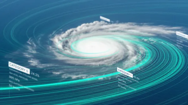 Today Google DeepMind and Google Research are launching a public preview of Weather Lab, an interactive website for sharing our AIweather models, and debuting our newest…
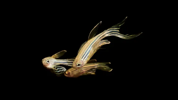 Learn how Google Research’s team worked with collaborators at HHMI Janelia and Harvard University to build a dataset that tracks both the neural activity and nanoscale s…