Posted by Elad Hazan and Yoram Singer, Research Scientists, Google AI and Princeton University

Google has long partnered with academia to advance research, collaborating with universities all over the world on joint research projects which result in novel developments in Computer Science, Engineering, and related fields. Today we announce the latest of these academic partnerships in the form of a new lab, across the street from Princeton University’s historic Nassau Hall, opening early next year. By fostering closer collaborations with faculty and students at Princeton, the lab aims to broaden research in multiple facets of machine learning, focusing its initial research efforts on optimization methods for large-scale machine learning, control theory and reinforcement learning. Below we give a brief overview of the research progress thus far.

Large-Scale Optimization
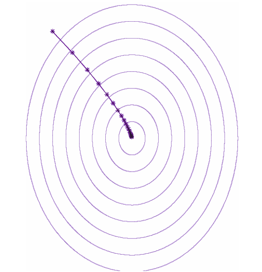
Imagine you have gone for a mountain hike and have run out of water. You need to get to a lake. How can you do so most efficiently? This is a matter of optimizing your route, and the mathematical analogue of this is the gradient descent method. You therefore move in the direction of steepest descent until you find the nearest lake at the bottom of your path. In the language of optimization, the location of the lake is referred to as a (local) minimum. The trajectory of gradient descent resembles the path, shown below, a thirsty yet avid hiker would take in order to get down to a lake as fast as she can.
Gradient descent (GD), and its randomized version, stochastic gradient descent (SGD), are the methods of choice for optimizing the weights of neural networks. Stacking all of the parameters together, we form a set of cells organized into vectors Let us take a simplistic view and assume that our neural net merely has 5 different parameters. Taking a gradient descent step amounts to subtracting the gradient vector (red) from the current set of parameters (blue) and putting the result back into the parameter vector.
Going back to our avid hiker, suppose she finds an unmarked path that is long and narrow, with limited visibility as she gazes down. If she follows the descent method her path would zig-zag down the hill, as shown in the illustration below on the left. However, she can now make faster progress by exploiting the skewed geometry of the terrain. That is, she can make a bigger leap forward than to the sides. In the context of gradient descent, pacing up is called acceleration. A popular class of acceleration methods is named adaptive regularization, or adaptive preconditioning, first introduced by the AdaGrad algorithm devised in collaboration with Prof. John Duchi from Stanford while he was at Google.
The idea is to change the geometry of the landscape of the optimization objective to make it easier for gradient descent to work. In order to do so, preconditioning methods stretch and rotate the space. The terrain after preconditioning looks like the serene, perfectly spherical lake above on the right, and the descent trajectory is a straight line! Procedurally, instead of subtracting the gradient vectors from the parameters vector per-se, adaptive preconditioning first multiplies the gradient by a 5×5 multicell structure, called a matrix preconditioner, as shown below.
This preconditioning operation yields a stretched and rotated gradient which is then subtracted as before, allowing much faster progress toward a basin. However, there is a downside to preconditioning, namely, its computational cost. Instead of subtracting a 5-dimensional gradient vector from a 5-dimensional parameter vector, the preconditioning transformation itself requires 5×5=25 operations. Suppose we would like to precondition gradients in order to learn a deep network with 10 million parameters. A single preconditioning step would require 100 trillion operations. In order to save computation, a diagonal version in which preconditioning amounts to stretching sans rotation was also introduced in the original AdaGrad paper. The diagonal version was later adopted and modified, yielding another very successful algorithm called Adam.

This simplified diagonal preconditioning imposes only a marginal additional cost to gradient descent. However, oversimplification has its own downside: we are no longer able to rotate our space. Going back to our hiker, if the deep-and-narrow canyon runs from southeast to northwest, she can no longer take large westward leaps. Had we provided her with a “rigged” compass in which the north pole is in the northwest, she could have followed her descent procedure as before. In high dimensions, the analog of compass rigging is full-matrix preconditioning. We thus asked ourselves whether we could devise a preconditioning method that is computationally efficient while allowing for the equivalent of coordinate rotations.

At Google AI Princeton, we developed a new method for full-matrix adaptive preconditioning at roughly the same computational cost as the commonly-used diagonal restriction. Details can be found in the paper, but the key idea behind the method is depicted below. Instead of using a full matrix, we replace the preconditioning matrix by a product of three matrices: a tall & thin matrix, a (small) square matrix, and a short & fat matrix. The vast amount of computation is performed using the smaller matrix. If we have d parameters, instead of a single large d × d matrix, the matrices maintained by GGT (shorthand for the operation Gradient Gradient^T), the proposed method, are of sizes d × k, k × k, k × d respectively.

For reasonable choices of k, which can be thought of as the “window size” of the algorithm, the computational bottleneck has been mitigated from a single large matrix, to that of a much smaller kkmatrix. In our implementation we typically choose k to be, say, 50, and maintaining the smaller square matrix is significantly less expensive while yielding good empirical performance. When compared to other adaptive methods on standard deep learning tasks, GGT is competitive with AdaGrad and Adam.

Spectral Filtering for Control and Reinforcement Learning
Another broad mission of Google’s research group in Princeton is to develop principled building blocks for decision-making systems. In particular, the group strives to leverage provable guarantees from the field of online learning, which studies the robust (worst-case) guarantees of decision-making algorithms under uncertainty. An online algorithm is said to attain a no-regret guarantee if it learns to make decisions as well as the best "offline" decision in hindsight. Ideas from this field have already enabled many innovations within theoretical computer science, and provide a mathematically elegant framework to study a widely-used technique called boosting. We envision using ideas from online learning to broaden the toolkit of modern reinforcement learning.

With that goal in mind, and in collaboration with researchers and students at Princeton, we developed the algorithmic technique of spectral filtering for estimation and control of linear dynamical systems (see several recent publications). In this setting, noisy observations (e.g., location sensor measurements) are being streamed from an unknown source. The source of the signal is a system whose state evolves over time following a set of linear equations (e.g. Newton's laws). To forecast future signals (prediction), or to perform actions which bring the system to a desired state (control), the usual approach starts with learning the model explicitly (a task termed system identification), which is often slow and inaccurate.

Spectral filtering circumvents the need to model the dynamics explicitly, by reformulating prediction and control as convex programs, enabling provable no-regret guarantees. A major component of the technique is that of a new signal processing transformation. The idea is to summarize the long history of past input signals through convolution with a tailored bank of filters, and then use this representation to predict the dynamical system’s future outputs. Each filter compresses the input signal into a single real number, by taking a weighted combination of the previous inputs.

A set of filters depicted in a plot of filter amplitude versus time. With our technique of spectral filtering, multiple filters are used to predict the state of a linear dynamical system at any given time. Each filter is a set of weights used to summarize past observations, such that combining them in a weighted fashion, over time allows us to accurately predict the system.

The mathematical derivation of these weights (filters) has an interesting connection to the spectral theory of Hankel matrices.

Looking Forward
We are excited about the progress we have made thus far in partnership with Princeton’s faculty and students, and we look forward to the official opening of the lab in the coming weeks. It has long been Google’s view that both industry and academia benefit significantly from an open research culture, and we look forward to our continued close collaboration.

Acknowledgments
The research and results discussed in this post would not have been possible without contributions from the following researchers: Naman Agarwal, Brian Bullins, Xinyi Chen, Udaya Ghai, Tomer Koren, Karan Singh, Cyril Zhang, Yi Zhang, and visiting professor Sham Kakade. Since joining Google earlier this year, the research team has been working remotely from both the Google NYC office as well as the Princeton University campus, and they look forward to moving into the new Google space across from the Princeton campus in the weeks to come.