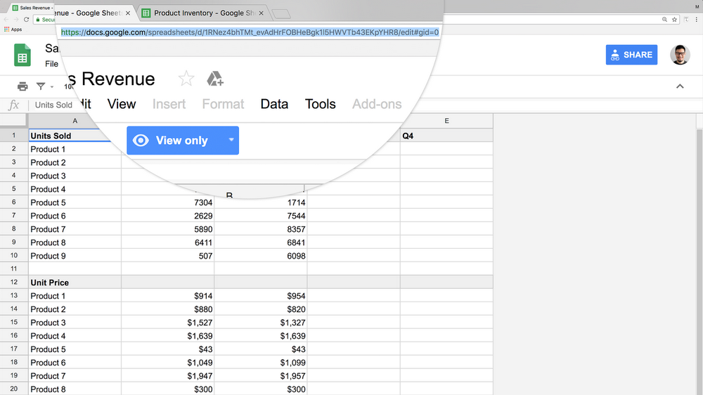
When it comes to analyzing data at work, we often have to pull information from several different sources in order to see the big picture. But if you need to manage product inventory or report on quarterly sales figures, spending time flipping between spreadsheets or manually copying and pasting data into one place can take up too much time. There’s a better option.
With G Suite—Google’s suite of cloud-based collaboration and productivity apps—there are a ton of ways you can skip repetitive tasks, including in Google Sheets.
Today, we’re kicking off a tips series to help you become a G Suite pro—starting with how to combine data from one spreadsheet into another. Check it out.
Combining data from two Google Sheets in four steps
With Sheets, it’s easy to combine data into one spreadsheet to create a single source of truth.
Step 1: Identify the spreadsheets you want to combine.
Pull up the two spreadsheets that you’d like to import data between. You should have the original spreadsheet (Ex: “Sales Revenue”) and the one you want to add information into (Ex: “Product Inventory”).
Step 2: Grab two things from the original sheet.
You need two pieces of information from the original spreadsheet in order to move the data: the spreadsheet URL and the range of cells where you want to pull the data from. In this example, our original spreadsheet’s name is “Sales Revenue.”
First, highlight and copy the full spreadsheet URL from the original spreadsheet (Note: you can also use the spreadsheet “key,” which is a code hidden inside the URL between the “d/” and “/edit.” It looks like a jumbled mix of letters and numbers.).

Next, before you switch to the new spreadsheet, make sure to note the range of cells where you want to pull the data from in the original spreadsheet. For example, A:1 to C:10.
Step 3: Use a Google Sheets function to port your data over.
Now we use the IMPORTRANGE function. First, click into the new spreadsheet where you’d like to add data into. In this example, it’s named “Product Inventory.” Insert columns or rows into the spreadsheet where you want to put data.
Next, type =IMPORTRANGE in the cell (you can choose to use all caps or not, it doesn’t matter.). The function will then ask you for three things:
- The URL of the original spreadsheet (or the spreadsheet key, both options work.)
- The name of the specific tab in your spreadsheet that you’re pulling information out of
- The range of cells for data you need
It will look similar to this:
=IMPORTRANGE(“https://docs.google.com/spreadsheets/d/1RNez4bhTMt_evAdHrFOBHeBgk1l5HAWVTb43EKpYHR8/edit#gid=0,””Sales Revenue by Quarter!A1:C10”)
It’s important to note that you have to use the specific name of the tab in the sheet in the formula. So for this example, the name of the original spreadsheet housing multiple datasets is called “Sales Revenue,” but the name of the specific tab with our data in it is called “Sales Revenue by Quarter.” We want to use the specific tab’s name to avoid our function breaking in the future when new sheets or tabs are created.
Oh and another trick: don’t forget to add the exclamation point (!) before the data range. That’s important, too.
Step 4: Import your data.
After you’ve added your IMPORTRANGE formula, you can click enter.
If it’s the first time you’ve imported data from that particular spreadsheet, a pop-up might appear. Don’t worry! This security check makes sure you’re okay with granting any collaborators on this spreadsheet access to data that lives in another spreadsheet. It will ask you to “Allow access” when you see the #REF in your cell. Go ahead and click yes.
Voilà! Your data will appear in the new spreadsheet.
