Tag Archives: AI for Social Good

Progress from a year of AI for Social Good at Google Research India

Almost a year and a half ago, we announced Google Research India, an AI Lab in Bangalore. Along with advancing fundamental research in AI, we sought  to support nonprofits and universities to solve big challenges in the field of Public Health, Conservation, Agriculture and Education using AI. 

In 2020, we announced AI for Social Good would be supporting six projects from NGOs and Academic collaborations to utilize the application of AI to assist underserved communities that have not traditionally benefited from the prowess of AI. Google provided scientific and technical contributions for each project, as well as  funding from Google Research and Google.org. 

Today, we are pleased to provide an update on some of these projects, and highlight successes and challenges in AI for Social Good. 

Maternal Healthcare

India accounts for 11 percent of global maternal mortality, and a woman in India dies in childbirth every fifteen minutes. However, almost 90 percent of maternal deaths are avoidable if women receive timely intervention. Access to timely, accurate health information is a significant challenge among women in rural areas and urban slums. ARMMAN runs mMitra, a free mobile voice call service that sends timely and targeted preventive care information to expectant and new mothers. Adherence to such public health programs is a big challenge but timely intervention to retain people is beneficial to improve maternal health outcomes. Researchers from Google Research and IIT Madras worked with ARMMAN to design an AI technology that could provide an indication of women who were at risk of dropping out from the health information program. The early targeted identification helps ARMMAN to personalise interventions and retain these people, improving maternal health outcomes. Test results demonstrated that use of AI technology was able to bring down the risk of drop-offs by up to 32% for women at high risk of dropping out. The team is currently working towards scaling this to 300,000+ women in mMitra and we are excited to continue to support ARMMAN as the project team increases the reach of this technology to 1M+ mothers and children in 2021. To support ARMMAN’s growing efforts, Google.org is committing another USD $530,000 to ARMMAN to scale the use of AI for social good to reach underserved women and children. 

The importance of targeted interventions to improve health outcomes cannot be overstated. AI can help play a critical role in its advancement, however the lack of availability of high-quality public health data is a significant challenge. Frequently, data collection is enabled through the labour and expertise of frontline health workers and yet Khushibaby discovered various challenges in the field that inhibited the collection of the high-quality data required. Researchers from Singapore Management University and Google Research collaborated with Khushibaby to develop AI algorithms with over 90 percent accuracy that provided timely predictions about the drop in health workers’ data quality. These timely predictions help Khushibaby provide assistance to the health worker to enable them to record high-quality data. The project team is currently planning to deploy and safely test this technology with 250+ healthcare workers who serve over 15,000 people. 

Wildlife Conservation

India is home to some of the most biodiverse regions, where human settlements and wildlife co-exist in forests. However, interactions between local communities and wildlife can result in conflicts, leading to loss of crops, cattle, and even human life. Wildlife Conservation Trust needed help to proactively predict human-wildlife conflict to enable them to take timely steps to protect local communities, wildlife, and the forest. With technical and scientific contributions from Google Research and Singapore Management University, Wildlife Conservation Trust designed AI models that help predict human-wildlife conflict in Bramhapuri Forest Division in Tadoba, Maharashtra. These novel AI techniques provide over 80 percent accuracy in predicting human-wildlife conflict in the Bramhapuri Forest Division in the test results. This work is currently being field-tested in Chandrapur district, Madhya Pradesh, to ensure safe deployment. 

Local Language Adoption

Six out of ten children globally do not achieve minimum proficiency levels in reading, despite attending school. Lack of access to reading content in one’s local language is a significant challenge in addressing this problem. Storyweaver, an open-licence driven organization, works towards bridging that gap by developing and curating story books in a multitude of local languages to help children learn new concepts, new ideas and open up their imagination.  Storyweaver needed help to enable access to creation tools in low-resource languages. Creation tools in low-resource languages suffer from very low accuracy, adding barriers to content creation. The team at AI4Bharat & IIT Madras, with support from Google, developed state-of-the-art Natural Language Understanding tools to develop open-language models for two low-resource languages (Konkani, Maithal), making story reading easier for 70,000+ children. 

We are humbled to see the progress in the development and deployment of AI technologies for social good in a short period of time. We are confident in our development and support of a collaborative model that involves experts from Academia and NGOs, as well as contributions from Google, to advance AI for social good. Continuing our scientific, technical, and financial support of organizations working in this space, we are excited to announce an expanded follow-up program to initiate collaborative AI for Social Good projects in Asia Pacific and Sub-Saharan Africa. 

We recognize that AI is not a magic wand to solve all the world’s challenges, it is however a powerful tool to help experts and social-impact organisations to explore and address hard, unanswered questions. 

Posted by Milind Tambe, Director of AI for Social Good, Google Research India, and Manish Gupta, Director, Google Research India


The Technology Behind our Recent Improvements in Flood Forecasting

Flooding is the most common natural disaster on the planet, affecting the lives of hundreds of millions of people around the globe and causing around $10 billion in damages each year. Building on our work in previous years, earlier this week we announced some of our recent efforts to improve flood forecasting in India and Bangladesh, expanding coverage to more than 250 million people, and providing unprecedented lead time, accuracy and clarity.

To enable these breakthroughs, we have devised a new approach for inundation modeling, called a morphological inundation model, which combines physics-based modeling with machine learning (ML) to create more accurate and scalable inundation models in real-world settings. Additionally, our new alert-targeting model allows identifying areas at risk of flooding at unprecedented scale using end-to-end machine learning models and data that is publicly available globally. In this post, we also describe developments for the next generation of flood forecasting systems, called HydroNets (presented at ICLR AI for Earth Sciences and EGU this year), which is a new architecture specially built for hydrologic modeling across multiple basins, while still optimizing for accuracy at each location.

Forecasting Water Levels
The first step in a flood forecasting system is to identify whether a river is expected to flood. Hydrologic models (or gauge-to-gauge models) have long been used by governments and disaster management agencies to improve the accuracy and extend the lead time of their forecasts. These models receive inputs like precipitation or upstream gauge measurements of water level (i.e., the absolute elevation of the water above sea level) and output a forecast for the water level (or discharge) in the river at some time in the future.

The hydrologic model component of the flood forecasting system described in this week’s Keyword post doubled the lead time of flood alerts for areas covering more than 75 million people. These models not only increase lead time, but also provide unprecedented accuracy, achieving an R2 score of more than 99% across all basins we cover, and predicting the water level within a 15 cm error bound more than 90% of the time. Once a river is predicted to reach flood level, the next step in generating actionable warnings is to convert the river level forecast into a prediction for how the floodplain will be affected.

Morphological Inundation Modeling
In prior work, we developed high quality elevation maps based on satellite imagery, and ran physics-based models to simulate water flow across these digital terrains, which allowed warnings with unprecedented resolution and accuracy in data-scarce regions. In collaboration with our satellite partners, Airbus, Maxar and Planet, we have now expanded the elevation maps to cover hundreds of millions of square kilometers. However, in order to scale up the coverage to such a large area while still retaining high accuracy, we had to re-invent how we develop inundation models.

Inundation modeling estimates what areas will be flooded and how deep the water will be. This visualization conceptually shows how inundation could be simulated, how risk levels could be defined (represented by red and white colors), and how the model could be used to identify areas that should be warned (green dots).

Inundation modeling at scale suffers from three significant challenges. Due to the large areas involved and the resolution required for such models, they necessarily have high computational complexity. In addition, most global elevation maps don’t include riverbed bathymetry, which is important for accurate modeling. Finally, the errors in existing data, which may include gauge measurement errors, missing features in the elevation maps, and the like, need to be understood and corrected. Correcting such problems may require collecting additional high-quality data or fixing erroneous data manually, neither of which scale well.

Our new approach to inundation modeling, which we call a morphological model, addresses these issues by using several innovative tricks. Instead of modeling the complex behaviors of water flow in real time, we compute modifications to the morphology of the elevation map that allow one to simulate the inundation using simple physical principles, such as those describing hydrostatic systems.

First, we train a pure-ML model (devoid of physics-based information) to estimate the one-dimensional river profile from gauge measurements. The model takes as input the water level at a specific point on the river (the stream gauge) and outputs the river profile, which is the water level at all points in the river. We assume that if the gauge increases, the water level increases monotonically, i.e., the water level at other points in the river increases as well. We also assume that the absolute elevation of the river profile decreases downstream (i.e., the river flows downhill).

We then use this learned model and some heuristics to edit the elevation map to approximately “cancel out” the pressure gradient that would exist if that region were flooded. This new synthetic elevation map provides the foundation on which we model the flood behavior using a simple flood-fill algorithm. Finally, we match the resulting flooded map to the satellite-based flood extent with the original stream gauge measurement.

This approach abandons some of the realistic constraints of classical physics-based models, but in data scarce regions where existing methods currently struggle, its flexibility allows the model to automatically learn the correct bathymetry and fix various errors to which physics-based models are sensitive. This morphological model improves accuracy by 3%, which can significantly improve forecasts for large areas, while also allowing for much more rapid model development by reducing the need for manual modeling and correction.

Alert targeting
Many people reside in areas that are not covered by the morphological inundation models, yet access to accurate predictions are still urgently needed. To reach this population and to increase the impact of our flood forecasting models, we designed an end-to-end ML-based approach, using almost exclusively data that is globally publicly available, such as stream gauge measurements, public satellite imagery, and low resolution elevation maps. We train the model to use the data it is receiving to directly infer the inundation map in real time.

A direct ML approach from real-time measurements to inundation.

This approach works well “out of the box” when the model only needs to forecast an event that is within the range of events previously observed. Extrapolating to more extreme conditions is much more challenging. Nevertheless, proper use of existing elevation maps and real-time measurements can enable alerts that are more accurate than presently available for those in areas not covered by the more detailed morphological inundation models. Because this model is highly scalable, we were able to launch it across India after only a few months of work, and we hope to roll it out to many more countries soon.

Improving Water Levels Forecasting
In an effort to continue improving flood forecasting, we have developed HydroNets — a specialized deep neural network architecture built specifically for water levels forecasting — which allows us utilize some exciting recent advances in ML-based hydrology in a real-world operational setting. Two prominent features distinguish it from standard hydrologic models. First, it is able to differentiate between model components that generalize well between sites, such as the modeling of rainfall-runoff processes, and those that are specific to a given site, like the rating curve, which converts a predicted discharge volume into an expected water level. This enables the model to generalize well to different sites, while still fine-tuning its performance to each location. Second, HydroNets takes into account the structure of the river network being modeled, by training a large architecture that is actually a web of smaller neural networks, each representing a different location along the river. This allows neural networks that are modeling upstream sites to pass information encoded in embeddings to models of downstream sites, so that every model can know everything it needs without a drastic increase in parameters.

The animation below illustrates the structure and flow of information in HydroNets. The output from the modeling of upstream sub-basins is combined into a single representation of a given basin state. It is then processed by the shared model component, which is informed by all basins in the network, and passed on to the label prediction model, which calculates the water level (and the loss function). The output from this iteration of the network is then passed on to inform downstream models, and so on.

An illustration of the HydroNets architecture.

We’re incredibly excited about this progress, and are working hard on improving our systems further.

Acknowledgements
This work is a collaboration between many research teams at Google, and is part of our AI for Social Good efforts. We'd also like to thank our Geo and Policy teams, as well as Google.org.

Source: Google AI Blog


Leveraging Temporal Context for Object Detection


Ecological monitoring helps researchers to understand the dynamics of global ecosystems, quantify biodiversity, and measure the effects of climate change and human activity, including the efficacy of conservation and remediation efforts. In order to monitor effectively, ecologists need high-quality data, often expending significant efforts to place monitoring sensors, such as static cameras, in the field. While it is increasingly cost effective to build and operate networks of such sensors, the manual data analysis of global biodiversity data remains a bottleneck to accurate, global, real-time ecological monitoring. While there are ways to automate this analysis via machine learning, the data from static cameras, widely used to monitor the world around us for purposes ranging from mountain pass road conditions to ecosystem phenology, still pose a strong challenge for traditional computer vision systems — due to power and storage constraints, sampling frequencies are low, often no faster than one frame per second, and sometimes are irregular due to the use of a motion trigger.

In order to perform well in this setting, computer vision models must be robust to objects of interest that are often off-center, out of focus, poorly lit, or at a variety of scales. In addition, a static camera will always take images of the same scene unless it is moved, which causes the data from any one camera to be highly repetitive. Without sufficient data variability, machine learning models may learn to focus on correlations in the background, leading to poor generalization to novel deployments. The machine learning and ecological communities have been working together through venues like LILA BC and Wildlife Insights to curate expert-labeled training data from many research groups, each of which may operate anywhere from one to hundreds of camera traps, in order to increase data variability. This process of data collection and annotation is slow, and is confounded by the need to have diverse, representative data across geographic regions and taxonomic groups.
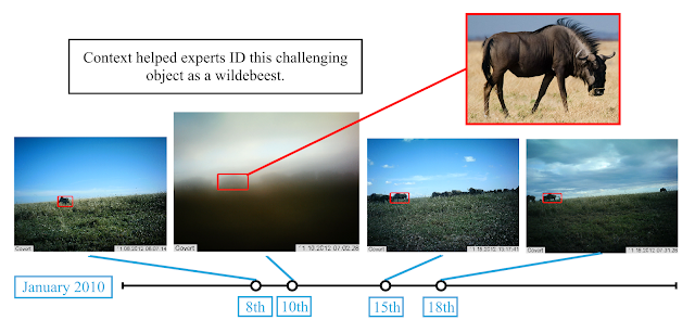
What’s in this image? Objects in images from static cameras can be very challenging to detect and categorize. Here, a foggy morning has made it very difficult to see a herd of wildebeest walking along the crest of a hill. [Image from Snapshot Serengeti]
In Context R-CNN: Long Term Temporal Context for Per-Camera Object Detection, we present a complementary approach that increases global scalability by improving generalization to novel camera deployments algorithmically. This new object detection architecture leverages contextual clues across time for each camera deployment in a network, improving recognition of objects in novel camera deployments without relying on additional training data from a large number of cameras. Echoing the approach a person might use when faced with challenging images, Context R-CNN leverages up to a month’s worth of images from the same camera for context to determine what objects might be present and identify them. Using this method, the model outperforms a single-frame Faster R-CNN baseline by significant margins across multiple domains, including wildlife camera traps. We have open sourced the code and models for this work as part of the TF Object Detection API to make it easy to train and test Context R-CNN models on new static camera datasets.
Here, we can see how additional examples from the same scene help experts determine that the object is an animal and not background. Context such as the shape & size of the object, its attachment to a herd, and habitual grazing at certain times of day help determine that the species is a wildebeest. Useful examples occur throughout the month.
The Context R-CNN Model
Context R-CNN is designed to take advantage of the high degree of correlation within images taken by a static camera to boost performance on challenging data and improve generalization to new camera deployments without additional human data labeling. It is an adaptation of Faster R-CNN, a popular two-stage object detection architecture. To extract context for a camera, we first use a frozen feature extractor to build up a contextual memory bank from images across a large time horizon (up to a month or more). Next, objects are detected in each image using Context R-CNN which aggregates relevant context from the memory bank to help detect objects under challenging conditions (such as the heavy fog obscuring the wildebeests in our previous example). This aggregation is performed using attention, which is robust to the sparse and irregular sampling rates often seen in static monitoring cameras.
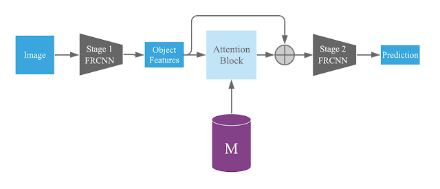
High-level architecture diagram, showing how Context R-CNN incorporates long-term context within the Faster R-CNN model architecture.
The first stage of Faster R-CNN proposes potential objects, and the second stage categorizes each proposal as either background or one of the target classes. In Context R-CNN, we take the proposed objects from the first stage of Faster R-CNN, and for each one we use similarity-based attention to determine how relevant each of the features in our memory bank (M) is to the current object, and construct a per-object context feature by taking a relevance-weighted sum over M and adding it back to the original object features. Then each object, now with added contextual information, is finally categorized using the second stage of Faster R-CNN.
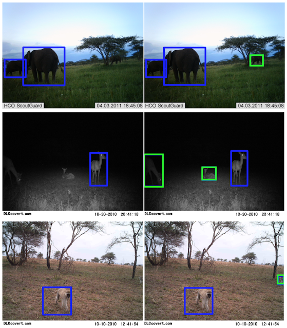
Context R-CNN is able to leverage context (spanning up to 1 month) to correctly categorize the challenging wildebeest example we saw above. The green values are the corresponding attention weights for each boxed object.
Compared to a Faster R-CNN baseline (left), Context R-CNN (right) is able to capture challenging objects such as an elephant occluded by a tree, two poorly-lit impala, and a vervet monkey leaving the frame. [Images from Snapshot Serengeti]
Results
We have tested Context R-CNN on Snapshot Serengeti (SS) and Caltech Camera Traps (CCT), both ecological datasets of animal species in camera traps but from highly different geographic regions (Tanzania vs. the Southwestern United States). Improvements over the Faster R-CNN baseline for each dataset can be seen in the table below. Notably, we see a 47.5% relative increase in mean average precision (mAP) on SS, and a 34.3% relative mAP increase on CCT. We also compare Context R-CNN to S3D (a 3D convolution based baseline) and see performance improve from 44.7% mAP to 55.9% mAP (a 25.1% relative increase). Finally, we find that the performance increases as the contextual time horizon increases, from a minute of context to a month.
Comparison to a single frame Faster R-CNN baseline, showing both mean average precision (mAP) and average recall (AR) detection metrics.
Ongoing and Future Work
We are working to implement Context R-CNN within the Wildlife Insights platform, to facilitate large-scale, global ecological monitoring via camera traps. We also host competitions such as the yearly iWildCam species identification competition at the CVPR Fine-Grained Visual Recognition Workshop to help bring these challenges to the attention of the computer vision community. The challenges seen in automatic species identification in static cameras are shared by numerous applications of static cameras outside of the ecological monitoring domain, as well as other static sensors used to monitor biodiversity, such as audio and sonar devices. Our method is general, and we anticipate the per-sensor context approach taken by Context R-CNN would be beneficial for any static sensor.

Acknowledgements
This post reflects the work of the authors as well as the following group of core contributors: Vivek Rathod, Guanhang Wu, Ronny Votel. We are also grateful to Zhichao Lu, David Ross, Tanya Birch and the Wildlife Insights AI team, and Pietro Perona and the Caltech Computational Vision Lab.

Source: Google AI Blog


Machine Learning-based Damage Assessment for Disaster Relief


Natural disasters, such as earthquakes, hurricanes, and floods, affect large areas and millions of people, but responding to such disasters is a massive logistical challenge. Crisis responders, including governments, NGOs, and UN organizations, need fast access to comprehensive and accurate assessments in the aftermath of disasters to plan how best to allocate limited resources.To this end, very high resolution (VHR) satellite imagery, with up to 0.3 meter resolution, is becoming an increasingly important tool for crisis response, giving responders an unprecedented breadth of visual information about how terrain, infrastructure, and populations are changed by disasters.

However, intensive manual labor is still required to extract operationally-relevant information — collapsed buildings, cracks in bridges, where people have set up temporary shelters — from the raw satellite imagery. As an example, for the 2010 Haiti earthquake, analysts manually examined over 90,000 buildings in the Port-au-Prince area alone, rating the damage each one incurred on a five point scale. Many of these manual analyses take teams of experts many weeks to complete, whereas they are most needed within 48-72 hours after the disaster, when the most urgent decisions are made.

To help mitigate the impact of such disasters, we present "Building Damage Detection in Satellite Imagery Using Convolutional Neural Networks", which details a machine learning (ML) approach to automatically process satellite data to generate building damage assessments. Developed in partnership with the United Nations World Food Program (WFP) Innovation Accelerator, we believe this work has the potential to drastically reduce the time and effort required for crisis workers to produce damage assessment reports. In turn, this would reduce the turnaround times needed to deliver timely disaster aid to the most severely affected areas, while increasing the overall coverage of such critical services.

The Approach
The automatic damage assessment process is split into two steps: building detection and damage classification. In the building detection step, our approach uses an object detection model to draw bounding boxes around each building in the image. We then extract pre-disaster and post-disaster images centered on each detected building and use a classification model to determine whether the building is damaged.

The classification model consists of a convolutional neural network to which is input two 161 pixel x 161 pixel RGB images, corresponding to a 50 m x 50 m ground footprint, centered on a given building. One image is from before the disaster event, and the other image is from after the disaster event. The model analyzes differences in the two images and outputs a score from 0.0 to 1.0, where 0.0 means the building was not damaged, and 1.0 means the building was damaged.

Because the before and after images are taken on different dates, at different times of day, and in some cases by different satellites altogether, there can be a host of different problems that arise. For example, the brightness, contrast, color saturation, and lighting conditions of the images may differ significantly, and the pixels in the image may be misaligned.

To correct for differences in color and illumination, we use histogram equalization to normalize the colors in the before and after images. We also make the model more robust to insignificant color differences by using standard data augmentation techniques, such as randomly perturbing the contrast and saturation of the images, during training.

Training Data
One of the main challenges of this work is assembling a training data set. Data availability in this application is inherently limited because there are only a handful of disasters that have high resolution satellite images and an even smaller number that have existing damage assessments. For labels, we use publicly available damage assessments manually generated by humanitarian organizations operating in this space, such as UNOSAT and REACH. We obtain the original satellite images on which the manual assessments are performed and then use Google Earth Engine to spatially join the damage assessment labels with the satellite images in order to produce the final training examples. All images used to train the model were sourced from commercially available sources.
Examples of individual image patches that capture before and after images of damaged and undamaged buildings from different disasters.
Results
We evaluated this technology for 3 major past earthquakes: the 2010 earthquake in Haiti (magnitude 7.0), the 2017 event in Mexico City (magnitude 7.1), and the series of earthquakes occuring in Indonesia in 2018 (magnitudes 5.9 - 7.5). For each event, we trained the model on buildings in one part of the region affected by the quake and tested it on buildings in another part of the region. We used human expert damage assessments performed by UNOSAT and REACH as the ground truth for evaluation. We measure the model’s quality using both true accuracy (compared to expert assessment) and the area under the ROC curve (AUROC), which captures the trade-off between the model’s true positive and false positive rates of detection, and is a common way to measure quality when the number of positive and negative examples in the test dataset is imbalanced. An AUROC value of 0.5 means that the model’s predictions are random, while a value of 1.0 means the model is perfectly accurate. According to crisis responder feedback, 70% accuracy is the threshold needed for making high-level decisions in the first 72 hours after the disaster.
Area under the
Event Accuracy ROC curve
2010 Haiti earthquake 77% 0.83
2017 Mexico City earthquake 71% 0.79
2018 Indonesia earthquake 78% 0.86
Evaluation of model predictions against human expert assessments (higher is better).
Example model predictions from the 2010 Haiti earthquake. Prediction values closer to 1.0 means the model is more confident that the building is damaged. Values closer to 0.0 means the building is not damaged. A threshold value of 0.5 is typically used to distinguish between damaged/undamaged predictions, but this can be tuned to make the predictions more or less sensitive.
Future Work
While the current model works reasonably well when trained and tested on buildings from the same regions (e.g., same city or country), the ultimate goal is to have a model that can accurately assess building damage for disasters that happen anywhere in the world, and not just those that look similar to the ones the model has been trained on. This is challenging because the variety of the available training data for past disasters is inherently limited to a handful of events that occurred in a few geographic locations. Generalizing to future disasters that will likely occur in new locations is therefore still a challenge for our model and is the focus of ongoing work. We envision a system that can be interactively trained, validated, and deployed by expert analysts so that important aid distribution decisions are always verified by experienced crisis responders. Our hope is that this technology can help communities get the aid that they need in times of most critical need in a timely fashion.

Acknowledgements
This post reflects the work of our co-authors Wenhan Lu and Zebo Li. We would also like to thank Maolin Zuo for his contributions to the project. In tackling this problem, we have had a very productive partnership with the United Nations World Food Programme (WFP) Innovation Accelerator, an organization that identifies, funds, and supports startups and innovative projects to disrupt world hunger.

Source: Google AI Blog


A Neural Weather Model for Eight-Hour Precipitation Forecasting


Predicting weather from minutes to weeks ahead with high accuracy is a fundamental scientific challenge that can have a wide ranging impact on many aspects of society. Current forecasts employed by many meteorological agencies are based on physical models of the atmosphere that, despite improving substantially over the preceding decades, are inherently constrained by their computational requirements and are sensitive to approximations of the physical laws that govern them. An alternative approach to weather prediction that is able to overcome some of these constraints uses deep neural networks (DNNs): instead of encoding explicit physical laws, DNNs discover patterns in the data and learn complex transformations from inputs to the desired outputs using parallel computation on powerful specialized hardware such as GPUs and TPUs.

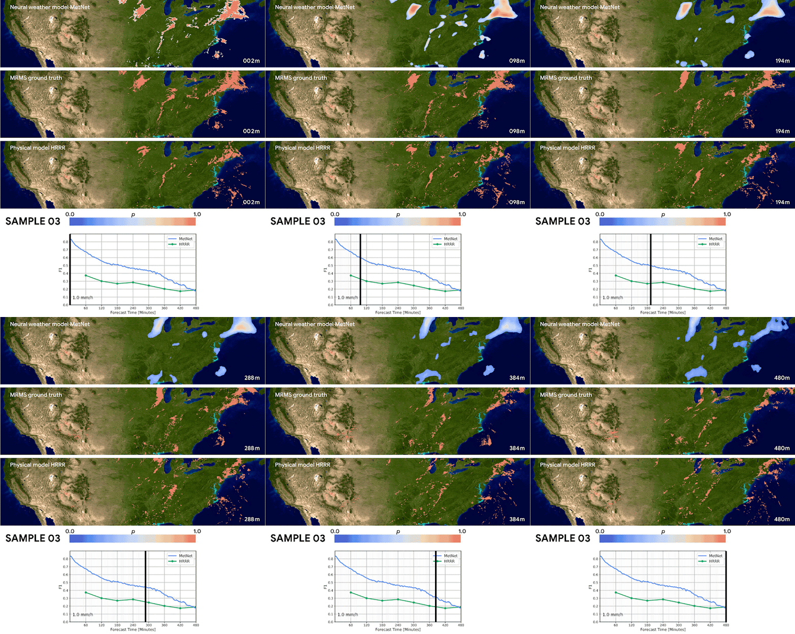
Building on our previous research into precipitation nowcasting, we present “MetNet: A Neural Weather Model for Precipitation Forecasting,” a DNN capable of predicting future precipitation at 1 km resolution over 2 minute intervals at timescales up to 8 hours into the future. MetNet outperforms the current state-of-the-art physics-based model in use by NOAA for prediction times up to 7-8 hours ahead and makes a prediction over the entire US in a matter of seconds as opposed to an hour. The inputs to the network are sourced automatically from radar stations and satellite networks without the need for human annotation. The model output is a probability distribution that we use to infer the most likely precipitation rates with associated uncertainties at each geographical region. The figure below provides an example of the network’s predictions over the continental United States.
MetNet model predictions compared to the ground truth as measured by the NOAA multi-radar/multi-sensor system (MRMS). The MetNet model (top) displays the probabilities for 1 mm/hr precipitation predicted from 2 minutes to 480 minutes ahead, whereas the MRMS data (bottom) shows the areas receiving at least 1 mm/hr of precipitation over that same time period.
Neural Weather Model
MetNet does not rely on explicit physical laws describing the dynamics of the atmosphere, but instead learns by backpropagation to forecast the weather directly from observed data. The network uses precipitation estimates derived from ground based radar stations comprising the multi-radar/multi-sensor system (MRMS) and measurements from NOAA’s Geostationary Operational Environmental Satellite system that provides a top down view of clouds in the atmosphere. Both data sources cover the continental US and provide image-like inputs that can be efficiently processed by the network.

The model is executed for every 64 km x 64 km square covering the entire US at 1 km resolution. However, the actual physical coverage of the input data corresponding to each of these output regions is much larger, since it must take into account the possible motion of the clouds and precipitation fields over the time period for which the prediction is made. For example, assuming that clouds move up to 60 km/h, in order to make informed predictions that capture the temporal dynamics of the atmosphere up to 8 hours ahead, the model needs 60 x 8 = 480 km of spatial context in all directions. So, to achieve this level of context, information from a 1024 km x 1024 km area is required for predictions being made on the center 64 km x 64 km patch.
Size of the input patch containing satellite and radar images (large, 1024 x 1024 km square) and of the output predicted radar image (small, 64 x 64 km square).
Because processing a 1024 km x 1024 km area at full resolution requires a significant amount of memory, we use a spatial downsampler that decreases memory consumption by reducing the spatial dimension of the input patch, while also finding and keeping the relevant weather patterns in the input. A temporal encoder (implemented with a convolutional LSTM that is especially well suited for sequences of images) is then applied along the time dimension of the downsampled input data, encoding seven snapshots from the previous 90 minutes of input data, in 15-minute segments. The output of the temporal encoder is then passed to a spatial aggregator, which uses axial self-attention to efficiently capture long range spatial dependencies in the data, with a variable amount of context based on the input target time, to make predictions over the 64 km x 64 km output.

The output of this architecture is a discrete probability distribution estimating the probability of a given rate of precipitation for each square kilometer in the continental United States.
The architecture of the neural weather model, MetNet. The input satellite and radar images first pass through a spatial downsampler to reduce memory consumption. They are then processed by a convolutional LSTM at 15 minute intervals over the 90 minutes of input data. Then axial attention layers are used to make the network see the entirety of the input images.
Results
We evaluate MetNet on a precipitation rate forecasting benchmark and compare the results with two baselines — the NOAA High Resolution Rapid Refresh (HRRR) system, which is the physical weather forecasting model currently operational in the US, and a baseline model that estimates the motion of the precipitation field (i.e., optical flow), a method known to perform well for prediction times less than 2 hours.

A significant advantage of our neural weather model is that it is optimized for dense and parallel computation and well suited for running on specialty hardware (e.g., TPUs). This allows predictions to be made in parallel in a matter of seconds, whether it is for a specific location like New York City or for the entire US, whereas physical models such as HRRR have a runtime of about an hour on a supercomputer.

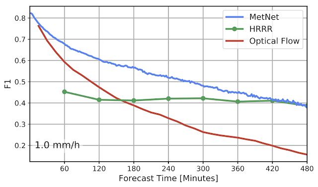
We quantify the difference in performance between MetNet, HRRR, and the optical flow baseline model in the plot below. Here, we show the performance achieved by the three models, evaluated using the F1-score at a precipitation rate threshold of 1.0 mm/h, which corresponds to light rain. The MetNet neural weather model is able to outperform the NOAA HRRR system at timelines less than 8 hours and is consistently better than the flow-based model.
Performance evaluated in terms of F1-score at 1.0 mm/h precipitation rate (higher is better). The neural weather model (MetNet) outperforms the physics-based model (HRRR) currently operational in the US for timescales up to 8 hours ahead.
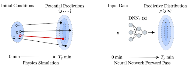
Due to the stochastic nature of the atmosphere, the uncertainty about the exact future weather conditions increases with longer prediction times. Because MetNet is a probabilistic model, the uncertainty in the predictions is seen in the visualizations by the growing smoothness of the predictions as the forecast time is extended. In contrast, HRRR does not directly make probabilistic predictions, but instead predicts a single potential future. The figure below compares the output of the MetNet model to that of the HRRR model.
Comparison between the output from MetNet (top) and HRRR (bottom) to ground-truth (middle) as retrieved from the NOAA MRMS system. Notice that while the HRRR model predicts structure that appears to be more similar to that of the ground-truth, the structure predicted may be grossly incorrect.
The predictions from the HRRR physical model look sharper and more structured than that of the MetNet model, but the structure, specifically the exact time and location where the structure is predicted, is less accurate due to uncertainty in the initial conditions and the parameters of the model.
HRRR (left) predicts a single potential future outcome (in red) out of the many possible outcomes, whereas MetNet (right) directly accounts for uncertainty by assigning probabilities over the future outcomes.
A more thorough comparison between the HRRR and MetNet models can be found in the video below:
Future Directions
We are actively researching how to improve global weather forecasting, especially in regions where the impacts of rapid climate change are most profound. While we demonstrate the present MetNet model for the continental US, it could be extended to cover any region for which adequate radar and optical satellite data are available. The work presented here is a small stepping stone in this effort that we hope leads to even greater improvements through future collaboration with the meteorological community.

Acknowledgements
This project was done in collaboration with Lasse Espeholt, Jonathan Heek, Mostafa Dehghani, Avital Oliver, Tim Salimans, Shreya Agrawal and Jason Hickey. We would also like to thank Manoj Kumar, Wendy Shang, Dick Weissenborn, Cenk Gazen, John Burge, Stephen Hoyer, Lak Lakshmanan, Rob Carver, Carla Bromberg and Aaron Bell for useful discussions and Tom Small for help with the visualizations.

Source: Google AI Blog


Using Machine Learning to “Nowcast” Precipitation in High Resolution


The weather can affect a person’s daily routine in both mundane and serious ways, and the precision of forecasting can strongly influence how they deal with it. Weather predictions can inform people about whether they should take a different route to work, if they should reschedule the picnic planned for the weekend, or even if they need to evacuate their homes due to an approaching storm. But making accurate weather predictions can be particularly challenging for localized storms or events that evolve on hourly timescales, such as thunderstorms.

In “Machine Learning for Precipitation Nowcasting from Radar Images,” we are presenting new research into the development of machine learning models for precipitation forecasting that addresses this challenge by making highly localized “physics-free” predictions that apply to the immediate future. A significant advantage of machine learning is that inference is computationally cheap given an already-trained model, allowing forecasts that are nearly instantaneous and in the native high resolution of the input data. This precipitation nowcasting, which focuses on 0-6 hour forecasts, can generate forecasts that have a 1km resolution with a total latency of just 5-10 minutes, including data collection delays, outperforming traditional models, even at these early stages of development.

Moving Beyond Traditional Weather Forecasting
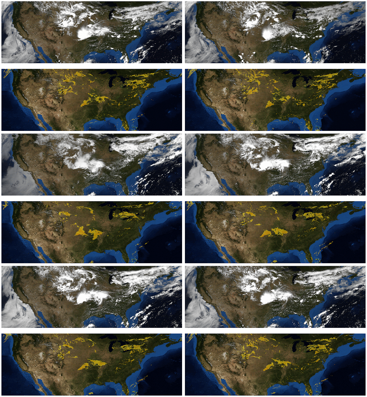
Weather agencies around the world have extensive monitoring facilities. For example, Doppler radar measures precipitation in real-time, weather satellites provide multispectral imaging, ground stations measure wind and precipitation directly, etc. The figure below, which compares false-color composite radar imaging of precipitation over the continental US to cloud cover imaged by geosynchronous satellites, illustrates the need for multi-source weather information. The existence of rain is related to, but not perfectly correlated with, the existence of clouds, so inferring precipitation from satellite images alone is challenging.
Top: Image showing the location of clouds as measured by geosynchronous satellites. Bottom: Radar image showing the location of rain as measured by Doppler radar stations. (Credit: NOAA, NWS, NSSL)
Unfortunately, not all of these measurements are equally present across the globe. For example, radar data comes largely from ground stations and is generally not available over the oceans. Further, coverage varies geographically, and some locations may have poor radar coverage even when they have good satellite coverage.

Even so, there is so much observational data in so many different varieties that forecasting systems struggle to incorporate it all. In the US, remote sensing data collected by the National Oceanic and Atmospheric Administration (NOAA) is now reaching 100 terabytes per day. NOAA uses this data to feed the massive weather forecasting engines that run on supercomputers to provide 1- to 10-day global forecasts. These engines have been developed over the course of the last half century, and are based on numerical methods that directly simulate physical processes, including atmospheric dynamics and numerous effects like thermal radiation, vegetation, lake and ocean effects, and more.

However, the availability of computational resources limits the power of numerical weather prediction in several ways. For example, computational demands limit the spatial resolution to about 5 kilometers, which is not sufficient for resolving weather patterns within urban areas and agricultural land. Numerical methods also take multiple hours to run. If it takes 6 hours to compute a forecast, that allows only 3-4 runs per day and resulting in forecasts based on 6+ hour old data, which limits our knowledge of what is happening right now. By contrast, nowcasting is especially useful for immediate decisions from traffic routing and logistics to evacuation planning.

Radar-to-Radar Forecasting
As a typical example of the type of predictions our system can generate, consider the radar-to-radar forecasting problem: given a sequence of radar images for the past hour, predict what the radar image will be N hours from now, where N typically ranges from 0-6 hours. Since radar data is organized into images, we can pose this prediction as a computer vision problem, inferring the meteorological evolution from the sequence of input images. At these short timescales, the evolution is dominated by two physical processes: advection for the cloud motion, and convection for cloud formation, both of which are significantly affected by local terrain and geography.
Top (left to right): The first three panels show radar images from 60 minutes, 30 minutes, and 0 minutes before now, the point at which a prediction is desired. The right-most panel shows the radar image 60 minutes after now, i.e., the ground truth for a nowcasting prediction. Bottom Left: For comparison, a vector field induced from applying an optical flow (OF) algorithm for modeling advection to the data from the first three panels above. Optical flow is a computer vision method that was developed in the 1940s, and is frequently used to predict short term weather evolution. Bottom Right: An example prediction made by OF. Notice that it tracks the motion of the precipitation in the bottom left corner well, but fails to account for the decaying strength of the storm.
We use a data-driven physics-free approach, meaning that the neural network will learn to approximate the atmospheric physics from the training examples alone, not by incorporating a priori knowledge of how the atmosphere actually works. We treat weather prediction as an image-to-image translation problem, and leverage the current state-of-the-art in image analysis: convolutional neural networks (CNNs).

CNNs are usually composed of a linear sequence of layers, where each layer is a set of operations that transform some input image into a new output image. Often, a layer will change the number of channels and the overall resolution of the image it’s given, in addition to convolving the image with a set of convolutional filters. These filters are themselves small images (for us, they are typically only 3x3, or 5x5). Filters drive much of the power of CNNs, and result in operations like detecting edges, identifying meaningful patterns, etc.

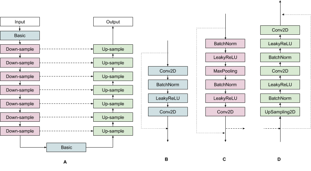
A particularly effective type of CNN is the U-Net. U-Nets have a sequence of layers that are arranged in an encoding phase, in which layers iteratively decrease the resolution of the images passing through them, and then a decoding phase in which the low-dimensional representations of the image created by the encoding phase are expanded back to higher resolutions. The following figure shows all of the layers in our particular U-Net.
(A) The overall structure of our U-NET. Blue boxes correspond to basic CNN layers. Pink boxes correspond to down-sample layers. Green boxes correspond to up-sample layers. Solid lines indicate input connections between layers. Dashed lines indicate long skip connections transversing the encoding and decoding phases of the U-NET. Dotted lines indicate short skip connections for individual layers. (B) The operations within our basic layer. (C) The operations within our down-sample layers. (D) The operations within our up-sample layers.
The input to the U-Net is an image that contains one channel for each multispectral satellite image in the sequence of observations over the last hour. For example, if there were 10 satellite images collected in the last hour, and each of those multispectral images was taken at 10 different wavelengths, then the image input for our model would be an image with 100 channels. For radar-to-radar forecasting, the input is a sequence of 30 radar observations over the past hour, spaced 2 minutes apart, and the output contains the prediction for N hours from now. For our initial work in the US, we trained a network from historical observations over the continental US from the period between 2017 and 2019. The data is split into periods of four weeks, where the first three weeks of each period are used for training and the fourth week is used for evaluation.

Results
We compare our results with three widely used models. First, the High Resolution Rapid Refresh (HRRR) numerical forecast from NOAA. HRRR actually contains predictions for many different weather quantities. We compared our results to their 1-hour total accumulated surface precipitation prediction, as that was their highest quality 1-hour precipitation prediction. Second, an optical flow (OF) algorithm, which attempts to track moving objects through a sequence of images. This latter approach is often applied to weather prediction even though it makes the assumption that overall rain quantities over large areas are constant over the prediction time — an assumption that is clearly violated. Third, the so-called persistence model, is the trivial model in which each location is assumed to be raining in the future at the same rate it is raining now, i.e. the precipitation pattern does not change. That may seem like an overly simplistic model to compare to, but it is common practice given the difficulty of weather prediction.
A visualization of predictions made over the course of roughly one day. Left: The 1-hour HRRR prediction made at the top of each hour, the limit to how often HRRR provides predictions. Center: The ground truth, i.e., what we are trying to predict. Right: The predictions made by our model. Our predictions are every 2 minutes (displayed here every 15 minutes) at roughly 10 times the spatial resolution made by HRRR. Notice that we capture the general motion and general shape of the storm.
We use precision and recall (PR) graphs to compare the models. Since we have direct access to our own classifier, we provide a full PR curve (seen as the blue line in the figure below). However, since we don’t have direct access to the HRRR model, and since neither the persistence model nor OF have the ability to trade-off precision and recall, those models are represented only by individual points. As can be seen, the quality of our neural network forecast outperforms all three of these models (since the blue line is above all of the other model’s results). It is important to note, however, that the HRRR model begins to outperform our current results when the prediction horizon reaches roughly 5 to 6 hours.
Precision and recall (PR) curves comparing our results (solid blue line) with: optical flow (OF), the persistence model, and the HRRR 1-hour prediction. As we do not have direct access to their classifiers, we cannot provide a full PR curve for their results. Left: Predictions for light rain. Right: Predictions for moderate rain.
One of the advantages of the ML method is that predictions are effectively instantaneous, meaning that our forecasts are based on fresh data, while HRRR is hindered by computational latency of 1-3 hours. This leads to better forecasts for computer vision methods for very short term forecasting. In contrast, the numerical model used in HRRR can make better long term predictions, in part because it uses a full 3D physical model — cloud formation is harder to observe from 2D images, and so it is harder for ML methods to learn convective processes. It's possible that combining these two systems, our ML model for rapid forecasts and HRRR for long-term forecasts, could produce better results overall, an idea at the focus of our future work. We're also looking at applying ML directly to 3D observations. Regardless, immediate forecasting is a key tool for real-time planning, facilitating decisions and improving lives.

Acknowledgements
Thanks to Carla Bromberg, Shreya Agrawal, Cenk Gazen, John Burge, Luke Barrington, Aaron Bell, Anand Babu, Stephan Hoyer, Lak Lakshmanan, Brian Williams, Casper Sønderby, Nal Kalchbrenner, Avital Oliver, Tim Salimans, Mostafa Dehghani, Jonathan Heek, Lasse Espeholt, Sella Nevo, Avinatan Hassidim.

Source: Google AI Blog


New Insights into Human Mobility with Privacy Preserving Aggregation


Understanding human mobility is crucial for predicting epidemics, urban and transit infrastructure planning, understanding people’s responses to conflict and natural disasters and other important domains. Formerly, the state-of-the-art in mobility data was based on cell carrier logs or location "check-ins", and was therefore available only in limited areas — where the telecom provider is operating. As a result, cross-border movement and long-distance travel were typically not captured, because users tend not to use their SIM card outside the country covered by their subscription plan and datasets are often bound to specific regions. Additionally, such measures involved considerable time lags and were available only within limited time ranges and geographical areas.

In contrast, de-identified aggregate flows of populations around the world can now be computed from phones' location sensors at a uniform spatial resolution. This metric has the potential to be extremely useful for urban planning since it can be measured in a direct and timely way. The use of de-identified and aggregated population flow data collected at a global level via smartphones could shed additional light on city organization, for example, while requiring significantly fewer resources than existing methods.

In “Hierarchical Organization of Urban Mobility and Its Connection with City Livability”, we show that these mobility patterns — statistics on how populations move about in aggregate — indicate a higher use of public transportation, improved walkability, lower pollutant emissions per capita, and better health indicators, including easier accessibility to hospitals. This work, which appears in Nature Communications, contributes to a better characterization of city organization and supports a stronger quantitative perspective in the efforts to improve urban livability and sustainability.
Visualization of privacy-first computation of the mobility map. Individual data points are automatically aggregated together with differential privacy noise added. Then, flows of these aggregate and obfuscated populations are studied.
Computing a Global Mobility Map While Preserving User Privacy
In line with our AI principles, we have designed a method for analyzing population mobility with privacy-preserving techniques at its core. To ensure that no individual user’s journey can be identified, we create representative models of aggregate data by employing a technique called differential privacy, together with k-anonymity, to aggregate population flows over time. Initially implemented in 2014, this approach to differential privacy intentionally adds random “noise” to the data in a way that maintains both users' privacy and the data's accuracy at an aggregate level. We use this method to aggregate data collected from smartphones of users who have deliberately chosen to opt-in to Location History, in order to better understand global patterns of population movements.

The model only considers de-identified location readings aggregated to geographical areas of predetermined sizes (e.g., S2 cells). It "snaps" each reading into a spacetime bucket by discretizing time into longer intervals (e.g., weeks) and latitude/longitude into a unique identifier of the geographical area. Aggregating into these large spacetime buckets goes beyond protecting individual privacy — it can even protect the privacy of communities.

Finally, for each pair of geographical areas, the system computes the relative flow between the areas over a given time interval, applies differential privacy filters, and outputs the global, anonymized, and aggregated mobility map. The dataset is generated only once and only mobility flows involving a sufficiently large number of accounts are processed by the model. This design is limited to heavily aggregated flows of populations, such as that already used as a vital source of information for estimates of live traffic and parking availability, which protects individual data from being manually identified. The resulting map is indexed for efficient lookup and used to fuel the modeling described below.

Mobility Map Applications
Aggregate mobility of people in cities around the globe defines the city and, in turn, its impact on the people who live there. We define a metric, the flow hierarchy (Φ), derived entirely from the mobility map, that quantifies the hierarchical organization of cities. While hierarchies across cities have been extensively studied since Christaller’s work in the 1930s, for individual cities, the focus has been primarily on the differences between core and peripheral structures, as well as whether cities are mono- or poly-centric. Our results instead show that the reality is much more rich than previously thought. The mobility map enables a quantitative demonstration that cities lie across a spectrum of hierarchical organization that strongly correlates with a series of important quality of life indicators, including health and transportation.

Below we see an example of two cities — Paris and Los Angeles. Though they have almost the same population size, those two populations move in very different ways. Paris is mono-centric, with an "onion" structure that has a distinct high-mobility city center (red), which progressively decreases as we move away from the center (in order: orange, yellow, green, blue). On the other hand, Los Angeles is truly poly-centric, with a large number of high-mobility areas scattered throughout the region.
Mobility maps of Paris (left) and Los Angeles (right). Both cities have similar population sizes, but very different mobility patterns. Paris has an "onion" structure exhibiting a distinct center with a high degree of mobility (red) that progressively decreases as we move away from the center (in order: orange, yellow, green, blue). In contrast, Los Angeles has a large number of high-mobility areas scattered throughout the region.
More hierarchical cities — in terms of flows being primarily between hotspots of similar activity levels — have values of flow hierarchy Φ closer to the upper limit of 1 and tend to have greater levels of uniformity in their spatial distribution of movements, wider use of public transportation, higher levels of walkability, lower pollution emissions, and better indicators of various measures of health. Returning to our example, the flow hierarchy of Paris is Φ=0.93 (in the top quartile across all 174 cities sampled), while that of Los Angeles is 0.86 (bottom quartile).

We find that existing measures of urban structure, such as population density and sprawl composite indices, correlate with flow hierarchy, but in addition the flow hierarchy conveys comparatively more information that includes behavioral and socioeconomic factors.
Connecting flow hierarchy Φ with urban indicators in a sample of US cities. Proportion of trips as a function of Φ, broken down by model share: private car, public transportation, and walking. Sample city names that appear in the plot: ATL (Atlanta), CHA (Charlotte), CHI (Chicago), HOU (Houston), LA (Los Angeles), MIN (Minneapolis), NY (New York City), and SF (San Francisco). We see that cities with higher flow hierarchy exhibit significantly higher rates of public transportation use, less car use, and more walkability.
Measures of urban sprawl require composite indices built up from much more detailed information on land use, population, density of jobs, and street geography among others (sometimes up to 20 different variables). In addition to the extensive data requirements, such metrics are also costly to obtain. For example, censuses and surveys require a massive deployment of resources in terms of interviews, and are only standardized at a country level, hindering the correct quantification of sprawl indices at a global scale. On the other hand, the flow hierarchy, being constructed from mobility information alone, is significantly less expensive to compile (involving only computer processing cycles), and is available in real-time.

Given the ongoing debate on the optimal structure of cities, the flow hierarchy, introduces a different conceptual perspective compared to existing measures, and can shed new light on the organization of cities. From a public-policy point of view, we see that cities with greater degree of mobility hierarchy tend to have more desirable urban indicators. Given that this hierarchy is a measure of proximity and direct connectivity between socioeconomic hubs, a possible direction could be to shape opportunity and demand in a way that facilitates a greater degree of hub-to-hub movement than a hub-to-spoke architecture. The proximity of hubs can be generated through appropriate land use, that can be shaped by data-driven zoning laws in terms of business, residence or service areas. The presence of efficient public transportation and lower use of cars is another important factor. Perhaps a combination of policies, such as congestion-pricing, used to disincentivize private transportation to socioeconomic hubs, along with building public transportation in a targeted fashion to directly connect the hubs, may well prove useful.

Next Steps
This work is part of our larger AI for Social Good efforts, a program that focuses Google's expertise on addressing humanitarian and environmental challenges.These mobility maps are only the first step toward making an impact in epidemiology, infrastructure planning, and disaster response, while ensuring high privacy standards.

The work discussed here goes to great lengths to ensure privacy is maintained. We are also working on newer techniques, such as on-device federated learning, to go a step further and enable computing aggregate flows without personal data leaving the device at all. By using distributed secure aggregation protocols or randomized responses, global flows can be computed without even the aggregator having knowledge of individual data points being aggregated. This technique has also been applied to help secure Chrome from malicious attacks.

Acknowledgements
This work resulted from a collaboration of Aleix Bassolas and José J. Ramasco from the Institute for Cross-Disciplinary Physics and Complex Systems (IFISC, CSIC-UIB), Brian Dickinson, Hugo Barbosa-Filho, Gourab Ghoshal, Surendra A. Hazarie, and Henry Kautz from the Computer Science Department and Ghoshal Lab at the University of Rochester, Riccardo Gallotti from the Bruno Kessler Foundation, and Xerxes Dotiwalla, Paul Eastham, Bryant Gipson, Onur Kucuktunc, Allison Lieber, Adam Sadilek at Google.

The differential privacy library used in this work is open source and available on our GitHub repo.

Source: Google AI Blog


An Inside Look at Flood Forecasting


Several years ago, we identified flood forecasts as a unique opportunity to improve people’s lives, and began looking into how Google’s infrastructure and machine learning expertise can help in this field. Last year, we started our flood forecasting pilot in the Patna region, and since then we have expanded our flood forecasting coverage, as part of our larger AI for Social Good efforts. In this post, we discuss some of the technology and methodology behind this effort.

The Inundation Model
A critical step in developing an accurate flood forecasting system is to develop inundation models, which use either a measurement or a forecast of the water level in a river as an input, and simulate the water behavior across the floodplain.
A 3D visualization of a hydraulic model simulating various river conditions.
This allows us to translate current or future river conditions, to highly spatially accurate risk maps - which tell us what areas will be flooded and what areas will be safe. Inundation models depend on four major components, each with its own challenges and innovations:

Real-time Water Level Measurements
To run these models operationally, we need to know what is happening on the ground in real-time, and thus we rely on partnerships with the relevant government agencies to receive timely and accurate information. Our first governmental partner is the Indian Central Water Commission (CWC), which measures water levels hourly in over a thousand stream gauges across all of India, aggregates this data, and produces forecasts based on upstream measurements. The CWC provides these real-time river measurements and forecasts, which are then used as inputs for our models.
CWC employees measuring water level and discharge near Lucknow, India.
Elevation Map Creation
Once we know how much water is in a river, it is critical that the models have a good map of the terrain. High-resolution digital elevation models (DEMs) are incredibly useful for a wide range of applications in the earth sciences, but are still difficult to acquire in most of the world, especially for flood forecasting. This is because meter-wide features of the ground conditions can create a critical difference in the resulting flooding (embankments are one exceptionally important example), but publicly accessible global DEMs have resolutions of tens of meters. To help address this challenge, we’ve developed a novel methodology to produce high resolution DEMs based on completely standard optical imagery.

We start with the large and varied collection of satellite images used in Google Maps. Correlating and aligning the images in large batches, we simultaneously optimize for satellite camera model corrections (for orientation errors, etc.) and for coarse terrain elevation. We then use the corrected camera models to create a depth map for each image. To make the elevation map, we optimally fuse the depth maps together at each location. Finally, we remove objects such as trees and bridges so that they don’t block water flow in our simulations. This can be done manually or by training convolutional neural networks that can identify where the terrain elevations need to be interpolated. The result is a roughly 1 meter DEM, which can be used to run hydraulic models.

Hydraulic Modeling
Once we have both these inputs - the riverine measurements and forecasts, and the elevation map - we can begin the modeling itself, which can be divided into two main components. The first and most substantial component is the physics-based hydraulic model, which updates the location and velocity of the water through time based on (an approximated) computation of the laws of physics. Specifically, we’ve implemented a solver for the 2D form of the shallow-water Saint-Venant equations. These models are suitably accurate when given accurate inputs and run at high resolutions, but their computational complexity creates challenges - it is proportional to the cube of the resolution desired. That is, if you double the resolution, you’ll need roughly 8 times as much processing time. Since we’re committed to the high-resolution required for highly accurate forecasts, this can lead to unscalable computational costs, even for Google!

To help address this problem, we’ve created a unique implementation of our hydraulic model, optimized for Tensor Processing Units (TPUs). While TPUs were optimized for neural networks (rather than differential equation solvers like our hydraulic model), their highly parallelized nature leads to the performance per TPU core being 85x times faster than the performance per CPU core. For additional efficiency improvements, we’re also looking at using machine learning to replace some of the physics-based algorithmics, extending data-driven discretization to two-dimensional hydraulic models, so we can support even larger grids and cover even more people.
A snapshot of a TPU-based simulation of flooding in Goalpara, mid-event.
As mentioned earlier, the hydraulic model is only one component of our inundation forecasts. We’ve repeatedly found locations where our hydraulic models are not sufficiently accurate - whether that’s due to inaccuracies in the DEM, breaches in embankments, or unexpected water sources. Our goal is to find effective ways to reduce these errors. For this purpose, we added a predictive inundation model, based on historical measurements. Since 2014, the European Space Agency has been operating a satellite constellation named Sentinel-1 with C-band Synthetic-Aperture Radar (SAR) instruments. SAR imagery is great at identifying inundation, and can do so regardless of weather conditions and clouds. Based on this valuable data set, we correlate historical water level measurements with historical inundations, allowing us to identify consistent corrections to our hydraulic model. Based on the outputs of both components, we can estimate which disagreements are due to genuine ground condition changes, and which are due to modeling inaccuracies.
Flood warnings across Google’s interfaces.
Looking Forward
We still have a lot to do to fully realize the benefits of our inundation models. First and foremost, we’re working hard to expand the coverage of our operational systems, both within India and to new countries. There’s also a lot more information we want to be able to provide in real time, including forecasted flood depth, temporal information and more. Additionally, we’re researching how to best convey this information to individuals to maximize clarity and encourage them to take the necessary protective actions.

Computationally, while the inundation model is a good tool for improving the spatial resolution (and therefore the accuracy and reliability) of existing flood forecasts, multiple governmental agencies and international organizations we’ve spoken to are concerned about areas that do not have access to effective flood forecasts at all, or whose forecasts don’t provide enough lead time for effective response. In parallel to our work on the inundation model, we’re working on some basic research into improved hydrologic models, which we hope will allow governments not only to produce more spatially accurate forecasts, but also achieve longer preparation time.

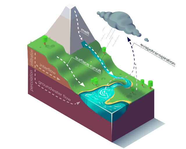
Hydrologic models accept as inputs things like precipitation, solar radiation, soil moisture and the like, and produce a forecast for the river discharge (among other things), days into the future. These models are traditionally implemented using a combination of conceptual models approximating different core processes such as snowmelt, surface runoff, evapotranspiration and more.
The core processes of a hydrologic model. Designed by Daniel Klotz, JKU Institute for Machine Learning.
These models also traditionally require a large amount of manual calibration, and tend to underperform in data scarce regions. We are exploring how multi-task learning can be used to address both of these problems — making hydrologic models both more scalable, and more accurate. In research collaboration with JKU Institute For Machine Learning group under Sepp Hochreiter on developing ML-based hydrologic models, Kratzert et al. show how LSTMs perform better than all benchmarked classic hydrologic models.
The distribution of NSE scores on basins across the United States for various models, showing the proposed EA-LSTM consistently outperforming a wide range of commonly used models.
Though this work is still in the basic research stage and not yet operational, we think it is an important first step, and hope it can already be useful for other researchers and hydrologists. It’s an incredible privilege to take part in the large eco-system of researchers, governments, and NGOs working to reduce the harms of flooding. We’re excited about the potential impact this type of research can provide, and look forward to where research in this field will go.

Acknowledgements
There are many people who contributed to this large effort, and we’d like to highlight some of the key contributors: Aaron Yonas, Adi Mano, Ajai Tirumali, Avinatan Hassidim, Carla Bromberg, Damien Pierce, Gal Elidan, Guy Shalev, John Anderson, Karan Agarwal, Kartik Murthy, Manan Singhi, Mor Schlesinger, Ofir Reich, Oleg Zlydenko, Pete Giencke, Piyush Poddar, Ruha Devanesan, Slava Salasin, Varun Gulshan, Vova Anisimov, Yossi Matias, Yi-fan Chen, Yotam Gigi, Yusef Shafi, Zach Moshe and Zvika Ben-Haim.


Source: Google AI Blog