Author Archives: Google Blogs

Looking to Listen: Audio-Visual Speech Separation


People are remarkably good at focusing their attention on a particular person in a noisy environment, mentally “muting” all other voices and sounds. Known as the cocktail party effect, this capability comes natural to us humans. However, automatic speech separation — separating an audio signal into its individual speech sources — while a well-studied problem, remains a significant challenge for computers.

In “Looking to Listen at the Cocktail Party”, we present a deep learning audio-visual model for isolating a single speech signal from a mixture of sounds such as other voices and background noise. In this work, we are able to computationally produce videos in which speech of specific people is enhanced while all other sounds are suppressed. Our method works on ordinary videos with a single audio track, and all that is required from the user is to select the face of the person in the video they want to hear, or to have such a person be selected algorithmically based on context. We believe this capability can have a wide range of applications, from speech enhancement and recognition in videos, through video conferencing, to improved hearing aids, especially in situations where there are multiple people speaking.
A unique aspect of our technique is in combining both the auditory and visual signals of an input video to separate the speech. Intuitively, movements of a person’s mouth, for example, should correlate with the sounds produced as that person is speaking, which in turn can help identify which parts of the audio correspond to that person. The visual signal not only improves the speech separation quality significantly in cases of mixed speech (compared to speech separation using audio alone, as we demonstrate in our paper), but, importantly, it also associates the separated, clean speech tracks with the visible speakers in the video.
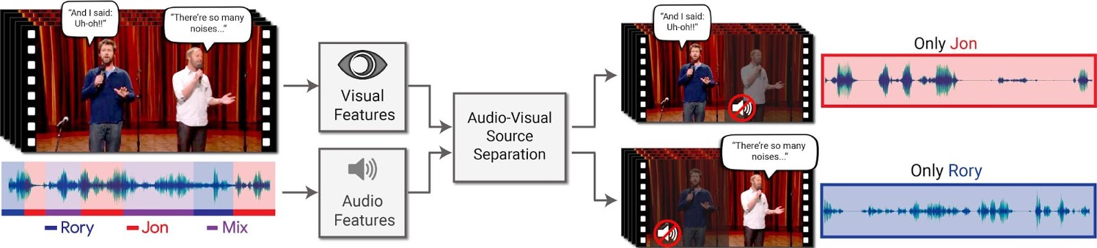
The input to our method is a video with one or more people speaking, where the speech of interest is interfered by other speakers and/or background noise. The output is a decomposition of the input audio track into clean speech tracks, one for each person detected in the video.
An Audio-Visual Speech Separation Model
To generate training examples, we started by gathering a large collection of 100,000 high-quality videos of lectures and talks from YouTube. From these videos, we extracted segments with a clean speech (e.g. no mixed music, audience sounds or other speakers) and with a single speaker visible in the video frames. This resulted in roughly 2000 hours of video clips, each of a single person visible to the camera and talking with no background interference. We then used this clean data to generate “synthetic cocktail parties” -- mixtures of face videos and their corresponding speech from separate video sources, along with non-speech background noise we obtained from AudioSet.

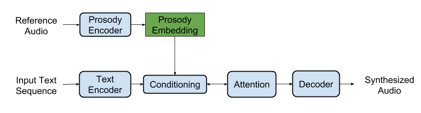
Using this data, we were able to train a multi-stream convolutional neural network-based model to split the synthetic cocktail mixture into separate audio streams for each speaker in the video. The input to the network are visual features extracted from the face thumbnails of detected speakers in each frame, and a spectrogram representation of the video’s soundtrack. During training, the network learns (separate) encodings for the visual and auditory signals, then it fuses them together to form a joint audio-visual representation. With that joint representation, the network learns to output a time-frequency mask for each speaker. The output masks are multiplied by the noisy input spectrogram and converted back to a time-domain waveform to obtain an isolated, clean speech signal for each speaker. For full details, see our paper.
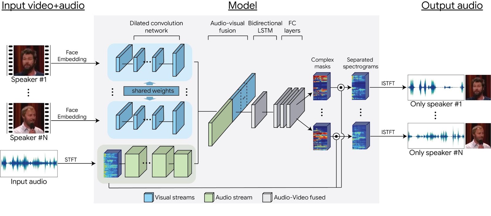
Our multi-stream, neural network-based model architecture.
Here are some more speech separation and enhancement results by our method, playing first the input video with mixed or noisy speech, then our results. Sound by others than the selected speakers can be entirely suppressed or suppressed to the desired level.
Application to Speech Recognition
Our method can also potentially be used as a pre-process for speech recognition and automatic video captioning. Handling overlapping speakers is a known challenge for automatic captioning systems, and separating the audio to the different sources could help in presenting more accurate and easy-to-read captions.
You can similarly see and compare the captions before and after speech separation in all the other videos in this post and on our website, by turning on closed captions in the YouTube player when playing the videos (“cc” button at the lower right corner of the player).

On our project web page you can find more results, as well as comparisons with state-of-the-art audio-only speech separation and with other recent audio-visual speech separation work. Indeed, with recent advances in deep learning, there is a clear growing interest in the academic community in audio-visual analysis. For example, independently and concurrently to our work, this work from UC Berkeley explored a self-supervised approach for separating speech of on/off-screen speakers, and this work from MIT addressed the problem of separating the sound of multiple on-screen objects (e.g., musical instruments), while locating the image regions from which the sound originates.

We envision a wide range of applications for this technology. We are currently exploring opportunities for incorporating it into various Google products. Stay tuned!

Acknowledgements
The research described in this post was done by Ariel Ephrat (as an intern), Inbar Mosseri, Oran Lang, Tali Dekel, Kevin Wilson, Avinatan Hassidim, Bill Freeman and Michael Rubinstein. We would like to thank Yossi Matias and Google Research Israel for their support for the project, and John Hershey for his valuable feedback. We also thank Arkady Ziefman for his help with animations and figures, and Rachel Soh for helping us procure permissions for video content in our results.

Source: Google AI Blog


Announcing the 2018 Google PhD Fellows for North America, Europe and the Middle East


Google created the PhD Fellowship program in 2009 to recognize and support outstanding graduate students doing exceptional research in Computer Science and related disciplines. Now in its ninth year, our fellowship program has supported hundreds of future faculty, industry researchers, innovators and entrepreneurs.

Reflecting our continuing commitment to supporting and building relationships with the academic community, we are excited to announce the 39 recipients from North America, Europe and the Middle East. We offer our sincere congratulations to the 2018 Google PhD Fellows.

Algorithms, Optimizations and Markets
Emmanouil Zampetakis, Massachusetts Institute of Technology
Manuela Fischer, ETH Zurich CS
Thodoris Lykouris, Cornell University
Yuan Deng, Duke University

Computational Neuroscience
Ella Batty, Columbia University
Neha Spenta Wadia, University of California, Berkeley
Reuben Feinman, New York University

Human-Computer Interaction
Gierad Laput, Carnegie Mellon University
Mike Schaekermann, University of Waterloo
Minsuk (Brian) Kahng, Georgia Tech

Machine Learning
Aditi Raghunathan, Stanford University
Lin Chen, Yale University
Qian Yu, University of Southern California
Ravid Shwartz-Ziv, The Hebrew University of Jerusalem
Shuang Liu, University of California, San Diego
Stephen Tu, University of California, Berkeley
Xinchen Yan, University of Michigan, Ann Arbor
Zelda Mariet, Massachusetts Institute of Technology

Mobile Computing
Shilin Zhu, University of California, San Diego

Machine Perception, Speech Technology and Computer Vision
Antoine Miech, INRIA
Arsha Nagrani, University of Oxford (ES)
Joseph Redmon, University of Washington
Raymond Yeh, University of Illinois, Urbana-Champaign
Shanmukha Ramakrishna Vedantam, Georgia Tech

Natural Language Processing
Anne Cocos, University of Pennsylvania
Jonathan Herzig, Tel-Aviv University
Rotem Dror, Technion - Israel Institute of Technology
Yang Liu, The University of Edinburgh
Yoon Kim, Harvard University

Privacy and Security
Aayush Jain, University of California, Los Angeles

Programming Technology and Software Engineering
Gowtham Kaki, Purdue University, West Lafayette
Reyhaneh Jabbarvand, University of California, Irvine
Victor Lanvin, Fondation Sciences Mathématiques de Paris

Quantum Computing
Erika Ye, California Institute of Technology

Structured Data and Database Management
Lingjiao Chen, University of Wisconsin

Systems and Networking
Andrea Lattuada, ETH Zurich CS
Lana Josipović, EPFL CS
Michael Schaarschmidt, University of Cambridge - Computer Laboratory
Rachee Singh, University of Massachusetts, Amherst

Source: Google AI Blog


MobileNetV2: The Next Generation of On-Device Computer Vision Networks


Last year we introduced MobileNetV1, a family of general purpose computer vision neural networks designed with mobile devices in mind to support classification, detection and more. The ability to run deep networks on personal mobile devices improves user experience, offering anytime, anywhere access, with additional benefits for security, privacy, and energy consumption. As new applications emerge allowing users to interact with the real world in real time, so does the need for ever more efficient neural networks.

Today, we are pleased to announce the availability of MobileNetV2 to power the next generation of mobile vision applications. MobileNetV2 is a significant improvement over MobileNetV1 and pushes the state of the art for mobile visual recognition including classification, object detection and semantic segmentation. MobileNetV2 is released as part of TensorFlow-Slim Image Classification Library, or you can start exploring MobileNetV2 right away in Colaboratory. Alternately, you can download the notebook and explore it locally using Jupyter. MobileNetV2 is also available as modules on TF-Hub, and pretrained checkpoints can be found on github.

MobileNetV2 builds upon the ideas from MobileNetV1 [1], using depthwise separable convolution as efficient building blocks. However, V2 introduces two new features to the architecture: 1) linear bottlenecks between the layers, and 2) shortcut connections between the bottlenecks1. The basic structure is shown below.
Overview of MobileNetV2 Architecture. Blue blocks represent composite convolutional building blocks as shown above.
The intuition is that the bottlenecks encode the model’s intermediate inputs and outputs while the inner layer encapsulates the model’s ability to transform from lower-level concepts such as pixels to higher level descriptors such as image categories. Finally, as with traditional residual connections, shortcuts enable faster training and better accuracy. You can learn more about the technical details in our paper, “MobileNet V2: Inverted Residuals and Linear Bottlenecks”.

How does it compare to the first generation of MobileNets?
Overall, the MobileNetV2 models are faster for the same accuracy across the entire latency spectrum. In particular, the new models use 2x fewer operations, need 30% fewer parameters and are about 30-40% faster on a Google Pixel phone than MobileNetV1 models, all while achieving higher accuracy.
MobileNetV2 improves speed (reduced latency) and increased ImageNet Top 1 accuracy
MobileNetV2 is a very effective feature extractor for object detection and segmentation. For example, for detection when paired with the newly introduced SSDLite [2] the new model is about 35% faster with the same accuracy than MobileNetV1. We have open sourced the model under the Tensorflow Object Detection API [4].

Model
Params
Multiply-Adds
mAP
Mobile CPU
MobileNetV1 + SSDLite
5.1M
1.3B
22.2%
270ms
4.3M
0.8B
22.1%
200ms

To enable on-device semantic segmentation, we employ MobileNetV2 as a feature extractor in a reduced form of DeepLabv3 [3], that was announced recently. On the semantic segmentation benchmark, PASCAL VOC 2012, our resulting model attains a similar performance as employing MobileNetV1 as feature extractor, but requires 5.3 times fewer parameters and 5.2 times fewer operations in terms of Multiply-Adds.

Model
Params
Multiply-Adds
mIOU
MobileNetV1 + DeepLabV3
11.15M
14.25B
75.29%
2.11M
2.75B
75.32%

As we have seen MobileNetV2 provides a very efficient mobile-oriented model that can be used as a base for many visual recognition tasks. We hope by sharing it with the broader academic and open-source community we can help to advance research and application development.

Acknowledgements:
We would like to acknowledge our core contributors Menglong Zhu, Andrey Zhmoginov and Liang-Chieh Chen. We also give special thanks to Bo Chen, Dmitry Kalenichenko, Skirmantas Kligys, Mathew Tang, Weijun Wang, Benoit Jacob, George Papandreou, Zhichao Lu, Vivek Rathod, Jonathan Huang, Yukun Zhu, and Hartwig Adam.

References
  1. MobileNets: Efficient Convolutional Neural Networks for Mobile Vision Applications, Howard AG, Zhu M, Chen B, Kalenichenko D, Wang W, Weyand T, Andreetto M, Adam H, arXiv:1704.04861, 2017.
  2. MobileNetV2: Inverted Residuals and Linear Bottlenecks, Sandler M, Howard A, Zhu M, Zhmoginov A, Chen LC. arXiv preprint. arXiv:1801.04381, 2018.
  3. Rethinking Atrous Convolution for Semantic Image Segmentation, Chen LC, Papandreou G, Schroff F, Adam H. arXiv:1706.05587, 2017.
  4. Speed/accuracy trade-offs for modern convolutional object detectors, Huang J, Rathod V, Sun C, Zhu M, Korattikara A, Fathi A, Fischer I, Wojna Z, Song Y, Guadarrama S, Murphy K, CVPR 2017.
  5. Deep Residual Learning for Image Recognition, He, Kaiming, Xiangyu Zhang, Shaoqing Ren, and Jian Sun. arXiv:1512.03385,2015


1 The shortcut (also known as skip) connections, popularized by ResNets[5] are commonly used to connect the non-bottleneck layers. MobilenNetV2 inverts this notion and connects the bottlenecks directly.

Source: Google AI Blog


Investing in France’s AI Ecosystem


Recently, we announced the launch of a new AI research team in our Paris office. And today DeepMind has also announced a new AI research presence in Paris. We are excited about expanding Google’s research presence in Europe, which bolsters the efforts of the existing groups in our Zürich and London offices. As strong supporters of academic research, we are also excited to foster collaborations with France’s vibrant academic ecosystem.

Our research teams in Paris will focus on fundamental AI research, as well as important applications of these ideas to areas such as Health, Science or Arts. They will publish and open-source their results to advance the state-of-the-art in core areas such as Deep Learning and Reinforcement Learning.

Our approach to research is based on building a strong connection with the academic community; contributing to training the next generation of scientists and establishing a bridge between academic and industrial research. We believe that both objectives are key to fostering a healthy research ecosystem that will flourish in the long term. These ideas are very much aligned with some of the recommendations that Fields Medalist and member of French Parliament Cédric Villani is putting forward in his report on AI to the French government.

As we expand our teams in France, we have several initiatives that illustrate our commitment to these goals:
  • We are sponsoring “Artificial Intelligence and Visual Computing” Chair at École Polytechnique (one of the leading higher education institutions in France) which will support their education initiatives in AI
  • We just established a partnership with INRIA for conducting collaborative research projects
  • We are funding academic research with unrestricted grants mostly dedicated to the support of PhD and postdoc positions through our Faculty Research Awards and PhD Fellowship programs, as well as our Focused Research Awards. As one example, we have recently funded a project on large scale optimization of neural networks led by Francis Bach (INRIA and ENS) and Alexandre d’Aspremont (CNRS and ENS)
  • We are working on offering CIFRE PhD positions (joint PhD positions between Google and an academic lab) as well as internships for PhD students
Additionally, we are pleased to announce that one of the world’s leading experts in computer vision, Cordelia Schmid, will begin a dual appointment at INRIA and Google Paris. These kind of appointments, together with our Visiting Faculty program, are a great way to share ideas and research challenges, and utilize Google's world-class computing infrastructure to explore new projects at industrial scale.

France has a long tradition of research and educational excellence, and has a very dynamic and active machine learning community. This makes it a great place to pursue our goal of building AI-enabled technologies that can benefit everyone, through fundamental advances in machine learning and related fields.

Source: Google AI Blog


Using Machine Learning to Discover Neural Network Optimizers


Deep learning models have been deployed in numerous Google products, such as Search, Translate and Photos. The choice of optimization method plays a major role when training deep learning models. For example, stochastic gradient descent works well in many situations, but more advanced optimizers can be faster, especially for training very deep networks. Coming up with new optimizers for neural networks, however, is challenging due to to the non-convex nature of the optimization problem. On the Google Brain team, we wanted to see if it could be possible to automate the discovery of new optimizers, in a way that is similar to how AutoML has been used to discover new competitive neural network architectures.

In “Neural Optimizer Search with Reinforcement Learning”, we present a method to discover optimization methods with a focus on deep learning architectures. Using this method we found two new optimizers, PowerSign and AddSign, that are competitive on a variety of different tasks and architectures, including ImageNet classification and Google’s neural machine translation system. To help others benefit from this work we have made the optimizers available in Tensorflow.

Neural Optimizer Search makes use of a recurrent neural network controller which is given access to a list of simple primitives that are typically relevant for optimization. These primitives include, for example, the gradient or the running average of the gradient and lead to search spaces with over 1010 possible combinations. The controller then generates the computation graph for a candidate optimizer or update rule in that search space.

In our paper, proposed candidate update rules (U) are used to train a child convolutional neural network on CIFAR10 for a few epochs and the final validation accuracy (R) is fed as a reward to the controller. The controller is trained with reinforcement learning to maximize the validation accuracies of the sampled update rules. This process is illustrated below.
An overview of Neural Optimizer Search using an iterative process to discover new optimizers.
Interestingly, the optimizers we have found are interpretable. For example, in the PowerSign optimizer we are releasing, each update compares the sign of the gradient and its running average, adjusting the step size according to whether those two values agree. The intuition behind this is that if these values agree, one is more confident in the direction of the update, and thus the step size can be larger. We also discovered a simple learning rate decay scheme, linear cosine decay, which we found can lead to faster convergence.
Graph comparing learning rate decay functions for linear cosine decay, stepwise decay and cosine decay.
Neural Optimizer Search found several optimizers that outperform commonly used optimizers on the small ConvNet model. Among the ones that transfer well to other tasks, we found that PowerSign and AddSign improve top-1 and top-5 accuracy of a state-of-the-art ImageNet mobile-sized model by up to 0.4%. They also work well on Google’s Neural Machine Translation system, giving an improvement of up to 0.7 using bilingual evaluation metrics (BLEU) on an English to German translation task.

We are excited that Neural Optimizer Search can not only improve the performance of machine learning models but also potentially lead to new, interpretable equations and discoveries. It is our hope that open sourcing these optimizers in Tensorflow will be useful to machine learning practitioners.

Source: Google AI Blog


Expressive Speech Synthesis with Tacotron

At Google, we’re excited about the recent rapid progress of neural network-based text-to-speech (TTS) research. In particular, end-to-end architectures, such as the Tacotron systems we announced last year, can both simplify voice building pipelines and produce natural-sounding speech. This will help us build better human-computer interfaces, like conversational assistants, audiobook narration, news readers, or voice design software. To deliver a truly human-like voice, however, a TTS system must learn to model prosody, the collection of expressive factors of speech, such as intonation, stress, and rhythm. Most current end-to-end systems, including Tacotron, don’t explicitly model prosody, meaning they can’t control exactly how the generated speech should sound. This may lead to monotonous-sounding speech, even when models are trained on very expressive datasets like audiobooks, which often contain character voices with significant variation. Today, we are excited to share two new papers that address these problems.

Our first paper, “Towards End-to-End Prosody Transfer for Expressive Speech Synthesis with Tacotron”, introduces the concept of a prosody embedding. We augment the Tacotron architecture with an additional prosody encoder that computes a low-dimensional embedding from a clip of human speech (the reference audio).

We augment Tacotron with a prosody encoder. The lower half of the image is the original Tacotron sequence-to-sequence model. For technical details, please refer to the paper.

This embedding captures characteristics of the audio that are independent of phonetic information and idiosyncratic speaker traits — these are attributes like stress, intonation, and timing. At inference time, we can use this embedding to perform prosody transfer, generating speech in the voice of a completely different speaker, but exhibiting the prosody of the reference.

Text: *Is* that Utah travel agency?
Reference prosody (Australian)
Synthesized without prosody embedding (American)
Synthesized with prosody embedding (American)

The embedding can also transfer fine time-aligned prosody from one phrase to a slightly different phrase, though this technique works best when the reference and target phrases are similar in length and structure.

Reference Text: For the first time in her life she had been danced tired.
Synthesized Text: For the last time in his life he had been handily embarrassed.
Reference prosody (American)
Synthesized without prosody embedding (American)
Synthesized with prosody embedding (American)

Excitingly, we observe prosody transfer even when the reference audio comes from a speaker whose voice is not in Tacotron’s training data.

Text: I’ve Swallowed a Pollywog.
Reference prosody (Unseen American Speaker)
Synthesized without prosody embedding (British)
Synthesized with prosody embedding (British)

This is a promising result, as it paves the way for voice interaction designers to use their own voice to customize speech synthesis. You can listen to the full set of audio demos for “Towards End-to-End Prosody Transfer for Expressive Speech Synthesis with Tacotron” on this web page.

Despite their ability to transfer prosody with high fidelity, the embeddings from the paper above don’t completely disentangle prosody from the content of a reference audio clip. (This explains why they transfer prosody best to phrases of similar structure and length.) Furthermore, they require a clip of reference audio at inference time. A natural question then arises: can we develop a model of expressive speech that alleviates these problems?

In our second paper, “Style Tokens: Unsupervised Style Modeling, Control and Transfer in End-to-End Speech Synthesis”, we do just that. Building upon the architecture in our first paper, we propose a new unsupervised method for modeling latent “factors” of speech. The key to this model is that, rather than learning fine time-aligned prosodic elements, it learns higher-level speaking style patterns that can be transferred across arbitrarily different phrases.

The model works by adding an extra attention mechanism to Tacotron, forcing it to represent the prosody embedding of any speech clip as the linear combination of a fixed set of basis embeddings. We call these embeddings Global Style Tokens (GSTs), and find that they learn text-independent variations in a speaker’s style (soft, high-pitch, intense, etc.), without the need for explicit style labels.

Model architecture of Global Style Tokens. The prosody embedding is decomposed into “style tokens” to enable unsupervised style control and transfer. For technical details, please refer to the paper.

At inference time, we can select or modify the combination weights for the tokens, allowing us to force Tacotron to use a specific speaking style without needing a reference audio clip. Using GSTs, for example, we can make different sentences of varying lengths sound more “lively”, “angry”, “lamenting”, etc:

Text: United Airlines five six three from Los Angeles to New Orleans has Landed.
Style 1
Style 2
Style 3
Style 4
Style 5

The text-independent nature of GSTs make them ideal for style transfer, which takes a reference audio clip spoken in a specific style and transfers its style to any target phrase we choose. To achieve this, we first run inference to predict the GST combination weights for an utterance whose style we want to imitate. We can then feed those combination weights to the model to synthesize completely different phrases — even those with very different lengths and structure — in the same style.

Finally, our paper shows that Global Style Tokens can model more than just speaking style. When trained on noisy YouTube audio from unlabeled speakers, a GST-enabled Tacotron learns to represent noise sources and distinct speakers as separate tokens. This means that by selecting the GSTs we use in inference, we can synthesize speech free of background noise, or speech in the voice of a specific unlabeled speaker from the dataset. This exciting result provides a path towards highly scalable but robust speech synthesis. You can listen to the full set of demos for “Style Tokens: Unsupervised Style Modeling, Control and Transfer in End-to-End Speech Synthesis” on this web page.

We are excited about the potential applications and opportunities that these two bodies of research enable. In the meantime, there are new important research problems to be addressed. We’d like to extend the techniques of the first paper to support prosody transfer in the natural pitch range of the target speaker. We’d also like to develop techniques to select appropriate prosody or speaking style automatically from context, using, for example, the integration of natural language understanding with TTS. Finally, while our first paper proposes an initial set of objective and subjective metrics for prosody transfer, we’d like to develop these further to help establish generally-accepted methods for prosodic evaluation.

Acknowledgements
These projects were done jointly between multiple Google teams. Contributors include RJ Skerry-Ryan, Yuxuan Wang, Daisy Stanton, Eric Battenberg, Ying Xiao, Joel Shor, Rif A. Saurous, Yu Zhang, Ron J. Weiss, Rob Clark, Fei Ren and Ye Jia.

Reformulating Chemistry for More Efficient Quantum Computation


The first known classical “computer” was the Antikythera mechanism, an analog machine used to simulate the classical mechanics governing dynamics of celestial bodies on an astronomical scale. Similarly, a major ambition of quantum computers is to simulate the quantum mechanics governing dynamics of particles on the atomic scale. These simulations are often classically intractable due to the complex quantum mechanics at play. Of particular interest is the simulation of electrons forming chemical bonds, which give rise to the properties of essentially all molecules, materials and chemical reactions.
Left: The first known computing device, the Antikythera mechanism: a classical machine used to simulate classical mechanics. Right: Google’s 22 Xmon qubit “foxtail” chip arranged in a bilinear array on a wafer, the predecessor to Google’s new Bristlecone quantum processor with 72 qubits, a quantum machine we intend to use to simulate quantum mechanics, among other applications.
Since the launch of the Quantum AI team in 2013, we have been developing practical algorithms for quantum processors. In 2015, we conducted the first quantum chemistry experiment on a superconducting quantum computing device, published in Physical Review X. More recently, our quantum simulation effort experimentally simulated exotic phases of matter and released the first software package for quantum computing chemistry, OpenFermion. Earlier this month, our hardware team announced the new Bristlecone quantum processor with 72 qubits.

Today, we highlight two recent publications with theoretical advances that significantly reduce the cost of these quantum computations. Our results were presented at the Quantum Information Processing and IBM ThinkQ conferences.

The first of these works, “Low-Depth Quantum Simulation of Materials,” published this week in Physical Review X, was a collaboration between researchers at Google, the group of Professor Garnet Chan at Caltech and the QuArC group at Microsoft. Our fundamental advance was to realize that by changing how molecules are represented on quantum computers, we can greatly simplify the quantum circuits required to solve the problem. Specifically, we specially design basis sets so that the equations describing the system energies (i.e. the Hamiltonian) become more straightforward to express for quantum computation.

To do this, we focused on using basis sets related to functions (plane waves) used in classical electronic structure calculations to provide a periodic representation of the physical system. This enables one to go beyond the quantum simulation of single-molecules and instead use quantum computers to model realistic materials. For instance, instead of simulating a single lithium hydride molecule floating in free space, with our approach one can quantum simulate a crystal of lithium hydride, which is how the material appears in nature. With larger quantum computers one could study other important materials problems such as the degradation of battery cathodes, chemical reactions involving heterogeneous catalysts, or the unusual electrical properties of graphene and superconductors.

In “Quantum Simulation of Electronic Structure with Linear Depth and Connectivity,” published last week in Physical Review Letters with the same collaborators and a Google intern from the Aspuru-Guzik group at Harvard, we leverage the structure introduced in the work above to design algorithms for near-term quantum computers with qubits laid out in a linear array. Whereas past methods required such quantum computers to run for time scaling as the fifth power of the number of simulated electrons for each dynamic step, our improved algorithm runs for time scaling linearly with respect to the number of electrons. This reduction in computational cost makes it viable to perform quantum chemistry simulations on near-term devices with fewer gates in each quantum circuit, possibly avoiding the need for full error-correction.

Even with these improvements, it is no small task to deploy such new technology to outperform classical quantum chemistry algorithms and methods which have been refined in parallel with the development of classical computers for more than eighty years. However, at the current rate of advances in quantum algorithms and hardware, quantum technologies may provide chemists with an invaluable new tool. We look forward to sharing our research results as they develop.

Source: Google AI Blog


Google Faculty Research Awards 2017


We’ve just completed another round of the Google Faculty Research Awards, our annual open call for proposals on computer science and related topics such as machine learning, machine perception, natural language processing, and quantum computing. Our grants cover tuition for a graduate student and provide both faculty and students the opportunity to work directly with Google researchers and engineers.

This round we received 1033 proposals covering 46 countries and over 360 universities. After expert reviews and committee discussions, we decided to fund 152 projects. The subject areas that received the most support this year were human computer interaction, machine learning, machine perception, and systems. Here are a few observations from this round:
  • There was a 17% increase in the total number of proposals received
  • There was a 87% increase in the number of proposals from Asia Pacific universities
  • Proposals focused on Computational Neuroscience increased 53%
  • Proposals focused on Quantum Computing more than doubled this round
Congratulations to the well-deserving recipients of this round’s awards. If you are interested in applying for the next round (September 2018 deadline), please visit our website for more information. You can find award recipients from previous years here.

Source: Google AI Blog


Using Deep Learning to Facilitate Scientific Image Analysis


Many scientific imaging applications, especially microscopy, can produce terabytes of data per day. These applications can benefit from recent advances in computer vision and deep learning. In our work with biologists on robotic microscopy applications (e.g., to distinguish cellular phenotypes) we've learned that assembling high quality image datasets that separate signal from noise is a difficult but important task. We've also learned that there are many scientists who may not write code, but who are still excited to utilize deep learning in their image analysis work. A particular challenge we can help address involves dealing with out-of-focus images. Even with the autofocus systems on state-of-the-art microscopes, poor configuration or hardware incompatibility may result in image quality issues. Having an automated way to rate focus quality can enable the detection, troubleshooting and removal of such images.

Deep Learning to the Rescue
In “Assessing Microscope Image Focus Quality with Deep Learning”, we trained a deep neural network to rate the focus quality of microscopy images with higher accuracy than previous methods. We also integrated the pre-trained TensorFlow model with plugins in Fiji (ImageJ) and CellProfiler, two leading open source scientific image analysis tools that can be used with either a graphical user interface or invoked via scripts.
A pre-trained TensorFlow model rates focus quality for a montage of microscope image patches of cells in Fiji (ImageJ). Hue and lightness of the borders denote predicted focus quality and prediction uncertainty, respectively.
Our publication and source code (TensorFlow, Fiji, CellProfiler) illustrate the basics of a machine learning project workflow: assembling a training dataset (we synthetically defocused 384 in-focus images of cells, avoiding the need for a hand-labeled dataset), training a model using data augmentation, evaluating generalization (in our case, on unseen cell types acquired by an additional microscope) and deploying the pre-trained model. Previous tools for identifying image focus quality often require a user to manually review images for each dataset to determine a threshold between in and out-of-focus images; our pre-trained model requires no user set parameters to use, and can rate focus quality more accurately as well. To help improve interpretability, our model evaluates focus quality on 84×84 pixel patches which can be visualized with colored patch borders.

What about Images without Objects?
An interesting challenge we overcame was that there are often "blank" image patches with no objects, a scenario where no notion of focus quality exists. Instead of explicitly labeling these "blank" patches and teaching our model to recognize them as a separate category, we configured our model to predict a probability distribution across defocus levels, allowing it to learn to express uncertainty (dim borders in the figure) for these empty patches (e.g. predict equal probability in/out-of-focus).

What's Next?
Deep learning-based approaches for scientific image analysis will improve accuracy, reduce manual parameter tuning and may reveal new insights. Clearly, the sharing and availability of datasets and models, and implementation into tools that are proven to be useful within respective communities, will be important for widespread adoption.

Acknowledgements
We thank Claire McQuin, Allen Goodman, Anne Carpenter of the Broad Institute and Kevin Eliceiri of the University of Wisconsin at Madison for assistance with CellProfiler and Fiji integration, respectively.

Source: Google AI Blog


Using Evolutionary AutoML to Discover Neural Network Architectures


The brain has evolved over a long time, from very simple worm brains 500 million years ago to a diversity of modern structures today. The human brain, for example, can accomplish a wide variety of activities, many of them effortlessly — telling whether a visual scene contains animals or buildings feels trivial to us, for example. To perform activities like these, artificial neural networks require careful design by experts over years of difficult research, and typically address one specific task, such as to find what's in a photograph, to call a genetic variant, or to help diagnose a disease. Ideally, one would want to have an automated method to generate the right architecture for any given task.

One approach to generate these architectures is through the use of evolutionary algorithms. Traditional research into neuro-evolution of topologies (e.g. Stanley and Miikkulainen 2002) has laid the foundations that allow us to apply these algorithms at scale today, and many groups are working on the subject, including OpenAI, Uber Labs, Sentient Labs and DeepMind. Of course, the Google Brain team has been thinking about AutoML too. In addition to learning-based approaches (eg. reinforcement learning), we wondered if we could use our computational resources to programmatically evolve image classifiers at unprecedented scale. Can we achieve solutions with minimal expert participation? How good can today's artificially-evolved neural networks be? We address these questions through two papers.

In “Large-Scale Evolution of Image Classifiers,” presented at ICML 2017, we set up an evolutionary process with simple building blocks and trivial initial conditions. The idea was to "sit back" and let evolution at scale do the work of constructing the architecture. Starting from very simple networks, the process found classifiers comparable to hand-designed models at the time. This was encouraging because many applications may require little user participation. For example, some users may need a better model but may not have the time to become machine learning experts. A natural question to consider next was whether a combination of hand-design and evolution could do better than either approach alone. Thus, in our more recent paper, “Regularized Evolution for Image Classifier Architecture Search” (2018), we participated in the process by providing sophisticated building blocks and good initial conditions (discussed below). Moreover, we scaled up computation using Google's new TPUv2 chips. This combination of modern hardware, expert knowledge, and evolution worked together to produce state-of-the-art models on CIFAR-10 and ImageNet, two popular benchmarks for image classification.

A Simple Approach
The following is an example of an experiment from our first paper. In the figure below, each dot is a neural network trained on the CIFAR-10 dataset, which is commonly used to train image classifiers. Initially, the population consists of one thousand identical simple seed models (no hidden layers). Starting from simple seed models is important — if we had started from a high-quality model with initial conditions containing expert knowledge, it would have been easier to get a high-quality model in the end. Once seeded with the simple models, the process advances in steps. At each step, a pair of neural networks is chosen at random. The network with higher accuracy is selected as a parent and is copied and mutated to generate a child that is then added to the population, while the other neural network dies out. All other networks remain unchanged during the step. With the application of many such steps in succession, the population evolves.
Progress of an evolution experiment. Each dot represents an individual in the population. The four diagrams show examples of discovered architectures. These correspond to the best individual (rightmost; selected by validation accuracy) and three of its ancestors.
The mutations in our first paper are purposefully simple: remove a convolution at random, add a skip connection between arbitrary layers, or change the learning rate, to name a few. This way, the results show the potential of the evolutionary algorithm, as opposed to the quality of the search space. For example, if we had used a single mutation that transforms one of the seed networks into an Inception-ResNet classifier in one step, we would be incorrectly concluding that the algorithm found a good answer. Yet, in that case, all we would have done is hard-coded the final answer into a complex mutation, rigging the outcome. If instead we stick with simple mutations, this cannot happen and evolution is truly doing the job. In the experiment in the figure, simple mutations and the selection process cause the networks to improve over time and reach high test accuracies, even though the test set had never been seen during the process. In this paper, the networks can also inherit their parent's weights. Thus, in addition to evolving the architecture, the population trains its networks while exploring the search space of initial conditions and learning-rate schedules. As a result, the process yields fully trained models with optimized hyperparameters. No expert input is needed after the experiment starts.

In all the above, even though we were minimizing the researcher's participation by having simple initial architectures and intuitive mutations, a good amount of expert knowledge went into the building blocks those architectures were made of. These included important inventions such as convolutions, ReLUs and batch-normalization layers. We were evolving an architecture made up of these components. The term "architecture" is not accidental: this is analogous to constructing a house with high-quality bricks.

Combining Evolution and Hand Design
After our first paper, we wanted to reduce the search space to something more manageable by giving the algorithm fewer choices to explore. Using our architectural analogy, we removed all the possible ways of making large-scale errors, such as putting the wall above the roof, from the search space. Similarly with neural network architecture searches, by fixing the large-scale structure of the network, we can help the algorithm out. So how to do this? The inception-like modules introduced in Zoph et al. (2017) for the purpose of architecture search proved very powerful. Their idea is to have a deep stack of repeated modules called cells. The stack is fixed but the architecture of the individual modules can change.
The building blocks introduced in Zoph et al. (2017). The diagram on the left is the outer structure of the full neural network, which parses the input data from bottom to top through a stack of repeated cells. The diagram on the right is the inside structure of a cell. The goal is to find a cell that yields an accurate network.
In our second paper, “Regularized Evolution for Image Classifier Architecture Search” (2018), we presented the results of applying evolutionary algorithms to the search space described above. The mutations modify the cell by randomly reconnecting the inputs (the arrows on the right diagram in the figure) or randomly replacing the operations (for example, they can replace the "max 3x3" in the figure, a max-pool operation, with an arbitrary alternative). These mutations are still relatively simple, but the initial conditions are not: the population is now initialized with models that must conform to the outer stack of cells, which was designed by an expert. Even though the cells in these seed models are random, we are no longer starting from simple models, which makes it easier to get to high-quality models in the end. If the evolutionary algorithm is contributing meaningfully, the final networks should be significantly better than the networks we already know can be constructed within this search space. Our paper shows that evolution can indeed find state-of-the-art models that either match or outperform hand-designs.

A Controlled Comparison
Even though the mutation/selection evolutionary process is not complicated, maybe an even more straightforward approach (like random search) could have done the same. Other alternatives, though not simpler, also exist in the literature (like reinforcement learning). Because of this, the main purpose of our second paper was to provide a controlled comparison between techniques.
Comparison between evolution, reinforcement learning, and random search for the purposes of architecture search. These experiments were done on the CIFAR-10 dataset, under the same conditions as Zoph et al. (2017), where the search space was originally used with reinforcement learning.
The figure above compares evolution, reinforcement learning, and random search. On the left, each curve represents the progress of an experiment, showing that evolution is faster than reinforcement learning in the earlier stages of the search. This is significant because with less compute power available, the experiments may have to stop early. Moreover evolution is quite robust to changes in the dataset or search space. Overall, the goal of this controlled comparison is to provide the research community with the results of a computationally expensive experiment. In doing so, it is our hope to facilitate architecture searches for everyone by providing a case study of the relationship between the different search algorithms. Note, for example, that the figure above shows that the final models obtained with evolution can reach very high accuracy while using fewer floating-point operations.

One important feature of the evolutionary algorithm we used in our second paper is a form of regularization: instead of letting the worst neural networks die, we remove the oldest ones — regardless of how good they are. This improves robustness to changes in the task being optimized and tends to produce more accurate networks in the end. One reason for this may be that since we didn't allow weight inheritance, all networks must train from scratch. Therefore, this form of regularization selects for networks that remain good when they are re-trained. In other words, because a model can be more accurate just by chance — noise in the training process means even identical architectures may get different accuracy values — only architectures that remain accurate through the generations will survive in the long run, leading to the selection of networks that retrain well. More details of this conjecture can be found in the paper.

The state-of-the-art models we evolved are nicknamed AmoebaNets, and are one of the latest results from our AutoML efforts. All these experiments took a lot of computation — we used hundreds of GPUs/TPUs for days. Much like a single modern computer can outperform thousands of decades-old machines, we hope that in the future these experiments will become household. Here we aimed to provide a glimpse into that future.

Acknowledgements
We would like to thank Alok Aggarwal, Yanping Huang, Andrew Selle, Sherry Moore, Saurabh Saxena, Yutaka Leon Suematsu, Jie Tan, Alex Kurakin, Quoc Le, Barret Zoph, Jon Shlens, Vijay Vasudevan, Vincent Vanhoucke, Megan Kacholia, Jeff Dean, and the rest of the Google Brain team for the collaborations that made this work possible.

Source: Google AI Blog