Tag Archives: Video Analysis

Scaling multimodal understanding to long videos

When building machine learning models for real-life applications, we need to consider inputs from multiple modalities in order to capture various aspects of the world around us. For example, audio, video, and text all provide varied and complementary information about a visual input. However, building multimodal models is challenging due to the heterogeneity of the modalities. Some of the modalities might be well synchronized in time (e.g., audio, video) but not aligned with text. Furthermore, the large volume of data in video and audio signals is much larger than that in text, so when combining them in multimodal models, video and audio often cannot be fully consumed and need to be disproportionately compressed. This problem is exacerbated for longer video inputs.

In “Mirasol3B: A Multimodal Autoregressive model for time-aligned and contextual modalities”, we introduce a multimodal autoregressive model (Mirasol3B) for learning across audio, video, and text modalities. The main idea is to decouple the multimodal modeling into separate focused autoregressive models, processing the inputs according to the characteristics of the modalities. Our model consists of an autoregressive component for the time-synchronized modalities (audio and video) and a separate autoregressive component for modalities that are not necessarily time-aligned but are still sequential, e.g., text inputs, such as a title or description. Additionally, the time-aligned modalities are partitioned in time where local features can be jointly learned. In this way, audio-video inputs are modeled in time and are allocated comparatively more parameters than prior works. With this approach, we can effortlessly handle much longer videos (e.g., 128-512 frames) compared to other multimodal models. At 3B parameters, Mirasol3B is compact compared to prior Flamingo (80B) and PaLI-X (55B) models. Finally, Mirasol3B outperforms the state-of-the-art approaches on video question answering (video QA), long video QA, and audio-video-text benchmarks.

The Mirasol3B architecture consists of an autoregressive model for the time-aligned modalities (audio and video), which are partitioned in chunks, and a separate autoregressive model for the unaligned context modalities (e.g., text). Joint feature learning is conducted by the Combiner, which learns compact but sufficiently informative features, allowing the processing of long video/audio inputs.

Coordinating time-aligned and contextual modalities

Video, audio and text are diverse modalities with distinct characteristics. For example, video is a spatio-temporal visual signal with 30–100 frames per second, but due to the large volume of data, typically only 32–64 frames per video are consumed by current models. Audio is a one-dimensional temporal signal obtained at much higher frequency than video (e.g., at 16 Hz), whereas text inputs that apply to the whole video, are typically 200–300 word-sequence and serve as a context to the audio-video inputs. To that end, we propose a model consisting of an autoregressive component that fuses and jointly learns the time-aligned signals, which occur at high frequencies and are roughly synchronized, and another autoregressive component for processing non-aligned signals. Learning between the components for the time-aligned and contextual modalities is coordinated via cross-attention mechanisms that allow the two to exchange information while learning in a sequence without having to synchronize them in time.


Time-aligned autoregressive modeling of video and audio

Long videos can convey rich information and activities happening in a sequence. However, present models approach video modeling by extracting all the information at once, without sufficient temporal information. To address this, we apply an autoregressive modeling strategy where we condition jointly learned video and audio representations for one time interval on feature representations from previous time intervals. This preserves temporal information.

The video is first partitioned into smaller video chunks. Each chunk itself can be 4–64 frames. The features corresponding to each chunk are then processed by a learning module, called the Combiner (described below), which generates a joint audio and video feature representation at the current step — this step extracts and compacts the most important information per chunk. Next, we process this joint feature representation with an autoregressive Transformer, which applies attention to the previous feature representation and generates the joint feature representation for the next step. Consequently, the model learns how to represent not only each individual chunk, but also how the chunks relate temporally.

We use an autoregressive modeling of the audio and video inputs, partitioning them in time and learning joint feature representations, which are then autoregressively learned in sequence.

Modeling long videos with a modality combiner

To combine the signals from the video and audio information in each video chunk, we propose a learning module called the Combiner. Video and audio signals are aligned by taking the audio inputs that correspond to a specific video timeframe. We then process video and audio inputs spatio-temporally, extracting information particularly relevant to changes in the inputs (for videos we use sparse video tubes, and for audio we apply the spectrogram representation, both of which are processed by a Vision Transformer). We concatenate and input these features to the Combiner, which is designed to learn a new feature representation capturing both these inputs. To address the challenge of the large volume of data in video and audio signals, another goal of the Combiner is to reduce the dimensionality of the joint video/audio inputs, which is done by selecting a smaller number of output features to be produced. The Combiner can be implemented simply as a causal Transformer, which processes the inputs in the direction of time, i.e., using only inputs of the prior steps or the current one. Alternatively, the Combiner can have a learnable memory, described below.


Combiner styles

A simple version of the Combiner adapts a Transformer architecture. More specifically, all audio and video features from the current chunk (and optionally prior chunks) are input to a Transformer and projected to a lower dimensionality, i.e., a smaller number of features are selected as the output “combined” features. While Transformers are not typically used in this context, we find it effective for reducing the dimensionality of the input features, by selecting the last m outputs of the Transformer, if m is the desired output dimension (shown below). Alternatively, the Combiner can have a memory component. For example, we use the Token Turing Machine (TTM), which supports a differentiable memory unit, accumulating and compressing features from all previous timesteps. Using a fixed memory allows the model to work with a more compact set of features at every step, rather than process all the features from previous steps, which reduces computation.

We use a simple Transformer-based Combiner (left) and a Memory Combiner (right), based on the Token Turing Machine (TTM), which uses memory to compress previous history of features.

Results

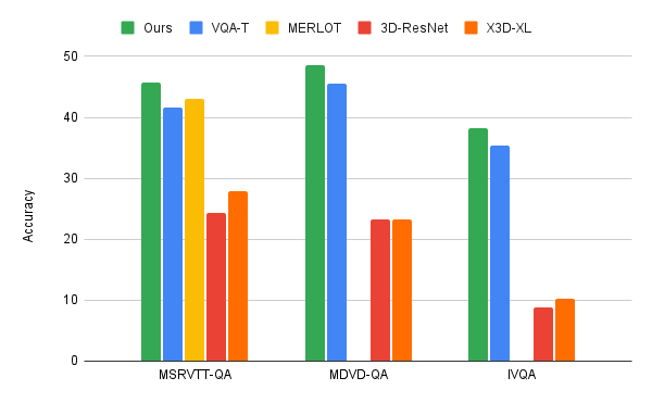
We evaluate our approach on several benchmarks, MSRVTT-QA, ActivityNet-QA and NeXT-QA, for the video QA task, where a text-based question about a video is issued and the model needs to answer. This evaluates the ability of the model to understand both the text-based question and video content, and to form an answer, focusing on only relevant information. Of these benchmarks, the latter two target long video inputs and feature more complex questions.

We also evaluate our approach in the more challenging open-ended text generation setting, wherein the model generates the answers in an unconstrained fashion as free form text, requiring an exact match to the ground truth answer. While this stricter evaluation counts synonyms as incorrect, it may better reflect a model’s ability to generalize.

Our results indicate improved performance over state-of-the-art approaches for most benchmarks, including all with open-ended generation evaluation — notable considering our model is only 3B parameters, considerably smaller than prior approaches, e.g., Flamingo 80B. We used only video and text inputs to be comparable to other work. Importantly, our model can process 512 frames without needing to increase the model parameters, which is crucial for handling longer videos. Finally with the TTM Combiner, we see both better or comparable performance while reducing compute by 18%.

Results on the MSRVTT-QA (video QA) dataset.
Results on NeXT-QA benchmark, which features long videos for the video QA task.

Results on audio-video benchmarks

Results on the popular audio-video datasets VGG-Sound and EPIC-SOUNDS are shown below. Since these benchmarks are classification-only, we treat them as an open-ended text generative setting where our model produces the text of the desired class; e.g., for the class ID corresponding to the “playing drums” activity, we expect the model to generate the text “playing drums”. In some cases our approach outperforms the prior state of the art by large margins, even though our model outputs the results in the generative open-ended setting.

Results on the VGG-Sound (audio-video QA) dataset.
Results on the EPIC-SOUNDS (audio-video QA) dataset.

Benefits of autoregressive modeling

We conduct an ablation study comparing our approach to a set of baselines that use the same input information but with standard methods (i.e., without autoregression and the Combiner). We also compare the effects of pre-training. Because standard methods are ill-suited for processing longer video, this experiment is conducted for 32 frames and four chunks only, across all settings for fair comparison. We see that Mirasol3B’s improvements are still valid for relatively short videos.

Ablation experiments comparing the main components of our model. Using the Combiner, the autoregressive modeling, and pre-training all improve performance.

Conclusion

We present a multimodal autoregressive model that addresses the challenges associated with the heterogeneity of multimodal data by coordinating the learning between time-aligned and time-unaligned modalities. Time-aligned modalities are further processed autoregressively in time with a Combiner, controlling the sequence length and producing powerful representations. We demonstrate that a relatively small model can successfully represent long video and effectively combine with other modalities. We outperform the state-of-the-art approaches (including some much bigger models) on video- and audio-video question answering.


Acknowledgements

This research is co-authored by AJ Piergiovanni, Isaac Noble, Dahun Kim, Michael Ryoo, Victor Gomes, and Anelia Angelova. We thank Claire Cui, Tania Bedrax-Weiss, Abhijit Ogale, Yunhsuan Sung, Ching-Chung Chang, Marvin Ritter, Kristina Toutanova, Ming-Wei Chang, Ashish Thapliyal, Xiyang Luo, Weicheng Kuo, Aren Jansen, Bryan Seybold, Ibrahim Alabdulmohsin, Jialin Wu, Luke Friedman, Trevor Walker, Keerthana Gopalakrishnan, Jason Baldridge, Radu Soricut, Mojtaba Seyedhosseini, Alexander D'Amour, Oliver Wang, Paul Natsev, Tom Duerig, Younghui Wu, Slav Petrov, Zoubin Ghahramani for their help and support. We also thank Tom Small for preparing the animation.

Source: Google AI Blog


Sparse video tubes for joint video and image vision transformers

Video understanding is a challenging problem that requires reasoning about both spatial information (e.g., for objects in a scene, including their locations and relations) and temporal information for activities or events shown in a video. There are many video understanding applications and tasks, such as understanding the semantic content of web videos and robot perception. However, current works, such as ViViT and TimeSFormer, densely process the video and require significant compute, especially as model size plus video length and resolution increase.

In “Rethinking Video ViTs: Sparse Video Tubes for Joint Image and Video Learning”, to be presented at CVPR 2023, we introduce a simple technique that turns a Vision Transformer (ViT) model image encoder into an efficient video backbone using sparse video tubes (learnable visual representations of samples from the video) to reduce the model’s compute needs. This approach can seamlessly process both images and videos, which allows it to leverage both image and video data sources during training. This training further enables our sparse tubes ViT model to coalesce image and video backbones together to serve a dual role as either an image or video backbone (or both), depending on the input. We demonstrate that this model is scalable, can be adapted to large pre-trained ViTs without requiring full fine-tuning, and achieves state-of-the-art results across many video classification benchmarks.

Using sparse video tubes to sample a video, combined with a standard ViT encoder, leads to an efficient visual representation that can be seamlessly shared with image inputs.


Building a joint image-video backbone

Our sparse tube ViT uses a standard ViT backbone, consisting of a stack of Transformer layers, that processes video information. Previous methods, such as ViViT, densely tokenize the video and then apply factorized attention, i.e., the attention weights for each token are computed separately for the temporal and spatial dimensions. In the standard ViT architecture, self-attention is computed over the whole token sequence. When using videos as input, token sequences become quite long, which can make this computation slow. Instead, in the method we propose, the video is sparsely sampled using video tubes, which are 3D learnable visual representations of various shapes and sizes (described in more detail below) from the video. These tubes are used to sparsely sample the video using a large temporal stride, i.e., when a tube kernel is only applied to a few locations in the video, rather than every pixel.

By sparsely sampling the video tubes, we can use the same global self-attention module, rather than factorized attention like ViViT. We experimentally show that the addition of factorized attention layers can harm the performance due to the uninitialized weights. This single stack of transformer layers in the ViT backbone also enables better sharing of the weights and improves performance. Sparse video tube sampling is done by using a large spatial and temporal stride that selects tokens on a fixed grid. The large stride reduces the number of tokens in the full network, while still capturing both spatial and temporal information and enabling the efficient processing of all tokens.


Sparse video tubes

Video tubes are 3D grid-based cuboids that can have different shapes or categories and capture different information with strides and starting locations that can overlap. In the model, we use three distinct tube shapes that capture: (1) only spatial information (resulting in a set of 2D image patches), (2) long temporal information (over a small spatial area), and (3) both spatial and temporal information equally. Tubes that capture only spatial information can be applied to both image and video inputs. Tubes that capture long temporal information or both temporal and spatial information equally are only applied to video inputs. Depending on the input video size, the three tube shapes are applied to the model multiple times to generate tokens.

A fixed position embedding, which captures the global location of each tube (including any strides, offsets, etc.) relative to all the other tubes, is applied to the video tubes. Different from the previous learned position embeddings, this fixed one better enables sparse, overlapping sampling. Capturing the global location of the tube helps the model know where each came from, which is especially helpful when tubes overlap or are sampled from distant video locations. Next, the tube features are concatenated together to form a set of N tokens. These tokens are processed by a standard ViT encoder. Finally, we apply an attention pooling to compress all the tokens into a single representation and input to a fully connected (FC) layer to make the classification (e.g., playing soccer, swimming, etc.).

Our video ViT model works by sampling sparse video tubes from the video (shown at the bottom) to enable either or both image or video inputs to be seamlessly processed. These tubes have different shapes and capture different video features. Tube 1 (yellow) only captures spatial information, resulting in a set of 2D patches that can be applied to image inputs. Tube 2 (red) captures temporal information and some spatial information and tube 3 (green) equally captures both temporal and spatial information (i.e., the spatial size of the tube x and y are the same as the number of frames t). Tubes 2 and 3 can only be applied to video inputs. The position embedding is added to all the tube features.


Scaling video ViTs

The process of building video backbones is computationally intensive, but our sparse tube ViT model enables computationally efficient scaling of video models, leveraging previously trained image backbones. Since image backbones can be adapted to a video backbone, large image backbones can be turned into large video backbones. More specifically, one can transfer the learned video feature representations from a small tube ViT to a large pre-trained image ViT and train the resulting model with video data for only a few steps, as opposed to a full training from scratch.

Our approach enables scaling a sparse tube ViT in a more efficient way. Specifically, the video features from a small video ViT (top network) can be transferred to a large, pre-trained image ViT (bottom network), and further fine-tuned. This requires fewer training steps to achieve strong performance with the large model. This is beneficial as large video models might be prohibitively expensive to train from scratch.


Results

We evaluate our sparse tube ViT approach using Kinetics-400 (shown below), Kinetics-600 and Kinetics-700 datasets and compare its performance to a long list of prior methods. We find that our approach outperforms all prior methods. Importantly, it outperforms all state-of-the-art methods trained jointly on image+video datasets.

Performance compared to several prior works on the popular Kinetics-400 video dataset. Our sparse tube ViT outperforms state-of-the-art methods.

Furthermore, we test our sparse tube ViT model on the Something-Something V2 dataset, which is commonly used to evaluate more dynamic activities, and also report that it outperforms all prior state-of-the-art approaches.

Performance on the Something-Something V2 video dataset.


Visualizing some learned kernels

It is interesting to understand what kind of rudimentary features are being learned by the proposed model. We visualize them below, showing both the 2D patches, which are shared for both images and videos, and video tubes. These visualizations show the 2D or 3D information being captured by the projection layer. For example, in the 2D patches, various common features, like edges and colors, are detected, while the 3D tubes capture basic shapes and how they may change over time.

Visualizations of patches and tubes learned the sparse tube ViT model. Top row are the 2D patches and the remaining two rows are snapshots from the learned video tubes. The tubes show each patch for the 8 or 4 frames to which they are applied.


Conclusions

We have presented a new sparse tube ViT, which can turn a ViT encoder into an efficient video model, and can seamlessly work with both image and video inputs. We also showed that large video encoders can be bootstrapped from small video encoders and image-only ViTs. Our approach outperforms prior methods across several popular video understanding benchmarks. We believe that this simple representation can facilitate much more efficient learning with input videos, seamlessly incorporate either image or video inputs and effectively eliminate the bifurcation of image and video models for future multimodal understanding.


Acknowledgements

This work is conducted by AJ Piergiovanni, Weicheng Kuo and Anelia Angelova, who are now at Google DeepMind. We thank Abhijit Ogale, Luowei Zhou, Claire Cui and our colleagues in Google Research for their helpful discussions, comments, and support.


Source: Google AI Blog


MaMMUT: A simple vision-encoder text-decoder architecture for multimodal tasks

Vision-language foundational models are built on the premise of a single pre-training followed by subsequent adaptation to multiple downstream tasks. Two main and disjoint training scenarios are popular: a CLIP-style contrastive learning and next-token prediction. Contrastive learning trains the model to predict if image-text pairs correctly match, effectively building visual and text representations for the corresponding image and text inputs, whereas next-token prediction predicts the most likely next text token in a sequence, thus learning to generate text, according to the required task. Contrastive learning enables image-text and text-image retrieval tasks, such as finding the image that best matches a certain description, and next-token learning enables text-generative tasks, such as Image Captioning and Visual Question Answering (VQA). While both approaches have demonstrated powerful results, when a model is pre-trained contrastively, it typically does not fare well on text-generative tasks and vice-versa. Furthermore, adaptation to other tasks is often done with complex or inefficient methods. For example, in order to extend a vision-language model to videos, some models need to do inference for each video frame separately. This limits the size of the videos that can be processed to only a few frames and does not fully take advantage of motion information available across frames.

Motivated by this, we present “A Simple Architecture for Joint Learning for MultiModal Tasks”, called MaMMUT, which is able to train jointly for these competing objectives and which provides a foundation for many vision-language tasks either directly or via simple adaptation. MaMMUT is a compact, 2B-parameter multimodal model that trains across contrastive, text generative, and localization-aware objectives. It consists of a single image encoder and a text decoder, which allows for a direct reuse of both components. Furthermore, a straightforward adaptation to video-text tasks requires only using the image encoder once and can handle many more frames than prior work. In line with recent language models (e.g., PaLM, GLaM, GPT3), our architecture uses a decoder-only text model and can be thought of as a simple extension of language models. While modest in size, our model outperforms the state of the art or achieves competitive performance on image-text and text-image retrieval, video question answering (VideoQA), video captioning, open-vocabulary detection, and VQA.

The MaMMUT model enables a wide range of tasks such as image-text/text-image retrieval (top left and top right), VQA (middle left), open-vocabulary detection (middle right), and VideoQA (bottom).

Decoder-only model architecture

One surprising finding is that a single language-decoder is sufficient for all these tasks, which obviates the need for both complex constructs and training procedures presented before. For example, our model (presented to the left in the figure below) consists of a single visual encoder and single text-decoder, connected via cross attention, and trains simultaneously on both contrastive and text-generative types of losses. Comparatively, prior work is either not able to handle image-text retrieval tasks, or applies only some losses to only some parts of the model. To enable multimodal tasks and fully take advantage of the decoder-only model, we need to jointly train both contrastive losses and text-generative captioning-like losses.

MaMMUT architecture (left) is a simple construct consisting of a single vision encoder and a single text decoder. Compared to other popular vision-language models — e.g., PaLI (middle) and ALBEF, CoCa (right) — it trains jointly and efficiently for multiple vision-language tasks, with both contrastive and text-generative losses, fully sharing the weights between the tasks.

Decoder two-pass learning

Decoder-only models for language learning show clear advantages in performance with smaller model size (almost half the parameters). The main challenge for applying them to multimodal settings is to unify the contrastive learning (which uses unconditional sequence-level representation) with captioning (which optimizes the likelihood of a token conditioned on the previous tokens). We propose a two-pass approach to jointly learn these two conflicting types of text representations within the decoder. During the first pass, we utilize cross attention and causal masking to learn the caption generation task — the text features can attend to the image features and predict the tokens in sequence. On the second pass, we disable the cross-attention and causal masking to learn the contrastive task. The text features will not see the image features but can attend bidirectionally to all text tokens at once to produce the final text-based representation. Completing this two-pass approach within the same decoder allows for accommodating both types of tasks that were previously hard to reconcile. While simple, we show that this model architecture is able to provide a foundation for multiple multimodal tasks.

MaMMUT decoder-only two-pass learning enables both contrastive and generative learning paths by the same model.

Another advantage of our architecture is that, since it is trained for these disjoint tasks, it can be seamlessly applied to multiple applications such as image-text and text-image retrieval, VQA, and captioning.

Moreover, MaMMUT easily adapts to video-language tasks. Previous approaches used a vision encoder to process each frame individually, which required applying it multiple times. This is slow and restricts the number of frames the model can handle, typically to only 6–8. With MaMMUT, we use sparse video tubes for lightweight adaptation directly via the spatio-temporal information from the video. Furthermore, adapting the model to Open-Vocabulary Detection is done by simply training to detect bounding-boxes via an object-detection head.

Adaptation of the MaMMUT architecture to video tasks (left) is simple and fully reuses the model. This is done by generating a video “tubes” feature representation, similar to image patches, that are projected to lower dimensional tokens and run through the vision encoder. Unlike prior approaches (right) that need to run multiple individual images through the vision encoder, we use it only once.

Results

Our model achieves excellent zero-shot results on image-text and text-image retrieval without any adaptation, outperforming all previous state-of-the-art models. The results on VQA are competitive with state-of-the-art results, which are achieved by much larger models. The PaLI model (17B parameters) and the Flamingo model (80B) have the best performance on the VQA2.0 dataset, but MaMMUT (2B) has the same accuracy as the 15B PaLI.

MaMMUT outperforms the state of the art (SOTA) on Zero-Shot Image-Text (I2T) and Text-Image (T2I) retrieval on both MS-COCO (top) and Flickr (bottom) benchmarks.
Performance on the VQA2.0 dataset is competitive but does not outperform large models such as Flamingo-80B and PalI-17B. Performance is evaluated in the more challenging open-ended text generation setting.

MaMMUT also outperforms the state-of-the-art on VideoQA, as shown below on the MSRVTT-QA and MSVD-QA datasets. Note that we outperform much bigger models such as Flamingo, which is specifically designed for image+video pre-training and is pre-trained with both image-text and video-text data.

MaMMUT outperforms the SOTA models on VideoQA tasks (MSRVTT-QA dataset, top, MSVD-QA dataset, bottom), outperforming much larger models, e.g., the 5B GIT2 or Flamingo, which uses 80B parameters and is pre-trained for both image-language and vision-language tasks.

Our results outperform the state-of-the-art on open-vocabulary detection fine-tuning as is also shown below.

MAMMUT open-vocabulary detection results on the LVIS dataset compared to state-of-the-art methods. We report the average precisions for rare classes (APr) as is previously adopted in the literature.

Key ingredients

We show that joint training of both contrastive and text-generative objectives is not an easy task, and in our ablations we find that these tasks are served better by different design choices. We see that fewer cross-attention connections are better for retrieval tasks, but more are preferred by VQA tasks. Yet, while this shows that our model’s design choices might be suboptimal for individual tasks, our model is more effective than more complex, or larger, models.

Ablation studies showing that fewer cross-attention connections (1-2) are better for retrieval tasks (top), whereas more connections favor text-generative tasks such as VQA (bottom).

Conclusion

We presented MaMMUT, a simple and compact vision-encoder language-decoder model that jointly trains a number of conflicting objectives to reconcile contrastive-like and text-generative tasks. Our model also serves as a foundation for many more vision-language tasks, achieving state-of-the-art or competitive performance on image-text and text-image retrieval, videoQA, video captioning, open-vocabulary detection and VQA. We hope it can be further used for more multimodal applications.


Acknowledgements

The work described is co-authored by: Weicheng Kuo, AJ Piergiovanni, Dahun Kim, Xiyang Luo, Ben Caine, Wei Li, Abhijit Ogale, Luowei Zhou, Andrew Dai, Zhifeng Chen, Claire Cui, and Anelia Angelova. We would like to thank Mojtaba Seyedhosseini, Vijay Vasudevan, Priya Goyal, Jiahui Yu, Zirui Wang, Yonghui Wu, Runze Li, Jie Mei, Radu Soricut, Qingqing Huang, Andy Ly, Nan Du, Yuxin Wu, Tom Duerig, Paul Natsev, Zoubin Ghahramani for their help and support.

Source: Google AI Blog


Efficient Video-Text Learning with Iterative Co-tokenization

Video is an ubiquitous source of media content that touches on many aspects of people’s day-to-day lives. Increasingly, real-world video applications, such as video captioning, video content analysis, and video question-answering (VideoQA), rely on models that can connect video content with text or natural language. VideoQA is particularly challenging, however, as it requires grasping both semantic information, such as objects in a scene, as well as temporal information, e.g., how things move and interact, both of which must be taken in the context of a natural-language question that holds specific intent. In addition, because videos have many frames, processing all of them to learn spatio-temporal information can be computationally expensive. Nonetheless, understanding all this information enables models to answer complex questions — for example, in the video below, a question about the second ingredient poured in the bowl requires identifying objects (the ingredients), actions (pouring), and temporal ordering (second).

An example input question for the VideoQA task “What is the second ingredient poured into the bowl?” which requires deeper understanding of both the visual and text inputs. The video is an example from the 50 Salads dataset, used under the Creative Commons license.

To address this, in “Video Question Answering with Iterative Video-Text Co-Tokenization”, we introduce a new approach to video-text learning called iterative co-tokenization, which is able to efficiently fuse spatial, temporal and language information for VideoQA. This approach is multi-stream, processing different scale videos with independent backbone models for each to produce video representations that capture different features, e.g., those of high spatial resolution or long temporal durations. The model then applies the co-tokenization module to learn efficient representations from fusing the video streams with the text. This model is highly efficient, using only 67 giga-FLOPs (GFLOPs), which is at least 50% fewer than previous approaches, while giving better performance than alternative state-of-the-art models.

Video-Text Iterative Co-tokenization
The main goal of the model is to produce features from both videos and text (i.e., the user question), jointly allowing their corresponding inputs to interact. A second goal is to do so in an efficient manner, which is highly important for videos since they contain tens to hundreds of frames as input.

The model learns to tokenize the joint video-language inputs into a smaller set of tokens that jointly and efficiently represent both modalities. When tokenizing, we use both modalities to produce a joint compact representation, which is fed to a transformer layer to produce the next level representation. A challenge here, which is also typical in cross-modal learning, is that often the video frame does not correspond directly to the associated text. We address this by adding two learnable linear layers which unify the visual and text feature dimensions before tokenization. This way we enable both video and text to condition how video tokens are learned.

Moreover, a single tokenization step does not allow for further interaction between the two modalities. For that, we use this new feature representation to interact with the video input features and produce another set of tokenized features, which are then fed into the next transformer layer. This iterative process allows the creation of new features, or tokens, which represent a continual refinement of the joint representation from both modalities. At the last step the features are input to a decoder that generates the text output.

As customarily done for VideoQA, we pre-train the model before fine-tuning it on the individual VideoQA datasets. In this work we use the videos automatically annotated with text based on speech recognition, using the HowTo100M dataset instead of pre-training on a large VideoQA dataset. This weaker pre-training data still enables our model to learn video-text features.

Visualization of the video-text iterative co-tokenization approach. Multi-stream video inputs, which are versions of the same video input (e.g., a high resolution, low frame-rate video and a low resolution, high frame-rate video), are efficiently fused together with the text input to produce a text-based answer by the decoder. Instead of processing the inputs directly, the video-text iterative co-tokenization model learns a reduced number of useful tokens from the fused video-language inputs. This process is done iteratively, allowing the current feature tokenization to affect the selection of tokens at the next iteration, thus refining the selection.

Efficient Video Question-Answering
We apply the video-language iterative co-tokenization algorithm to three main VideoQA benchmarks, MSRVTT-QA, MSVD-QA and IVQA, and demonstrate that this approach achieves better results than other state-of-the-art models, while having a modest size. Furthermore, iterative co-tokenization learning yields significant compute savings for video-text learning tasks. The method uses only 67 giga-FLOPs (GFLOPS), which is one sixth the 360 GFLOPS needed when using the popular 3D-ResNet video model jointly with text and is more than twice as efficient as the X3D model. This is all the while producing highly accurate results, outperforming state-of-the-art methods.

Comparison of our iterative co-tokenization approach to previous methods such as MERLOT and VQA-T, as well as, baselines using single ResNet-3D or X3D-XL.

Multi-stream Video Inputs
For VideoQA, or any of a number of other tasks that involve video inputs, we find that multi-stream input is important to more accurately answer questions about both spatial and temporal relationships. Our approach utilizes three video streams at different resolutions and frame-rates: a low-resolution high frame-rate, input video stream (with 32 frames-per-second and spatial resolution 64x64, which we denote as 32x64x64); a high-resolution, low frame-rate video (8x224x224); and one in-between (16x112x112). Despite the apparently more voluminous information to process with three streams, we obtain very efficient models due to the iterative co-tokenization approach. At the same time these additional streams allow extraction of the most pertinent information. For example, as shown in the figure below, questions related to a specific activity in time will produce higher activations in the smaller resolution but high frame-rate video input, whereas questions related to the general activity can be answered from the high resolution input with very few frames. Another benefit of this algorithm is that the tokenization changes depending on the questions asked.

Visualization of the attention maps learned per layer during the video-text co-tokenization. The attention maps differ depending on the question asked for the same video. For example, if the question is related to the general activity (e.g., surfing in the figure above), then the attention maps of the higher resolution low frame-rate inputs are more active and seem to consider more global information. Whereas if the question is more specific, e.g., asking about what happens after an event, the feature maps are more localized and tend to be active in the high frame-rate video input. Furthermore, we see that the low-resolution, high-frame rate video inputs provide more information related to activities in the video.

Conclusion
We present a new approach to video-language learning that focuses on joint learning across video-text modalities. We address the important and challenging task of video question-answering. Our approach is both highly efficient and accurate, outperforming current state-of-the-art models, despite being more efficient. Our approach results in modest model sizes and can gain further improvements with larger models and data. We hope this work provokes more research in vision-language learning to enable more seamless interaction with vision-based media.

Acknowledgements
This work is conducted by AJ Pierviovanni, Kairo Morton, Weicheng Kuo, Michael Ryoo and Anelia Angelova. We thank our collaborators in this research, and Soravit Changpinyo for valuable comments and suggestions, and Claire Cui for suggestions and support. We also thank Tom Small for visualizations.

Source: Google AI Blog


Co-training Transformer with Videos and Images Improves Action Recognition

Action recognition has become a major focus area for the research community because many applications can benefit from improved modeling, such as video retrieval, video captioning, video question-answering, etc. Transformer-based approaches have recently demonstrated state-of-the-art performance on several benchmarks. While Transformer models require data to learn better visual priors compared to ConvNets, action recognition datasets are relatively small in scale. Large Transformer models are typically first trained on image datasets and later fine-tuned on a target action recognition dataset.

While the current pre-training and fine-tuning action recognition paradigm is straightforward and manifests strong empirical results, it may be overly restrictive for building general-purpose action-recognition models. Compared to a dataset like ImageNet that covers a large range of object recognition classes, action recognition datasets like Kinetics and Something-Something-v2 (SSv2) pertain to limited topics. For example, Kinetics include object-centric actions like “cliff diving” and “ice climbing’ while SSv2 contains object-agnostic activities like ’pretending to put something onto something else.’ As a result, we observed poor performance adapting an action recognition model that has been fine-tuned on one dataset to another disparate dataset.

Differences in objects and video backgrounds among datasets further exacerbate learning a general-purpose action recognition classification model. Despite the fact that video datasets may be increasing in size, prior work suggests significant data augmentation and regularization is necessary to achieve strong performance. This latter finding may indicate the model quickly overfits on the target dataset, and as a result, hinders its capacity to generalize to other action recognition tasks.

In “Co-training Transformer with Videos and Images Improves Action Recognition”, we propose a training strategy, named CoVeR, that leverages both image and video data to jointly learn a single general-purpose action recognition model. Our approach is buttressed by two main findings. First, disparate video datasets cover a diverse set of activities, and training them together in a single model could lead to a model that excels at a wide range of activities. Second, video is a perfect source for learning motion information, while images are great for exploiting structural appearance. Leveraging a diverse distribution of image examples may be beneficial in building robust spatial representations in video models. Concretely, CoVeR first pre-trains the model on an image dataset, and during fine-tuning, it simultaneously trains a single model on multiple video and image datasets to build robust spatial and temporal representations for a general-purpose video understanding model.

Architecture and Training Strategy
We applied the CoVeR approach to the recently proposed spatial-temporal video transformer, called TimeSFormer, that contains 24 layers of transformer blocks. Each block contains one temporal attention, one spatial attention, and one multilayer perceptron (MLP) layer. To learn from multiple video and image datasets, we adopt a multi-task learning paradigm and equip the action recognition model with multiple classification heads. We pre-train all non-temporal parameters on the large-scale JFT dataset. During fine-tuning, a batch of videos and images are sampled from multiple video and image datasets. The sampling rate is proportional to the size of the datasets. Each sample within the batch is processed by the TimeSFormer and then distributed to the corresponding classifier to get the predictions.

Compared with the standard training strategy, CoVeR has two advantages. First, as the model is directly trained on multiple datasets, the learned video representations are more general and can be directly evaluated on those datasets without additional fine-tuning. Second, Transformer-based models may easily overfit to a smaller video distribution, thus degrading the generalization of the learned representations. Training on multiple datasets mitigates this challenge by reducing the risk of overfitting.

CoVeR adopts a multi-task learning strategy trained on multiple datasets, each with their own classifier.

Benchmark Results
We evaluate the CoVeR approach to train on Kinetics-400 (K400), Kinetics-600 (K600), Kinetics-700 (K700), SomethingSomething-V2 (SSv2), and Moments-in-Time (MiT) datasets. Compared with other approaches — such as TimeSFormer, Video SwinTransformer, TokenLearner, ViViT, MoViNet, VATT, VidTr, and OmniSource — CoVeR established the new state-of-the-art on multiple datasets (shown below). Unlike previous approaches that train a dedicated model for one single dataset, a model trained by CoVeR can be directly applied to multiple datasets without further fine-tuning.

Model Pretrain Finetune K400 Accuracy
VATT AudioSet+Videos K400 82.1
Omnisource IG-Kinetics-65M K400 83.6
ViViT JFT-300M K400 85.4
Video SwinTrans   ImageNet21K+external   K400 86.8
CoVeR JFT-3B K400+SSv2+MiT+ImNet 87.2
Accuracy comparison on Kinetics-400 (K400) dataset.
Model Pretrain Finetune SSv2 Accuracy
TimeSFormer ImageNet21k SSv2 62.4
VidTr ImageNet21k SSv2 63.0
ViViT ImageNet21k SSv2 65.9
Video SwinTrans   ImageNet21K+external   SSv2 69.6
CoVeR JFT-3B K400+SSv2+MiT+ImNet 70.9
Accuracy comparison on SomethingSomething-V2 (SSv2) dataset.
Model Pretrain Finetune MiT Accuracy
ViViT ImageNet21k MiT 38.5
VidTr ImageNet21k SSv2 41.1
CoVeR JFT-3B K400+SSv2+MiT+ImNet 46.1
Accuracy comparison on Moments-in-Time (MiT) dataset.

Transfer Learning
We use transfer learning to further verify the video action recognition performance and compare with co-training on multiple datasets, results are summarized below. Specifically, we train on the source datasets, then fine-tune and evaluate on the target dataset.

We first consider K400 as the target dataset. CoVeR co-trained on SSv2 and MiT improves the top-1 accuracy on K400→K400 (where the model is trained on K400 and then fine-tuned on K400) by 1.3%, SSv2→K400 by 1.7%, and MiT→K400 by 0.4%. Similarly, we observe that by transferring to SSv2, CoVeR achieves 2%, 1.8%, and 1.1% improvement over SSv2→SSv2, K400→SSv2, and MiT→SSv2, respectively. The 1.2% and 2% performance improvement on K400 and SSv2 indicates that CoVeR co-trained on multiple datasets could learn better visual representations than the standard training paradigm, which is useful for downstream tasks.

Comparison of transfer learning the representation learned by CoVeR and standard training paradigm. A→B means the model is trained on dataset A and then fine-tuned on dataset B.

Conclusion
In this work, we present CoVeR, a training paradigm that jointly learns action recognition and object recognition tasks in a single model for the purpose of constructing a general-purpose action recognition framework. Our analysis indicates that it may be beneficial to integrate many video datasets into one multi-task learning paradigm. We highlight the importance of continuing to learn on image data during fine-tuning to maintain robust spatial representations. Our empirical findings suggest CoVeR can learn a single general-purpose video understanding model which achieves impressive performance across many action recognition datasets without an additional stage of fine-tuning on each downstream application.

Acknowledgements
We would like to thank Christopher Fifty, Wei Han, Andrew M. Dai, Ruoming Pang, and Fei Sha for preparation of the CoVeR paper, Yue Zhao, Hexiang Hu, Zirui Wang, Zitian Chen, Qingqing Huang, Claire Cui and Yonghui Wu for helpful discussions and feedbacks, and others on the Brain Team for support throughout this project.

Source: Google AI Blog


Introducing Omnimattes: A New Approach to Matte Generation using Layered Neural Rendering

Image and video editing operations often rely on accurate mattes — images that define a separation between foreground and background. While recent computer vision techniques can produce high-quality mattes for natural images and videos, allowing real-world applications such as generating synthetic depth-of-field, editing and synthesising images, or removing backgrounds from images, one fundamental piece is missing: the various scene effects that the subject may generate, like shadows, reflections, or smoke, are typically overlooked.

In “Omnimatte: Associating Objects and Their Effects in Video”, presented at CVPR 2021, we describe a new approach to matte generation that leverages layered neural rendering to separate a video into layers called omnimattes that include not only the subjects but also all of the effects related to them in the scene. Whereas a typical state-of-the-art segmentation model extracts masks for the subjects in a scene, for example, a person and a dog, the method proposed here can isolate and extract additional details associated with the subjects, such as shadows cast on the ground.

A state-of-the-art segmentation network (e.g., MaskRCNN) takes an input video (left) and produces plausible masks for people and animals (middle), but misses their associated effects. Our method produces mattes that include not only the subjects, but their shadows as well (right; individual channels for person and dog visualized as blue and green).

Also unlike segmentation masks, omnimattes can capture partially-transparent, soft effects such as reflections, splashes, or tire smoke. Like conventional mattes, omnimattes are RGBA images that can be manipulated using widely-available image or video editing tools, and can be used wherever conventional mattes are used, for example, to insert text into a video underneath a smoke trail.

Layered Decomposition of Video
To generate omnimattes, we split the input video into a set of layers: one for each moving subject, and one additional layer for stationary background objects. In the example below, there is one layer for the person, one for the dog, and one for the background. When merged together using conventional alpha blending, these layers reproduce the input video.

Besides reproducing the video, the decomposition must capture the correct effects in each layer. For example, if the person’s shadow appears in the dog’s layer, the merged layers would still reproduce the input video, but inserting an additional element between the person and dog would produce an obvious error. The challenge is to find a decomposition where each subject’s layer captures only that subject’s effects, producing a true omnimatte.

Our solution is to apply our previously developed layered neural rendering approach to train a convolutional neural network (CNN) to map the subject’s segmentation mask and a background noise image into an omnimatte. Due to their structure, CNNs are naturally inclined to learn correlations between image effects, and the stronger the correlation between the effects, the easier for the CNN to learn. In the above video, for example, the spatial relationships between the person and their shadow, and the dog and its shadow, remain similar as they walk from right to left. The relationships change more (hence, the correlations are weaker) between the person and the dog’s shadow, or the dog and the person’s shadow. The CNN learns the stronger correlations first, leading to the correct decomposition.

The omnimatte system is shown in detail below. In a preprocess, the user chooses the subjects and specifies a layer for each. A segmentation mask for each subject is extracted using an off-the-shelf segmentation network, such as MaskRCNN, and camera transformations relative to the background are found using standard camera stabilization tools. A random noise image is defined in the background reference frame and sampled using the camera transformations to produce per-frame noise images. The noise images provide image features that are random but consistently track the background over time, providing a natural input for the CNN to learn to reconstruct the background colors.

The rendering CNN takes as input the segmentation mask and the per-frame noise images and produces the RGB color images and alpha maps, which capture the transparency of each layer. These outputs are merged using conventional alpha-blending to produce the output frame. The CNN is trained from scratch to reconstruct the input frames by finding and associating the effects not captured in a mask (e.g., shadows, reflections or smoke) with the given foreground layer, and to ensure the subject’s alpha roughly includes the segmentation mask. To make sure the foreground layers only capture the foreground elements and none of the stationary background, a sparsity loss is also applied on the foreground alpha.

A new rendering network is trained for each video. Because the network is only required to reconstruct the single input video, it is able to capture fine structures and fast motion in addition to separating the effects of each subject, as seen below. In the walking example, the omnimatte includes the shadow cast on the slats of the park bench. In the tennis example, the thin shadow and even the tennis ball are captured. In the soccer example, the shadow of the player and the ball are decomposed into their proper layers (with a slight error when the player’s foot is occluded by the ball).

This basic model already works well, but one can improve the results by augmenting the input of the CNN with additional buffers such as optical flow or texture coordinates.

Applications
Once the omnimattes are generated, how can they be used? As shown above, we can remove objects, simply by removing their layer from the composition. We can also duplicate objects, by repeating their layer in the composition. In the example below, the video has been “unwrapped” into a panorama, and the horse duplicated several times to produce a stroboscopic photograph effect. Note that the shadow that the horse casts on the ground and onto the obstacle is correctly captured.

A more subtle, but powerful application is to retime the subjects. Manipulation of time is widely used in film, but usually requires separate shots for each subject and a controlled filming environment. A decomposition into omnimattes makes retiming effects possible for everyday videos using only post-processing, simply by independently changing the playback rate of each layer. Since the omnimattes are standard RGBA images, this retiming edit can be done using conventional video editing software.

The video below is decomposed into three layers, one for each child. The children’s initial, unsynchronized jumps are aligned by simply adjusting the playback rate of their layers, producing realistic retiming for the splashes and reflections in the water.

In the original video (left), each child jumps at a different time. After editing (right), everyone jumps together.

It’s important to consider that any novel technique for manipulating images should be developed and applied responsibly, as it could be misused to produce fake or misleading information. Our technique was developed in accordance with our AI Principles and only allows rearrangement of content already present in the video, but even simple rearrangement can significantly alter the effect of a video, as shown in these examples. Researchers should be aware of these risks.

Future Work
There are a number of exciting directions to improve the quality of the omnimattes. On a practical level, this system currently only supports backgrounds that can be modeled as panoramas, where the position of the camera is fixed. When the camera position moves, the panorama model cannot accurately capture the entire background, and some background elements may clutter the foreground layers (sometimes visible in the above figures). Handling fully general camera motion, such as walking through a room or down a street, would require a 3D background model. Reconstruction of 3D scenes in the presence of moving objects and effects is still a difficult research challenge, but one that has seen promising recent progress.

On a theoretical level, the ability of CNNs to learn correlations is powerful, but still somewhat mysterious, and does not always lead to the expected layer decomposition. While our system allows for manual editing when the automatic result is imperfect, a better solution would be to fully understand the capabilities and limitations of CNNs to learn image correlations. Such an understanding could lead to improved denoising, inpainting, and many other video editing applications besides layer decomposition.

Acknowledgements
Erika Lu, from the University of Oxford, developed the omnimatte system during two internships at Google, in collaboration with Google researchers Forrester Cole, Tali Dekel, Michael Rubinstein, William T. Freeman and David Salesin, and University of Oxford researchers Weidi Xie and Andrew Zisserman.

Thank you to the friends and families of the authors who agreed to appear in the example videos. The “horse jump low”, “lucia”, and “tennis” videos are from the DAVIS 2016 dataset. The soccer video is used by permission from Online Soccer Skills. The car drift video was licensed from Shutterstock.

Source: Google AI Blog


Understanding Contextual Facial Expressions Across the Globe

It might seem reasonable to assume that people’s facial expressions are universal — so, for example, whether a person is from Brazil, India or Canada, their smile upon seeing close friends or their expression of awe at a fireworks display would look essentially the same. But is that really true? Is the association between these facial expressions and their relevant context across geographies indeed universal? What can similarities — or differences — between the situations where someone grins or frowns tell us about how people may be connected across different cultures?

Scientists seeking to answer these questions and to uncover the extent to which people are connected across cultures and geography often use survey-based studies that can rely heavily on local language, norms, and values. However, such studies are not scalable, and often end up with small sample sizes and inconsistent findings.

In contrast to survey-based studies, studying patterns of facial movement provides a more direct understanding of expressive behavior. But analyzing how facial expressions are actually used in everyday life would require researchers to go through millions of hours of real-world footage, which is too time-consuming to do manually. In addition, facial expressions and the contexts in which they are exhibited are complicated, requiring large sample sizes in order to make statistically sound conclusions. While existing studies have produced diverging answers to the question of the universality of facial expressions in given contexts, applying machine learning (ML) in order to appropriately scale the research has the potential to provide clarity.

In “Sixteen facial expressions occur in similar contexts worldwide”, published in Nature, we present research undertaken in collaboration with UC Berkeley to conduct the first large-scale worldwide analysis of how facial expressions are actually used in everyday life, leveraging deep neural networks (DNNs) to drastically scale up expression analysis in a responsible and thoughtful way. Using a dataset of six million publicly available videos across 144 countries, we analyze the contexts in which people use a variety of facial expressions and demonstrate that rich nuances in facial behavior — including subtle expressions — are used in similar social situations around the world.

A Deep Neural Network Measuring Facial Expression
Facial expressions are not static. If one were to examine a person’s expression instant by instant, what might at first appear to be “anger”, may instead end up being “awe”, “surprise” or “confusion”. The interpretation depends on the dynamics of a person’s face as their expression presents itself. The challenge in building a neural network to understand facial expressions, then, is that it must interpret the expression within its temporal context. Training such a system requires a large and diverse, cross-cultural dataset of videos with fully annotated expressions.

To build the dataset, skilled raters manually searched through a broad collection of publicly available videos to identify those likely to contain clips covering all of our pre-selected expression categories. To ensure that the videos matched the region they were assumed to represent, preference in video selection was given to those that included the geographic location of origin. The faces in the videos were then found using a deep convolutional neural network (CNN) — similar to the Google Cloud Face Detection API — that follows faces over the course of the clip using a method based on traditional optical flow. Using an interface similar to Google Crowdsource, annotators then labeled facial expressions across 28 distinct categories if present at any point during the clip. Because the goal was to sample how an average person would perceive an expression, the annotators were not coached or trained, nor were they provided examples or definitions of the target expressions. We discuss additional experiments to evaluate whether the model trained from these annotations was biased below.

Raters were presented videos with a single face highlighted for their attention. They observed the subject throughout the duration of the clip and annotated the facial expressions they exhibited. (source video)

The face detection algorithm established a sequence of locations of each face throughout the video. We then used a pre-trained Inception network to extract features representing the most salient aspects of facial expressions from the faces. The features were then fed into a long short-term memory (LSTM) network, a type of recurrent neural network that is able to model how a facial expression might evolve over time due to its ability to remember salient information from the past.

In order to ensure that the model was making consistent predictions across a range of demographic groups, we evaluated the model fairness on an existing dataset that was constructed using similar facial expression labels, targeting a subset of 16 expressions on which it exhibited the best performance.

The model's performance was consistent across all of the demographic groups represented in the evaluation dataset, which provides supporting evidence that the model trained to annotated facial expressions is not measurably biased. The model’s annotations of those 16 facial expressions across 1,500 images can be explored here.

We modeled the selected face in each video by using a CNN to extract features from the face at each frame, which were then fed into an LSTM network to model the changes in the expression over time. (source video)

Measuring the Contexts Captured in Videos
To understand the context of facial expressions across millions of videos, we used DNNs that could capture the fine-grained content and automatically recognize the context. The first DNN modeled a combination of text features (title and description) associated with a video along with the actual visual content (video-topic model). In addition, we used a DNN that only relied on text features without any visual information (text-topic model). These models predict thousands of labels describing the videos. In our experiments these models were able to identify hundreds of unique contexts (e.g., wedding, sporting event, or fireworks) showcasing the diversity of the data we used for the analysis.

The Covariation Between Expressions and Contexts Around the World
In our first experiment, we analyzed 3 million public videos captured on mobile phones. We chose to focus on mobile uploads because they are more likely to contain natural expressions. We correlated the facial expressions that occurred in the videos to the context annotations derived from the video-topic model. We found 16 kinds of facial expressions had distinct associations with everyday social contexts that were consistent across the world. For instance, the expressions that people associate with amusement occurred more often in videos with practical jokes; expressions that people associate with awe, in videos with fireworks; and triumph, with sporting events. These results have strong implications for discussions about the relative importance of psychologically relevant context in facial expression, compared to other factors, such as those unique to an individual, culture, or society.

Our second experiment analyzed a separate set of 3 million videos, but this time we annotated the contexts with the text-topic model. The results verified that the findings in the first experiment were not driven by subtle influences of facial expressions in the video on the annotations of the video-topic model. In other words we used this experiment to verify our conclusions from the first experiment given the possibility that the video-topic model could implicitly be factoring in facial expressions when computing its content labels.

We correlated the expression and context annotations across all of the videos within each region. Each expression was found to have specific associations with different contexts that were preserved across 12 world regions. For example, here, in red, we can see that expressions people associate with awe were found more often in the context of fireworks, pets, and toys than in other contexts.

In both experiments, the correlations between expressions and contexts appeared to be well-preserved across cultures. To quantify exactly how similar the associations between expressions and contexts were across the 12 different world regions we studied, we computed second-order correlations between each pair of regions. These correlations identify the relationships between different expressions and contexts in each region and then compare them with other regions. We found that 70% of the context–expression associations found in each region are shared across the modern world.

Finally, we asked how many of the 16 kinds of facial expression we measured had distinct associations with different contexts that were preserved around the world. To do so, we applied a method called canonical correlations analysis, which showed that all 16 facial expressions had distinct associations that were preserved across the world.

Conclusions
We were able to examine the contexts in which facial expressions occur in everyday life across cultures at an unprecedented scale. Machine learning allowed us to analyze millions of videos across the world and discover evidence supporting hypotheses that facial expressions are preserved to a degree in similar contexts across cultures.

Our results also leave room for cultural differences. Although the correlations between facial expressions and contexts were 70% consistent around the world, they were up to 30% variable across regions. Neighboring world regions generally had more similar associations between facial expressions and contexts than distant world regions, indicating that the geographic spread of human culture may also play a role in the meanings of facial expressions.

This work shows that we can use machine learning to better understand ourselves and identify common communication elements across cultures. Tools such as DNNs give us the opportunity to provide vast amounts of diverse data in service of scientific discovery, enabling more confidence in the statistical conclusions. We hope our work provides a template for using the tools of machine learning in a responsible way and sparks more innovative research in other scientific domains.

Acknowledgements
Special thanks to our co-authors Dacher Keltner from UC Berkeley, along with Florian Schroff, Brendan Jou, and Hartwig Adam from Google Research. We are also grateful for additional support at Google provided by Laura Rapin, Reena Jana, Will Carter, Unni Nair, Christine Robson, Jen Gennai, Sourish Chaudhuri, Greg Corrado, Brian Eoff, Andrew Smart, Raine Serrano, Blaise Aguera y Arcas, Jay Yagnik, and Carson Mcneil.

Source: Google AI Blog


Using Machine Learning to Detect Deficient Coverage in Colonoscopy Screenings

Colorectal cancer (CRC) is a global health problem and the second deadliest cancer in the United States, resulting in an estimated 900K deaths per year. While deadly, CRC can be prevented by removing small precancerous lesions in the colon, called polyps, before they become cancerous. In fact, it is estimated that a 1% increase in the adenoma detection rate (ADR, defined as the fraction of procedures in which a physician discovers at least one polyp) can lead to a 6% decrease in the rate of interval CRCs (a CRC that is diagnosed within 60 months of a negative colonoscopy).

Colonoscopy is considered the gold standard procedure for the detection and removal of polyps. Unfortunately, the literature indicates that endoscopists miss on average 22%-28% of polyps during colonoscopies; furthermore, 20% to 24% of polyps that have the potential to become cancerous (adenomas) are missed. Two major factors that may cause an endoscopist to miss a polyp are (1) the polyp appears in the field of view, but the endoscopist misses it, perhaps due to its small size or flat shape; and (2) the polyp does not appear in the field of view, as the endoscopist has not fully covered the relevant area during the procedure.

In “Detecting Deficient Coverage in Colonoscopies”, we introduce the Colonoscopy Coverage Deficiency via Depth algorithm, or C2D2, a machine learning-based approach to improving colonoscopy coverage. The C2D2 algorithm performs a local 3D reconstruction of the colon as images are captured during the procedure, and on that basis, identifies which areas of the colon were covered and which remained outside of the field of view. C2D2 can then indicate in real time whether a particular area of the colon has suffered from deficient coverage so the endoscopist can return to that area. Our work proposes a novel approach to compute coverage in real time, for which 3D reconstruction is done using a calibration-free, unsupervised learning method, and evaluate it in a large scale way.

The C2D2 Algorithm
When considering colon coverage, it is important to estimate the coverage fraction — what percentage of the relevant regions were covered by a complete procedure. While a retrospective analysis is useful for the physician and could provide general guidance for future procedures, it is more useful to have real-time estimation of coverage fraction, on a segment by segment basis, i.e. knowledge of what fraction of the current segment has been covered while traversing the colon. The helpfulness of such functionality is clear: during the procedure itself, a physician may be alerted to segments with deficient coverage, and can immediately return to review these areas. Higher coverage will result in a higher proportion of polyps being seen.

The C2D2 algorithm is designed to compute such a segment-by-segment coverage in two phases: computing depth maps for each frame of the colonoscopy video, followed by computation of coverage based on these depth maps.

C2D2 computes a depth image from a single RGB image. Then, based on the computed depth images for a video sequence, C2D2 calculates local coverage, so it can detect where the coverage has been deficient and a second look is required.

Depth map creation consists of both depth estimation as well as pose estimation — the localization of where the endoscope is in space, as well as the direction it is pointing. In addition to the detection of deficient coverage, depth and pose estimation are useful for a variety of other interesting tasks. For example, depth can be used for improved detection of flat polyps, while pose estimation can be used for relocalizing areas of the colon (including polyps) that the endoscopist wishes to revisit, and both together can be used for visualization and navigation.

Top row: RGB image, from which the depth is computed. Bottom row: Depth image as computed by C2D2. Yellow is deeper, blue is shallower. Note that the “tunnel” structure is captured, as well as the Haustral ridges.

In order to compute coverage fractions from these depth maps, we trained C2D2 on two sources of data: synthetic sequences and real sequences. We generated the synthetic videos using a graphical model of a colon. For each synthetic video, ground truth coverage is available in the form of a number between 0 (completely uncovered) and 1 (completely covered). For real sequences, we analyzed de-identified colonoscopy videos, for which ground truth coverage is unavailable.

Performance on Synthetic Videos
When using synthetic videos, the availability of ground truth coverage enables the direct measurement of C2D2’s performance. We quantify this using the mean absolute error (MAE), which indicates how much the algorithm’s prediction differs, on average, from the ground truth. We find that C2D2’s MAE = 0.075; meaning that, on average, the prediction of C2D2 is within 7.5% of the ground truth. By contrast, a group of physicians given the same task achieved MAE = 0.177, i.e., within 17.7% of the ground truth. Thus, the C2D2 attained an accuracy rate 2.4 times higher on synthetic sequences.

Performance on Real Videos
Of course, what matters most is performance on videos of real colonoscopies. The challenge in this case is the absence of ground truth labelling: we don’t know what the actual coverage is. Additionally, one cannot use labels provided by experts directly as they are not always accurate, due to the challenges described earlier. However, C2D2 can still perform inference on real colonoscopy videos. Indeed, the learning pipeline is designed to perform equally well on synthetic and real colonoscopy videos.

To verify performance on real sequences, we used a variant of a technique common in the generative modelling literature, which involves providing video sequences to human experts along with C2D2’s coverage scores for those sequences. We then ask the experts to assess whether C2D2’s score is correct. The idea is that while it is difficult for experts to assign a score directly, the task of verifying a given score is considerably easier. (This is similar to the fact that verifying a proposed solution to an algorithmic problem is generally much easier than computing that solution.) Using this methodology, experts verified C2D2’s score 93% of the time. And in a more qualitative sense, C2D2’s output seems to pass the “eyeball test”, see the figure below.

Coverage on real colonoscopy sequences. Top row: Frames from a well covered sequence — the entire “tunnel” down the lumen may be seen; C2D2 coverage = 0.931. Middle row: A partially covered sequence — the bottom may be seen, but the top is not as visible; C2D2 coverage = 0.427. Bottom row: A poorly covered sequence, much of what is seen is the wall; C2D2 coverage = 0.227.

Next steps
By alerting physicians to missed regions of the colon wall, C2D2 promises to lead to the discovery of more adenomas, thereby increasing the ADR and concomitantly decreasing the rate of interval CRC. This would be of tremendous benefit to patients.

In addition to this work that addresses colonoscopy coverage, we are concurrently conducting research to improve polyp detection by combining C2D2 with an automatic, real-time polyp detection algorithm. This study adds to the mounting evidence that physicians may use machine learning methods to augment their efforts, especially during procedures, to improve the quality of care for patients.

Acknowledgements
This research was conducted by Daniel Freedman, Yochai Blau, Liran Katzir, Amit Aides, Ilan Shimshoni, Danny Veikherman, Tomer Golany, Ariel Gordon, Greg Corrado, Yossi Matias, and Ehud Rivlin, with support from Verily. We would like to thank all of our team members and collaborators who worked on this project with us, including: Nadav Rabani, Chen Barshai, Nia Stoykova, David Ben-Shimol, Jesse Lachter, and Ori Segol, 3D-Systems and many others. We'd also like to thank Yossi Matias for support and guidance. The research was conducted by teams from Google Health and Google Research, Israel.

Source: Google AI Blog


AutoFlip: An Open Source Framework for Intelligent Video Reframing


Videos filmed and edited for television and desktop are typically created and viewed in landscape aspect ratios (16:9 or 4:3). However, with an increasing number of users creating and consuming content on mobile devices, historical aspect ratios don’t always fit the display being used for viewing. Traditional approaches for reframing video to different aspect ratios usually involve static cropping, i.e., specifying a camera viewport, then cropping visual contents that are outside. Unfortunately, these static cropping approaches often lead to unsatisfactory results due to the variety of composition and camera motion styles. More bespoke approaches, however, typically require video curators to manually identify salient contents on each frame, track their transitions from frame-to-frame, and adjust crop regions accordingly throughout the video. This process is often tedious, time-consuming, and error-prone.

To address this problem, we are happy to announce AutoFlip, an open source framework for intelligent video reframing. AutoFlip is built on top of the MediaPipe framework that enables the development of pipelines for processing time-series multimodal data. Taking a video (casually shot or professionally edited) and a target dimension (landscape, square, portrait, etc.) as inputs, AutoFlip analyzes the video content, develops optimal tracking and cropping strategies, and produces an output video with the same duration in the desired aspect ratio.
Left: Original video (16:9). Middle: Reframed using a standard central crop (9:16). Right: Reframed with AutoFlip (9:16). By detecting the subjects of interest, AutoFlip is able to avoid cropping off important visual content.
AutoFlip Overview
AutoFlip provides a fully automatic solution to smart video reframing, making use of state-of-the-art ML-enabled object detection and tracking technologies to intelligently understand video content. AutoFlip detects changes in the composition that signify scene changes in order to isolate scenes for processing. Within each shot, video analysis is used to identify salient content before the scene is reframed by selecting a camera mode and path optimized for the contents.
Shot (Scene) Detection
A scene or shot is a continuous sequence of video without cuts (or jumps). To detect the occurrence of a shot change, AutoFlip computes the color histogram of each frame and compares this with prior frames. If the distribution of frame colors changes at a different rate than a sliding historical window, a shot change is signaled. AutoFlip buffers the video until the scene is complete before making reframing decisions, in order to optimize the reframing for the entire scene.

Video Content Analysis
We utilize deep learning-based object detection models to find interesting, salient content in the frame. This content typically includes people and animals, but other elements may be identified, depending on the application, including text overlays and logos for commercials, or motion and ball detection for sports.

The face and object detection models are integrated into AutoFlip through MediaPipe, which uses TensorFlow Lite on CPU. This structure allows AutoFlip to be extensible, so developers may conveniently add new detection algorithms for different use cases and video content. Each object type is associated with a weight value, which defines its relative importance — the higher the weight, the more influence the feature will have when computing the camera path.
Left: People detection on sports footage. Right: Two face boxes (‘core’ and ‘all’ face landmarks). In narrow portrait crop cases, often only the core landmark box can fit.
Reframing
After identifying the subjects of interest on each frame, logical decisions about how to reframe the content for a new view can be made. AutoFlip automatically chooses an optimal reframing strategy — stationary, panning or tracking — depending on the way objects behave during the scene (e.g., moving around or stationary). In stationary mode, the reframed camera viewport is fixed in a position where important content can be viewed throughout the majority of the scene. This mode can effectively mimic professional cinematography in which a camera is mounted on a stationary tripod or where post-processing stabilization is applied. In other cases, it is best to pan the camera, moving the viewport at a constant velocity. The tracking mode provides continuous and steady tracking of interesting objects as they move around within the frame.

Based on which of these three reframing strategies the algorithm selects, AutoFlip then determines an optimal cropping window for each frame, while best preserving the content of interest. While the bounding boxes track the objects of focus in the scene, they typically exhibit considerable jitter from frame-to-frame and, consequently, are not sufficient to define the cropping window. Instead, we adjust the viewport on each frame through the process of Euclidean-norm optimization, in which we minimize the residuals between a smooth (low-degree polynomial) camera path and the bounding boxes.
Top: Camera paths resulting from following the bounding boxes from frame-to-frame. Bottom: Final smoothed camera paths generated using Euclidean-norm path formation. Left: Scene in which objects are moving around, requiring a tracking camera path. Right: Scene where objects stay close to the same position; a stationary camera covers the content for the full duration of the scene.
AutoFlip’s configuration graph provides settings for either best-effort or required reframing. If it becomes infeasible to cover all the required regions (for example, when they are too spread out on the frame), the pipeline will automatically switch to a less aggressive strategy by applying a letterbox effect, padding the image to fill the frame. For cases where the background is detected as being a solid color, this color is used to create seamless padding; otherwise a blurred version of the original frame is used.
AutoFlip Use Cases
We are excited to release this tool directly to developers and filmmakers, reducing the barriers to their design creativity and reach through the automation of video editing. The ability to adapt any video format to various aspect ratios is becoming increasingly important as the diversity of devices for video content consumption continues to rapidly increase. Whether your use case is portrait to landscape, landscape to portrait, or even small adjustments like 4:3 to 16:9, AutoFlip provides a solution for intelligent, automated and adaptive video reframing.
What’s Next?
Like any machine learning algorithm, AutoFlip can benefit from an improved ability to detect objects relevant to the intent of the video, such as speaker detection for interviews or animated face detection on cartoons. Additionally, a common issue arises when input video has important overlays on the edges of the screen (such as text or logos) as they will often be cropped from the view. By combining text/logo detection and image inpainting technology, we hope that future versions of AutoFlip can reposition foreground objects to better fit the new aspect ratios. Lastly, in situations where padding is required, deep uncrop technology could provide improved ability to expand beyond the original viewable area.

While we work to improve AutoFlip internally at Google, we encourage contributions from developers and filmmakers in the open source communities.

Acknowledgments
We would like to thank our colleagues who contributed to Autoflip, Alexander Panagopoulos, Jenny Jin, Brian Mulford, Yuan Zhang, Alex Chen, Xue Yang, Mickey Wang, Justin Parra, Hartwig Adam, Jingbin Wang, and Weilong Yang; MediaPipe team who helped with open sourcing, Jiuqiang Tang, Tyler Mullen, Mogan Shieh, Ming Guang Yong, and Chuo-Ling Chang.

Source: Google AI Blog