Tag Archives: Machine Perception

Look and Talk: Natural Conversations with Google Assistant

In natural conversations, we don't say people's names every time we speak to each other. Instead, we rely on contextual signaling mechanisms to initiate conversations, and eye contact is often all it takes. Google Assistant, now available in more than 95 countries and over 29 languages, has primarily relied on a hotword mechanism ("Hey Google" or “OK Google”) to help more than 700 million people every month get things done across Assistant devices. As virtual assistants become an integral part of our everyday lives, we're developing ways to initiate conversations more naturally.

At Google I/O 2022, we announced Look and Talk, a major development in our journey to create natural and intuitive ways to interact with Google Assistant-powered home devices. This is the first multimodal, on-device Assistant feature that simultaneously analyzes audio, video, and text to determine when you are speaking to your Nest Hub Max. Using eight machine learning models together, the algorithm can differentiate intentional interactions from passing glances in order to accurately identify a user's intent to engage with Assistant. Once within 5ft of the device, the user may simply look at the screen and talk to start interacting with the Assistant.

We developed Look and Talk in alignment with our AI Principles. It meets our strict audio and video processing requirements, and like our other camera sensing features, video never leaves the device. You can always stop, review and delete your Assistant activity at myactivity.google.com. These added layers of protection enable Look and Talk to work just for those who turn it on, while keeping your data safe.

Google Assistant relies on a number of signals to accurately determine when the user is speaking to it. On the right is a list of signals used with indicators showing when each signal is triggered based on the user's proximity to the device and gaze direction.

Modeling Challenges
The journey of this feature began as a technical prototype built on top of models developed for academic research. Deployment at scale, however, required solving real-world challenges unique to this feature. It had to:

  1. Support a range of demographic characteristics (e.g., age, skin tones).
  2. Adapt to the ambient diversity of the real world, including challenging lighting (e.g., backlighting, shadow patterns) and acoustic conditions (e.g., reverberation, background noise).
  3. Deal with unusual camera perspectives, since smart displays are commonly used as countertop devices and look up at the user(s), unlike the frontal faces typically used in research datasets to train models.
  4. Run in real-time to ensure timely responses while processing video on-device.

The evolution of the algorithm involved experiments with approaches ranging from domain adaptation and personalization to domain-specific dataset development, field-testing and feedback, and repeated tuning of the overall algorithm.

Technology Overview
A Look and Talk interaction has three phases. In the first phase, Assistant uses visual signals to detect when a user is demonstrating an intent to engage with it and then “wakes up” to listen to their utterance. The second phase is designed to further validate and understand the user’s intent using visual and acoustic signals. If any signal in the first or second processing phases indicates that it isn't an Assistant query, Assistant returns to standby mode. These two phases are the core Look and Talk functionality, and are discussed below. The third phase of query fulfillment is typical query flow, and is beyond the scope of this blog.

Phase One: Engaging with Assistant
The first phase of Look and Talk is designed to assess whether an enrolled user is intentionally engaging with Assistant. Look and Talk uses face detection to identify the user’s presence, filters for proximity using the detected face box size to infer distance, and then uses the existing Face Match system to determine whether they are enrolled Look and Talk users.

For an enrolled user within range, an custom eye gaze model determines whether they are looking at the device. This model estimates both the gaze angle and a binary gaze-on-camera confidence from image frames using a multi-tower convolutional neural network architecture, with one tower processing the whole face and another processing patches around the eyes. Since the device screen covers a region underneath the camera that would be natural for a user to look at, we map the gaze angle and binary gaze-on-camera prediction to the device screen area. To ensure that the final prediction is resilient to spurious individual predictions and involuntary eye blinks and saccades, we apply a smoothing function to the individual frame-based predictions to remove spurious individual predictions.

Eye-gaze prediction and post-processing overview.

We enforce stricter attention requirements before informing users that the system is ready for interaction to minimize false triggers, e.g., when a passing user briefly glances at the device. Once the user looking at the device starts speaking, we relax the attention requirement, allowing the user to naturally shift their gaze.

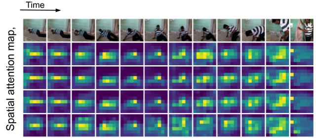
The final signal necessary in this processing phase checks that the Face Matched user is the active speaker. This is provided by a multimodal active speaker detection model that takes as input both video of the user’s face and the audio containing speech, and predicts whether they are speaking. A number of augmentation techniques (including RandAugment, SpecAugment, and augmenting with AudioSet sounds) helps improve prediction quality for the in-home domain, boosting end-feature performance by over 10%.The final deployed model is a quantized, hardware-accelerated TFLite model, which uses five frames of context for the visual input and 0.5 seconds for the audio input.

Active speaker detection model overview: The two-tower audiovisual model provides the “speaking” probability prediction for the face. The visual network auxiliary prediction pushes the visual network to be as good as possible on its own, improving the final multimodal prediction.

Phase Two: Assistant Starts Listening
In phase two, the system starts listening to the content of the user’s query, still entirely on-device, to further assess whether the interaction is intended for Assistant using additional signals. First, Look and Talk uses Voice Match to further ensure that the speaker is enrolled and matches the earlier Face Match signal. Then, it runs a state-of-the-art automatic speech recognition model on-device to transcribe the utterance.

The next critical processing step is the intent understanding algorithm, which predicts whether the user’s utterance was intended to be an Assistant query. This has two parts: 1) a model that analyzes the non-lexical information in the audio (i.e., pitch, speed, hesitation sounds) to determine whether the utterance sounds like an Assistant query, and 2) a text analysis model that determines whether the transcript is an Assistant request. Together, these filter out queries not intended for Assistant. It also uses contextual visual signals to determine the likelihood that the interaction was intended for Assistant.

Overview of the semantic filtering approach to determine if a user utterance is a query intended for the Assistant.

Finally, when the intent understanding model determines that the user utterance was likely meant for Assistant, Look and Talk moves into the fulfillment phase where it communicates with the Assistant server to obtain a response to the user’s intent and query text.

Performance, Personalization and UX
Each model that supports Look and Talk was evaluated and improved in isolation and then tested in the end-to-end Look and Talk system. The huge variety of ambient conditions in which Look and Talk operates necessitates the introduction of personalization parameters for algorithm robustness. By using signals obtained during the user’s hotword-based interactions, the system personalizes parameters to individual users to deliver improvements over the generalized global model. This personalization also runs entirely on-device.

Without a predefined hotword as a proxy for user intent, latency was a significant concern for Look and Talk. Often, a strong enough interaction signal does not occur until well after the user has started speaking, which can add hundreds of milliseconds of latency, and existing models for intent understanding add to this since they require complete, not partial, queries. To bridge this gap, Look and Talk completely forgoes streaming audio to the server, with transcription and intent understanding being on-device. The intent understanding models can work off of partial utterances. This results in an end-to-end latency comparable with current hotword-based systems.

The UI experience is based on user research to provide well-balanced visual feedback with high learnability. This is illustrated in the figure below.

Left: The spatial interaction diagram of a user engaging with Look and Talk. Right: The User Interface (UI) experience.

We developed a diverse video dataset with over 3,000 participants to test the feature across demographic subgroups. Modeling improvements driven by diversity in our training data improved performance for all subgroups.

Conclusion
Look and Talk represents a significant step toward making user engagement with Google Assistant as natural as possible. While this is a key milestone in our journey, we hope this will be the first of many improvements to our interaction paradigms that will continue to reimagine the Google Assistant experience responsibly. Our goal is to make getting help feel natural and easy, ultimately saving time so users can focus on what matters most.

Acknowledgements
This work involved collaborative efforts from a multidisciplinary team of software engineers, researchers, UX, and cross-functional contributors. Key contributors from Google Assistant include Alexey Galata, Alice Chuang‎, Barbara Wang, Britanie Hall, Gabriel Leblanc, Gloria McGee, Hideaki Matsui, James Zanoni, Joanna (Qiong) Huang, Krunal Shah, Kavitha Kandappan, Pedro Silva, Tanya Sinha, Tuan Nguyen, Vishal Desai, Will Truong‎, Yixing Cai‎, Yunfan Ye; from Research including Hao Wu, Joseph Roth, Sagar Savla, Sourish Chaudhuri, Susanna Ricco. Thanks to Yuan Yuan and Caroline Pantofaru for their leadership, and everyone on the Nest, Assistant, and Research teams who provided invaluable input toward the development of Look and Talk.

Source: Google AI Blog


Mapping Urban Trees Across North America with the Auto Arborist Dataset

Over four billion people live in cities around the globe, and while most people interact daily with others — at the grocery store, on public transit, at work — they may take for granted their frequent interactions with the diverse plants and animals that comprise fragile urban ecosystems. Trees in cities, called urban forests, provide critical benefits for public health and wellbeing and will prove integral to urban climate adaptation. They filter air and water, capture stormwater runoff, sequester atmospheric carbon dioxide, and limit erosion and drought. Shade from urban trees reduces energy-expensive cooling costs and mitigates urban heat islands. In the US alone, urban forests cover 127M acres and produce ecosystem services valued at $18 billion. But as the climate changes these ecosystems are increasingly under threat.

Census data is typically not comprehensive, covering a subset of public trees and not including those in parks.

Urban forest monitoring — measuring the size, health, and species distribution of trees in cities over time — allows researchers and policymakers to (1) quantify ecosystem services, including air quality improvement, carbon sequestration, and benefits to public health; (2) track damage from extreme weather events; and (3) target planting to improve robustness to climate change, disease and infestation.

However, many cities lack even basic data about the location and species of their trees. Collecting such data via a tree census is costly (a recent Los Angeles census cost $2 million and took 18 months) and thus is typically conducted only by cities with substantial resources. Further, lack of access to urban greenery is a key aspect of urban social inequality, including socioeconomic and racial inequality. Urban forest monitoring enables the quantification of this inequality and the pursuit of its improvement, a key aspect of the environmental justice movement. But machine learning could dramatically lower tree census costs using a combination of street-level and aerial imagery. Such an automated system could democratize access to urban forest monitoring, especially for under-resourced cities that are already disproportionately affected by climate change. While there have been prior efforts to develop automated urban tree species recognition from aerial or street-level imagery, a major limitation has been a lack of large-scale labeled datasets.

Today we introduce the Auto Arborist Dataset, a multiview urban tree classification dataset that, at ~2.6 million trees and >320 genera, is two orders of magnitude larger than those in prior work. To build the dataset, we pulled from public tree censuses from 23 North American cities (shown above) and merged these records with Street View and overhead RGB imagery. As the first urban forest dataset to cover multiple cities, we analyze in detail how forest models can generalize with respect to geographic distribution shifts, crucial to building systems that scale. We are releasing all 2.6M tree records publicly, along with aerial and ground-level imagery for 1M trees.

The 23 cities in the dataset are spread across North America, and are categorized into West, Central, and East regions to enable analysis of spatial and hierarchical generalization.
The number of tree records and genera in the dataset, per city and per region. The holdout city (which is never seen during training in any capacity) for each region is in bold.

The Auto Arborist Dataset
To curate Auto Arborist, we started from existing tree censuses which are provided by many cities online. For each tree census considered, we verified that the data contained GPS locations and genus/species labels, and was available for public use. We then parsed these data into a common format, fixing common data entry errors (such as flipped latitude/longitude) and mapping ground-truth genus names (and their common misspellings or alternate names) to a unified taxonomy. We have chosen to focus on genus prediction (instead of species-level prediction) as our primary task to avoid taxonomic complexity arising from hybrid and subspecies and the fact that there is more universal consensus on genus names than species names.

Next, using the provided geolocation for each tree, we queried an RGB aerial image centered on the tree and all street-level images taken within 2-10 meters around it. Finally, we filtered these images to (1) maximize our chances that the tree of interest is visible from each image and (2) preserve user privacy. This latter concern involved a number of steps including the removal of images that included people as determined by semantic segmentation and manual blurring, among others.

Selected Street View imagery from the Auto Arborist dataset. Green boxes represent tree detections (using a model trained on Open Images) and blue dots represent projected GPS location of the labeled tree.

One of the most important challenges for urban forest monitoring is to do well in cities that were not part of the training set. Vision models must contend with distribution shifts, where the training distribution differs from the test distribution from a new city. Genus distributions vary geographically (e.g., there are more Douglas fir in western Canada than in California) and can also vary based on city size (LA is much larger than Santa Monica and contains many more genera). Another challenge is the long-tailed, fine-grained nature of tree genera, which can be difficult to disambiguate even for human experts, with many genera being quite rare.

The long-tailed distribution across Auto Arborist categories. Most examples come from a few frequent categories, and many categories have far fewer examples. We characterize each genus as frequent, common, or rare based on the number of training examples. Note that the test data is split spatially from the training data within each city, so not all rare genera are seen in the test set.

Finally, there are a number of ways in which tree images can have noise. For one, there is temporal variation in deciduous trees (for example, when aerial imagery includes leaves, but street-level images are bare). Moreover, public arboreal censuses are not always up-to-date. Thus, sometimes trees have died (and are no longer visible) in the time since the tree census was taken. In addition, aerial data quality can be poor (missing or obscured, e.g., by clouds).

Our curation process sought to minimize these issues by (1) only keeping images with sufficient tree pixels, as determined by a semantic segmentation model, (2) only keeping reasonably recent images, and (3) only keeping images where the tree position was sufficiently close to the street level camera. We considered also optimizing for trees seen in spring and summer, but decided seasonal variation could be a useful cue — we thus also released the date of each image to enable the community to explore the effects of seasonal variability.

Benchmark and Evaluation
To evaluate the dataset, we designed a benchmark to measure domain generalization and performance in the long tail of the distribution. We generated training and test splits at three levels. First, we split within each city (based on latitude or longitude) to see how well a city generalizes to itself. Second, we aggregate city-level training sets into three regions, West, Central, and East, holding out one city from each region. Finally, we merge the training sets across the three regions. For each of these splits, we report both accuracy and class-averaged recall for frequent, common and rare species on the corresponding held-out test sets.

Using these metrics, we establish a performance baseline using standard modern convolutional models (ResNet). Our results demonstrate the benefits of a large-scale, geospatially distributed dataset such as Auto Arborist. First, we see that more training data helps — training on the entire dataset is better than training on a region, which is better than training on a single city.

The performance on each city’s test set when training on itself, on the region, and on the full training set.

Second, training on similar cities helps (and thus, having more coverage of cities helps). For example, if focusing on Seattle, then it is better to train on trees in Vancouver than Pittsburgh.

Cross-set performance, looking at the pairwise combination of train and test sets for each city. Note the block-diagonal structure, which highlights regional structure in the dataset.

Third, more data modalities and views help. The best performing models combine inputs from multiple Street View angles and overhead views. There remains much room for improvement, however, and this is where we believe the larger community of researchers can help.

Get Involved
By releasing the Auto Arborist Dataset, we step closer to the goal of affordable urban forest monitoring, enabling the computer vision community to tackle urban forest monitoring at scale for the first time. In the future, we hope to expand coverage to more North American cities (particularly in the South of the US and Mexico) and even worldwide. Further, we are excited to push the dataset to the more fine-grained species level and investigate more nuanced monitoring, including monitoring tree health and growth over time, and studying the effects of environmental factors on urban forests.

For more details, see our CVPR 2022 paper. This dataset is part of Google's broader efforts to empower cities with data about urban forests, through the Environmental Insights Explorer Tree Canopy Lab and is available on our GitHub repo. If you represent a city that is interested in being included in the dataset please email [email protected].

Acknowledgements
We would like to thank our co-authors Guanhang Wu, Trevor Edwards, Filip Pavetic, Bo Majewski, Shreyasee Mukherjee, Stanley Chan, John Morgan, Vivek Rathod, and Chris Bauer. We also thank Ruth Alcantara, Tanya Birch, and Dan Morris from Google AI for Nature and Society, John Quintero, Stafford Marquardt, Xiaoqi Yin, Puneet Lall, and Matt Manolides from Google Geo, Karan Gill, Tom Duerig, Abhijit Kundu, David Ross, Vighnesh Birodkar from Google Research (Perception team), and Pietro Perona for their support. This work was supported in part by the Resnick Sustainability Institute and was undertaken while Sara Beery was a Student Researcher at Google.

Source: Google AI Blog


Improving Vision Transformer Efficiency and Accuracy by Learning to Tokenize

Transformer models consistently obtain state-of-the-art results in computer vision tasks, including object detection and video classification. In contrast to standard convolutional approaches that process images pixel-by-pixel, the Vision Transformers (ViT) treat an image as a sequence of patch tokens (i.e., a smaller part, or “patch”, of an image made up of multiple pixels). This means that at every layer, a ViT model recombines and processes patch tokens based on relations between each pair of tokens, using multi-head self-attention. In doing so, ViT models have the capability to construct a global representation of the entire image.

At the input-level, the tokens are formed by uniformly splitting the image into multiple segments, e.g., splitting an image that is 512 by 512 pixels into patches that are 16 by 16 pixels. At the intermediate levels, the outputs from the previous layer become the tokens for the next layer. In the case of videos, video ‘tubelets’ such as 16x16x2 video segments (16x16 images over 2 frames) become tokens. The quality and quantity of the visual tokens decide the overall quality of the Vision Transformer.

The main challenge in many Vision Transformer architectures is that they often require too many tokens to obtain reasonable results. Even with 16x16 patch tokenization, for instance, a single 512x512 image corresponds to 1024 tokens. For videos with multiple frames, that results in tens of thousands of tokens needing to be processed at every layer. Considering that the Transformer computation increases quadratically with the number of tokens, this can often make Transformers intractable for larger images and longer videos. This leads to the question: is it really necessary to process that many tokens at every layer?

In “TokenLearner: What Can 8 Learned Tokens Do for Images and Videos?”, an earlier version of which is presented at NeurIPS 2021, we show that adaptively generating a smaller number of tokens, rather than always relying on tokens formed by uniform splitting, enables Vision Transformers to run much faster and perform better. TokenLearner is a learnable module that takes an image-like tensor (i.e., input) and generates a small set of tokens. This module could be placed at various different locations within the model of interest, significantly reducing the number of tokens to be handled in all subsequent layers. The experiments demonstrate that having TokenLearner saves memory and computation by half or more without damaging classification performance, and because of its ability to adapt to inputs, it even increases the accuracy.

The TokenLearner
We implement TokenLearner using a straightforward spatial attention approach. In order to generate each learned token, we compute a spatial attention map highlighting regions-of-importance (using convolutional layers or MLPs). Such a spatial attention map is then applied to the input to weight each region differently (and discard unnecessary regions), and the result is spatially pooled to generate the final learned tokens. This is repeated multiple times in parallel, resulting in a few (~10) tokens out of the original input. This can also be viewed as performing a soft-selection of the pixels based on the weight values, followed by global average pooling. Note that the functions to compute the attention maps are governed by different sets of learnable parameters, and are trained in an end-to-end fashion. This allows the attention functions to be optimized in capturing different spatial information in the input. The figure below illustrates the process.

The TokenLearner module learns to generate a spatial attention map for each output token, and uses it to abstract the input to tokenize. In practice, multiple spatial attention functions are learned, are applied to the input, and generate different token vectors in parallel.

As a result, instead of processing fixed, uniformly tokenized inputs, TokenLearner enables models to process a smaller number of tokens that are relevant to the specific recognition task. That is, (1) we enable adaptive tokenization so that the tokens can be dynamically selected conditioned on the input, and (2) this effectively reduces the total number of tokens, greatly reducing the computation performed by the network. These dynamically and adaptively generated tokens can be used in standard transformer architectures such as ViT for images and ViViT for videos.

Where to Place TokenLearner
After building the TokenLearner module, we had to determine where to place it. We first tried placing it at different locations within the standard ViT architecture with 224x224 images. The number of tokens TokenLearner generated was 8 and 16, much less than 196 or 576 tokens the standard ViTs use. The below figure shows ImageNet few-shot classification accuracies and FLOPS of the models with TokenLearner inserted at various relative locations within ViT B/16, which is the base model with 12 attention layers operating on 16x16 patch tokens.

Top: ImageNet 5-shot transfer accuracy with JFT 300M pre-training, with respect to the relative TokenLearner locations within ViT B/16. Location 0 means TokenLearner is placed before any Transformer layer. Base is the original ViT B/16. Bottom: Computation, measured in terms of billions of floating point operations (GFLOPS), per relative TokenLearner location.

We found that inserting TokenLearner after the initial quarter of the network (at 1/4) achieves almost identical accuracies as the baseline, while reducing the computation to less than a third of the baseline. In addition, placing TokenLearner at the later layer (after 3/4 of the network) achieves even better performance compared to not using TokenLearner while performing faster, thanks to its adaptiveness. Due to the large difference between the number of tokens before and after TokenLearner (e.g., 196 before and 8 after), the relative computation of the transformers after the TokenLearner module becomes almost negligible.

Comparing Against ViTs
We compared the standard ViT models with TokenLearner against those without it while following the same setting on ImageNet few-shot transfer. TokenLearner was placed in the middle of each ViT model at various locations such as at 1/2 and at 3/4. The below figure shows the performance/computation trade-off of the models with and without TokenLearner.

Performance of various versions of ViT models with and without TokenLearner, on ImageNet classification. The models were pre-trained with JFT 300M. The closer a model is to the top-left of each graph the better, meaning that it runs faster and performs better. Observe how TokenLearner models perform better than ViT in terms of both accuracy and computation.

We also inserted TokenLearner within larger ViT models, and compared them against the giant ViT G/14 model. Here, we applied TokenLearner to ViT L/10 and L/8, which are the ViT models with 24 attention layers taking 10x10 (or 8x8) patches as initial tokens. The below figure shows that despite using many fewer parameters and less computation, TokenLearner performs comparably to the giant G/14 model with 48 layers.

Left: Classification accuracy of large-scale TokenLearner models compared to ViT G/14 on ImageNet datasets. Right: Comparison of the number of parameters and FLOPS.

High-Performing Video Models
Video understanding is one of the key challenges in computer vision, so we evaluated TokenLearner on multiple video classification datasets. This was done by adding TokenLearner into Video Vision Transformers (ViViT), which can be thought of as a spatio-temporal version of ViT. TokenLearner learned 8 (or 16) tokens per timestep.

When combined with ViViT, TokenLearner obtains state-of-the-art (SOTA) performance on multiple popular video benchmarks, including Kinetics-400, Kinetics-600, Charades, and AViD, outperforming the previous Transformer models on Kinetics-400 and Kinetics-600 as well as previous CNN models on Charades and AViD.

Models with TokenLearner outperform state-of-the-art on popular video benchmarks (captured from Nov. 2021). Left: popular video classification tasks. Right: comparison to ViViT models.
Visualization of the spatial attention maps in TokenLearner, over time. As the person is moving in the scene, TokenLearner pays attention to different spatial locations to tokenize.

Conclusion
While Vision Transformers serve as powerful models for computer vision, a large number of tokens and their associated computation amount have been a bottleneck for their application to larger images and longer videos. In this project, we illustrate that retaining such a large number of tokens and fully processing them over the entire set of layers is not necessary. Further, we demonstrate that by learning a module that extracts tokens adaptively based on the input image allows attaining even better performance while saving compute. The proposed TokenLearner was particularly effective in video representation learning tasks, which we confirmed with multiple public datasets. A preprint of our work as well as code are publicly available.

Acknowledgement
We thank our co-authors: AJ Piergiovanni, Mostafa Dehghani, and Anelia Angelova. We also thank the Robotics at Google team members for the motivating discussions.

Source: Google AI Blog


Revisiting Mask-Head Architectures for Novel Class Instance Segmentation

Instance segmentation is the task of grouping pixels in an image into instances of individual things, and identifying those things with a class label (countable objects such as people, animals, cars, etc., and assigning unique identifiers to each, e.g., car_1 and car_2). As a core computer vision task, it is critical to many downstream applications, such as self-driving cars, robotics, medical imaging, and photo editing. In recent years, deep learning has made significant strides in solving the instance segmentation problem with architectures like Mask R-CNN. However, these methods rely on collecting a large labeled instance segmentation dataset. But unlike bounding box labels, which can be collected in 7 seconds per instance with methods like Extreme clicking, collecting instance segmentation labels (called “masks”) can take up to 80 seconds per instance, an effort that is costly and creates a high barrier to entry for this research. And a related task, pantopic segmentation, requires even more labeled data.

The partially supervised instance segmentation setting, where only a small set of classes are labeled with instance segmentation masks and the remaining (majority of) classes are labeled only with bounding boxes, is an approach that has the potential to reduce the dependence on manually-created mask labels, thereby significantly lowering the barriers to developing an instance segmentation model. However this partially supervised approach also requires a stronger form of model generalization to handle novel classes not seen at training time—e.g., training with only animal masks and then tasking the model to produce accurate instance segmentations for buildings or plants. Further, naïve approaches, such as training a class-agnostic Mask R-CNN, while ignoring mask losses for any instances that don’t have mask labels, have not worked well. For example, on the typical “VOC/Non-VOC” benchmark, where one trains on masks for a subset of 20 classes in COCO (called “seen classes”) and is tested on the remaining 60 classes (called “unseen classes”), a typical Mask R-CNN with Resnet-50 backbone gets to only ~18% mask mAP (mean Average Precision, higher is better) on unseen classes, whereas when fully supervised it can achieve a much higher >34% mask mAP on the same set.

In “The surprising impact of mask-head architecture on novel class segmentation”, to be presented at ICCV 2021, we identify the main culprits for Mask R-CNN’s poor performance on novel classes and propose two easy-to-implement fixes (one training protocol fix, one mask-head architecture fix) that work in tandem to close the gap to fully supervised performance. We show that our approach applies generally to crop-then-segment models, i.e., a Mask R-CNN or Mask R-CNN-like architecture that computes a feature representation of the entire image and then subsequently passes per-instance crops to a second-stage mask prediction network—also called a mask-head network. Putting our findings together, we propose a Mask R-CNN–based model that improves over the current state-of-the-art by a significant 4.7% mask mAP without requiring more complex auxiliary loss functions, offline trained priors, or weight transfer functions proposed by previous work. We have also open sourced the code bases for two versions of the model, called Deep-MAC and Deep-MARC, and published a colab to interactively produce masks like the video demo below.

A demo of our model, DeepMAC, which learns to predict accurate masks, given user specified boxes, even on novel classes that were not seen at training time. Try it yourself in the colab. Image credits: Chris Briggs, Wikipedia and Europeana.

Impact of Cropping Methodology in Partially Supervised Settings
An important step of crop-then-segment models is cropping—Mask R-CNN is trained by cropping a feature map as well as the ground truth mask to a bounding box corresponding to each instance. These cropped features are passed to another neural network (called a mask-head network) that computes a final mask prediction, which is then compared against the ground truth crop in the mask loss function. There are two choices for cropping: (1) cropping directly to the ground truth bounding box of an instance, or (2) cropping to bounding boxes predicted by the model (called, proposals). At test time, cropping is always performed with proposals as ground truth boxes are not assumed to be available.

Cropping to ground truth boxes vs. cropping to proposals predicted by a model during training. Standard Mask R-CNN implementations use both types of crops, but we show that cropping exclusively to ground truth boxes yields significantly stronger performance on novel categories.
We consider a general family of Mask R-CNN–like architectures with one small, but critical difference from typical Mask R-CNN training setups: we crop using ground truth boxes (instead of proposal boxes) at training time.

Typical Mask R-CNN implementations pass both types of crops to the mask head. However, this choice has traditionally been considered an unimportant implementation detail, because it does not affect performance significantly in the fully supervised setting. In contrast, for partially supervised settings, we find that cropping methodology plays a significant role—while cropping exclusively to ground truth boxes during training doesn’t change the results significantly in the fully supervised setting, it has a surprising and dramatic positive impact in the partially supervised setting, performing significantly better on unseen classes.

Performance of Mask R-CNN on unseen classes when trained with either proposals and ground truth (the default) or with only ground truth boxes. Training mask heads with only ground truth boxes yields a significant boost to performance on unseen classes, upwards of 9% mAP. We report performance with the ResNet-101-FPN backbone.

Unlocking the Full Generalization Potential of the Mask Head
Even more surprisingly, the above approach unlocks a novel phenomenon—with cropping-to-ground truth enabled during training, the mask head of Mask R-CNN takes on a disproportionate role in the ability of the model to generalize to unseen classes. As an example, in the following figure, we compare models that all have cropping-to-ground-truth enabled, but different out-of-the-box mask-head architectures on a parking meter, cell phone, and pizza (classes unseen during training).

Mask predictions for unseen classes with four different mask-head architectures (from left to right: ResNet-4, ResNet-12, ResNet-20, Hourglass-20, where the number refers to the number of layers of the neural network). Despite never having seen masks from the ‘parking meter’, ‘pizza’ or ‘mobile phone’ class, the rightmost mask-head architecture can segment these classes correctly. From left to right, we show better mask-head architectures predicting better masks. Moreover, this difference is only apparent when evaluating on unseen classes — if we evaluate on seen classes, all four architectures exhibit similar performance.

Particularly notable is that these differences between mask-head architectures are not as obvious in the fully supervised setting. Incidentally, this may explain why previous works in instance segmentation have almost exclusively used shallow (i.e., low number of layers) mask heads, as there has been no benefit to the added complexity. Below we compare the mask mAP of three different mask-head architectures on seen versus unseen classes. All three models do equally well on the set of seen classes, but the deep hourglass mask heads stand out when applied to unseen classes. We find hourglass mask heads to be the best among the architectures we tried and we use hourglass mask heads with 50 or more layers to get the best results.

Performance of ResNet-4, Hourglass-10 and Hourglass-52 mask-head architectures on seen and unseen classes. There is a significant difference in performance on unseen classes, even though the performance on seen classes barely changes.

Finally, we show that our findings are general, holding for a variety of backbones (e.g., ResNet, SpineNet, Hourglass) and detector architectures including anchor-based and anchor-free detectors and even when there is no detector at all.

Putting It Together
To achieve the best result, we combined the above findings: We trained a Mask R-CNN model with cropping-to-ground-truth enabled and a deep Hourglass-52 mask head with a SpineNet backbone on high resolution images (1280x1280). We call this model Deep-MARC (Deep Mask heads Above R-CNN). Without using any offline training or other hand-crafted priors, Deep-MARC exceeds previous state-of-the-art models by > 4.5% (absolute) mask mAP. Demonstrating the general nature of this approach, we also see strong results with a CenterNet-based (as opposed to Mask R-CNN-based) model (called Deep-MAC), which also exceeds the previous state of the art.

Comparison of Deep-MAC and Deep-MARC to other partially supervised instance segmentation approaches like MaskX R-CNN, ShapeMask and CPMask.

Conclusion
We develop instance segmentation models that are able to generalize to classes that were not part of the training set. We highlight the role of two key ingredients that can be applied to any crop-then-segment model (such as Mask R-CNN): (1) cropping-to-ground truth boxes during training, and (2) strong mask-head architectures. While neither of these ingredients have a large impact on the classes for which masks are available during training, employing both leads to significant improvement on novel classes for which masks are not available during training. Moreover, these ingredients are sufficient for achieving state-of-the-art-performance on the partially-supervised COCO benchmark. Finally, our findings are general and may also have implications for related tasks, such as panoptic segmentation and pose estimation.

Acknowledgements
We thank our co-authors Zhichao Lu, Siyang Li, and Vivek Rathod. We thank David Ross and our anonymous ICCV reviewers for their comments which played a big part in improving this research.

Source: Google AI Blog


Toward Generalized Sim-to-Real Transfer for Robot Learning

Reinforcement and imitation learning methods in robotics research can enable autonomous environmental navigation and efficient object manipulation, which in turn opens up a breadth of useful real-life applications. Previous work has demonstrated how robots that learn end-to-end using deep neural networks can reliably and safely interact with the unstructured world around us by comprehending camera observations to take actions and solve tasks. However, while end-to-end learning methods can generalize and scale for complicated robot manipulation tasks, they require hundreds of thousands real world robot training episodes, which can be difficult to obtain. One can attempt to alleviate this constraint by using a simulation of the environment that allows virtual robots to learn more quickly and at scale, but the simulations’ inability to exactly match the real world presents a challenge c ommonly referred to as the sim-to-real gap. One important source of the gap comes from discrepancies between the images rendered in simulation and the real robot camera observations, which then causes the robot to perform poorly in the real world.

To-date, work on bridging this gap has employed a technique called pixel-level domain adaptation, which translates synthetic images to realistic ones at the pixel level. One example of this technique is GraspGAN, which employs a generative adversarial network (GAN), a framework that has been very effective at image generation, to model this transformation between simulated and real images given datasets of each domain. These pseudo-real images correct some sim-to-real gap, so policies learned with simulation execute more successfully on real robots. A limitation for their use in sim-to-real transfer, however, is that because GANs translate images at the pixel-level, multi-pixel features or structures that are necessary for robot task learning may be arbitrarily modified or even removed.

To address the above limitation, and in collaboration with the Everyday Robot Project at X, we introduce two works, RL-CycleGAN and RetinaGAN, that train GANs with robot-specific consistencies — so that they do not arbitrarily modify visual features that are specifically necessary for robot task learning — and thus bridge the visual discrepancy between sim and real. We demonstrate how these consistencies preserve features critical to policy learning, eliminating the need for hand-engineered, task-specific tuning, which in turn allows for this sim-to-real methodology to work flexibly across tasks, domains, and learning algorithms. With RL-CycleGAN, we describe our sim-to-real transfer methodology and demonstrate state-of-the-art performance on real world grasping tasks trained with RL. With RetinaGAN, we extend our approach to include imitation learning with a door opening task.

RL-CycleGAN
In “RL-CycleGAN: Reinforcement Learning Aware Simulation-To-Real”, we leverage a variation of CycleGAN for sim-to-real adaptation by ensuring consistency of task-relevant features between real and simulated images. CycleGAN encourages preservation of image contents by ensuring an adapted image transformed back to the original domain is identical to the original image, which is called cycle consistency. To further encourage the adapted images to be useful for robotics, the CycleGAN is jointly trained with a reinforcement learning (RL) robot agent that ensures the robot’s actions are the same given both the original images and those after GAN-adaptation. That is, task-specific features like robot arm or graspable object locations are unaltered, but the GAN may still alter lighting or textural differences between domains that do not affect task-level decisions.

Evaluating RL-CycleGAN
We evaluated RL-CycleGAN on a robotic indiscriminate grasping task. Trained on 580,000 real trials and simulations adapted with RL-CycleGAN, the robot grasps objects with 94% success, surpassing the 89% success rate of the prior state-of-the-art sim-to-real method GraspGAN and the 87% mark using real-only data without simulation. With only 28,000 trials, the RL-CycleGAN method reaches 86%, comparable to the previous baselines with 20x the data. Some examples of the RL-CycleGAN output alongside the simulation images are shown below.

Comparison between simulation images of robot grasping before (left) and after RL-CycleGAN translation (right).

RetinaGAN
While RL-CycleGAN reliably transfers from sim-to-real for the RL domain using task awareness, a natural question arises: can we develop a more flexible sim-to-real transfer technique that applies broadly to different tasks and robot learning techniques?

In “RetinaGAN: An Object-Aware Approach to Sim-to-Real Transfer”, presented at ICRA 2021, we develop such a task-decoupled, algorithm-decoupled GAN approach to sim-to-real transfer by instead focusing on robots’ perception of objects. RetinaGAN enforces strong object-semantic awareness through perception consistency via object detection to predict bounding box locations for all objects on all images. In an ideal sim-to-real model, we expect the object detector to predict the same box locations before and after GAN translation, as objects should not change structurally. RetinaGAN is trained toward this ideal by backpropagation, such that there is consistency in perception of objects both when a) simulated images are transformed from simulation to real and then back to simulation and b) when real images are transformed from real to simulation and then back to real. We find this object-based consistency to be more widely applicable than the task-specific consistency required by RL-CycleGAN.

Diagram of RetinaGAN stages. The simulated image (top left) is transformed by the sim-to-real generator and subsequently by the real-to-sim generator. The real image (bottom left) undergoes the transformation in reverse order. Having separate pipelines that start with the simulated and real images improves the GAN’s performance.

Evaluating RetinaGAN on a Real Robot
Given the goal of building a more flexible sim-to-real transfer technique, we evaluate RetinaGAN in multiple ways to understand for which tasks and under what conditions it accomplishes sim-to-real transfer.

We first apply RetinaGAN to a grasping task. As demonstrated visually below, RetinaGAN emphasizes the translation of realistic object textures, shadows, and lighting, while maintaining the visual quality and saliency of the graspable objects. We couple a pre-trained RetinaGAN model with the distributed reinforcement learning method Q2-Opt to train a vision-based task model for instance grasping. On real robots, this policy grasps object instances with 80% success when trained on a hundred thousand episodes — outperforming prior adaptation methods RL-CycleGAN and CycleGAN (both achieving ~68%) and training without domain adaptation (grey bars below: 19% with sim data, 22% with real data, and 54% with mixed data). This gives us confidence that perception consistency is a valuable strategy for sim-to-real transfer. Further, with just 10,000 training episodes (8% of the data), the RL policy with RetinaGAN grasps with 66% success, demonstrating performance of prior methods with significantly less data.

Evaluation performance of RL policies on instance grasping, trained with various datasets and sim-to-real methods. Low-Data RetinaGAN uses 8% of the real dataset.
The simulated grasping environment (left) is translated to a realistic image (right) using RetinaGAN.

Next, we pair RetinaGAN with a different learning method, behavioral cloning, to open conference room doors given demonstrations by human operators. Using images from both simulated and real demonstrations, we train RetinaGAN to translate the synthetic images to look realistic, bridging the sim-to-real gap. We then train a behavior cloning model to imitate the task-solving actions of the human operators within real and RetinaGAN-adapted sim demonstrations. When evaluating this model by predicting actions to take, the robot enters real conference rooms over 93% of the time, surpassing baselines of 75% and below.

Both of the above images show the same simulation, but RetinaGAN translates simulated door opening images (left) to look more like real robot sensor data (right).
Three examples of the real robot successfully opening conference room doors using the RetinaGAN-trained behavior cloning policy.

Conclusion
This work has demonstrated how additional constraints on GANs may address the visual sim-to-real gap without requiring task-specific tuning; these approaches reach higher real robot success rates with less data collection. RL-CycleGAN translates synthetic images to realistic ones with an RL-consistency loss that automatically preserves task-relevant features. RetinaGAN is an object-aware sim-to-real adaptation technique that transfers robustly across environments and tasks, agnostic to the task learning method. Since RetinaGAN is not trained with any task-specific knowledge, we show how it can be reused for a novel object pushing task. We hope that work on the sim-to-real gap further generalizes toward solving task-agnostic robotic manipulation in unstructured environments.

Acknowledgements
Research into RL-CycleGAN was conducted by Kanishka Rao, Chris Harris, Alex Irpan, Sergey Levine, Julian Ibarz, and Mohi Khansari. Research into RetinaGAN was conducted by Daniel Ho, Kanishka Rao, Zhuo Xu, Eric Jang, Mohi Khansari, and Yunfei Bai. We’d also like to give special thanks to Ivonne Fajardo, Noah Brown, Benjamin Swanson, Christopher Paguyo, Armando Fuentes, and Sphurti More for overseeing the robot operations. We thank Paul Wohlhart, Konstantinos Bousmalis, Daniel Kappler, Alexander Herzog, Anthony Brohan, Yao Lu, Chad Richards, Vincent Vanhoucke, and Mrinal Kalakrishnan, Max Braun and others in the Robotics at Google team and the Everyday Robot Project for valuable discussions and help.

Source: Google AI Blog


Project Guideline: Enabling Those with Low Vision to Run Independently

For the 285 million people around the world living with blindness or low vision, exercising independently can be challenging. Earlier this year, we announced Project Guideline, an early-stage research project, developed in partnership with Guiding Eyes for the Blind, that uses machine learning to guide runners through a variety of environments that have been marked with a painted line. Using only a phone running Guideline technology and a pair of headphones, Guiding Eyes for the Blind CEO Thomas Panek was able to run independently for the first time in decades and complete an unassisted 5K in New York City’s Central Park.

Safely and reliably guiding a blind runner in unpredictable environments requires addressing a number of challenges. Here, we will walk through the technology behind Guideline and the process by which we were able to create an on-device machine learning model that could guide Thomas on an independent outdoor run. The project is still very much under development, but we’re hopeful it can help explore how on-device technology delivered by a mobile phone can provide reliable, enhanced mobility and orientation experiences for those who are blind or low vision.

Thomas Panek using Guideline technology to run independently outdoors.

Project Guideline
The Guideline system consists of a mobile device worn around the user’s waist with a custom belt and harness, a guideline on the running path marked with paint or tape, and bone conduction headphones. Core to the Guideline technology is an on-device segmentation model that takes frames from a mobile device’s camera as input and classifies every pixel in the frame into two classes, “guideline” and “not guideline”. This simple confidence mask, applied to every frame, allows the Guideline app to predict where runners are with respect to a line on the path, without using location data. Based on this prediction and the proceeding smoothing/filtering function, the app sends audio signals to the runners to help them orient and stay on the line, or audio alerts to tell runners to stop if they veer too far away.

Project Guideline uses Android’s built-in Camera 2 and MLKit APIs and adds custom modules to segment the guideline, detect its position and orientation, filter false signals, and send a stereo audio signal to the user in real-time.

We faced a number of important challenges in building the preliminary Guideline system:

  1. System accuracy: Mobility for the blind and low vision community is a challenge in which user safety is of paramount importance. It demands a machine learning model that is capable of generating accurate and generalized segmentation results to ensure the safety of the runner in different locations and under various environmental conditions.
  2. System performance: In addition to addressing user safety, the system needs to be performative, efficient, and reliable. It must process at least 15 frames per second (FPS) in order to provide real-time feedback for the runner. It must also be able to run for at least 3 hours without draining the phone battery, and must work offline, without the need for internet connection should the walking/running path be in an area without data service.
  3. Lack of in-domain data: In order to train the segmentation model, we needed a large volume of video consisting of roads and running paths that have a yellow line on them. To generalize the model, data variety is equally as critical as data quantity, requiring video frames taken at different times of day, with different lighting conditions, under different weather conditions, at different locations, etc.

Below, we introduce solutions for each of these challenges.

Network Architecture
To meet the latency and power requirements, we built the line segmentation model on the DeepLabv3 framework, utilizing MobilenetV3-Small as the backbone, while simplifying the outputs to two classes – guideline and background.

The model takes an RGB frame and generates an output grayscale mask, representing the confidence of each pixel’s prediction.

To increase throughput speed, we downsize the camera feed from 1920 x 1080 pixels to 513 x 513 pixels as input to the DeepLab segmentation model. To further speed-up the DeepLab model for use on mobile devices, we skipped the last up-sample layer, and directly output the 65 x 65 pixel predicted masks. These 65 x 65 pixel predicted masks are provided as input to the post processing. By minimizing the input resolution in both stages, we’re able to improve the runtime of the segmentation model and speed up post-processing.

Data Collection
To train the model, we required a large set of training images in the target domain that exhibited a variety of path conditions. Not surprisingly, the publicly available datasets were for autonomous driving use cases, with roof mounted cameras and cars driving between the lines, and were not in the target domain. We found that training models on these datasets delivered unsatisfying results due to the large domain gap. Instead, the Guideline model needed data collected with cameras worn around a person’s waist, running on top of the line, without the adversarial objects found on highways and crowded city streets.

The large domain gap between autonomous driving datasets and the target domain. Images on the left courtesy of the Berkeley DeepDrive dataset.

With preexisting open-source datasets proving unhelpful for our use case, we created our own training dataset composed of the following:

  1. Hand-collected data: Team members temporarily placed guidelines on paved pathways using duct tape in bright colors and recorded themselves running on and around the lines at different times of the day and in different weather conditions.
  2. Synthetic data: The data capture efforts were complicated and severely limited due to COVID-19 restrictions. This led us to build a custom rendering pipeline to synthesize tens of thousands of images, varying the environment, weather, lighting, shadows, and adversarial objects. When the model struggled with certain conditions in real-world testing, we were able to generate specific synthetic datasets to address the situation. For example, the model originally struggled with segmenting the guideline amidst piles of fallen autumn leaves. With additional synthetic training data, we were able to correct for that in subsequent model releases.
Rendering pipeline generates synthetic images to capture a broad spectrum of environments.

We also created a small regression dataset, which consisted of annotated samples of the most frequently seen scenarios combined with the most challenging scenarios, including tree and human shadows, fallen leaves, adversarial road markings, sunlight reflecting off the guideline, sharp turns, steep slopes, etc. We used this dataset to compare new models to previous ones and to make sure that an overall improvement in accuracy of the new model did not hide a reduction in accuracy in particularly important or challenging scenarios.

Training Procedure
We designed a three-stage training procedure and used transfer learning to overcome the limited in-domain training dataset problem. We started with a model that was pre-trained on Cityscape, and then trained the model using the synthetic images, as this dataset is larger but of lower quality. Finally, we fine-tuned the model using the limited in-domain data we collected.

Three-stage training procedure to overcome the limited data issue. Images in the left column courtesy of Cityscapes.

Early in development, it became clear that the segmentation model's performance suffered at the top of the image frame. As the guidelines travel further away from the camera’s point of view at the top of the frame, the lines themselves start to vanish. This causes the predicted masks to be less accurate at the top parts of the frame. To address this problem, we computed a loss value that was based on the top k pixel rows in every frame. We used this value to select those frames that included the vanishing guidelines with which the model struggled, and trained the model repeatedly on those frames. This process proved to be very helpful not only in addressing the vanishing line problem, but also for solving other problems we encountered, such as blurry frames, curved lines and line occlusion by adversarial objects.

The segmentation model’s accuracy and robustness continuously improved even in challenging cases.

System Performance
Together with Tensorflow Lite and ML Kit, the end-to-end system runs remarkably fast on Pixel devices, achieving 29+ FPS on Pixel 4 XL and 20+ FPS on Pixel 5. We deployed the segmentation model entirely on DSP, running at 6 ms on Pixel 4 XL and 12 ms on Pixel 5 with high accuracy. The end-to-end system achieves 99.5% frame success rate, 93% mIoU on our evaluation dataset, and passes our regression test. These model performance metrics are incredibly important and enable the system to provide real-time feedback to the user.

What's Next
We’re still at the beginning of our exploration, but we’re excited about our progress and what’s to come. We’re starting to collaborate with additional leading non-profit organizations that serve the blind and low vision communities to put more Guidelines in parks, schools, and public places. By painting more lines, getting direct feedback from users, and collecting more data under a wider variety of conditions, we hope to further generalize our segmentation model and improve the existing feature-set. At the same time, we are investigating new research and techniques, as well as new features and capabilities that would improve the overall system robustness and reliability.

To learn more about the project and how it came to be, read Thomas Panek’s story. If you want to help us put more Guidelines in the world, please visit goo.gle/ProjectGuideline.

Acknowledgements
Project Guideline is a collaboration across Google Research, Google Creative Lab, and the Accessibility Team. We especially would like to thank our team members: Mikhail Sirotenko, Sagar Waghmare, Lucian Lonita, Tomer Meron, Hartwig Adam, Ryan Burke, Dror Ayalon, Amit Pitaru, Matt Hall, John Watkinson, Phil Bayer, John Mernacaj, Cliff Lungaretti, Dorian Douglass, Kyndra LoCoco. We also thank Fangting Xia, Jack Sim and our other colleagues and friends from the Mobile Vision team and Guiding Eyes for the Blind.

Source: Google AI Blog


ALIGN: Scaling Up Visual and Vision-Language Representation Learning With Noisy Text Supervision

Learning good visual and vision-language representations is critical to solving computer vision problems — image retrieval, image classification, video understanding — and can enable the development of tools and products that change people’s daily lives. For example, a good vision-language matching model can help users find the most relevant images given a text description or an image input and help tools such as Google Lens find more fine-grained information about an image.

To learn such representations, current state-of-the-art (SotA) visual and vision-language models rely heavily on curated training datasets that require expert knowledge and extensive labels. For vision applications, representations are mostly learned on large-scale datasets with explicit class labels, such as ImageNet, OpenImages, and JFT-300M. For vision-language applications, popular pre-training datasets, such as Conceptual Captions and Visual Genome Dense Captions, all require non-trivial data collection and cleaning steps, limiting the size of datasets and thus hindering the scale of the trained models. In contrast, natural language processing (NLP) models have achieved SotA performance on GLUE and SuperGLUE benchmarks by utilizing large-scale pre-training on raw text without human labels.

In "Scaling Up Visual and Vision-Language Representation Learning With Noisy Text Supervision", to appear at ICML 2021, we propose bridging this gap with publicly available image alt-text data (written copy that appears in place of an image on a webpage if the image fails to load on a user's screen) in order to train larger, state-of-the-art vision and vision-language models. To that end, we leverage a noisy dataset of over one billion image and alt-text pairs, obtained without expensive filtering or post-processing steps in the Conceptual Captions dataset. We show that the scale of our corpus can make up for noisy data and leads to SotA representation, and achieves strong performance when transferred to classification tasks such as ImageNet and VTAB. The aligned visual and language representations also set new SotA results on Flickr30K and MS-COCO benchmarks, even when compared with more sophisticated cross-attention models, and enable zero-shot image classification and cross-modality search with complex text and text + image queries.

Creating the Dataset
Alt-texts usually provide a description of what the image is about, but the dataset is “noisy” because some text may be partly or wholly unrelated to its paired image.

Example image-text pairs randomly sampled from the training dataset of ALIGN. One clearly noisy text label is marked in italics.

In this work, we follow the methodology of constructing the Conceptual Captions dataset to get a version of raw English alt-text data (image and alt-text pairs). While the Conceptual Captions dataset was cleaned by heavy filtering and post-processing, this work scales up visual and vision-language representation learning by relaxing most of the cleaning steps in the original work. Instead, we only apply minimal frequency-based filtering. The result is a much larger but noisier dataset of 1.8B image-text pairs.

ALIGN: A Large-scale ImaGe and Noisy-Text Embedding
For the purpose of building larger and more powerful models easily, we employ a simple dual-encoder architecture that learns to align visual and language representations of the image and text pairs. Image and text encoders are learned via a contrastive loss (formulated as normalized softmax) that pushes the embeddings of matched image-text pairs together while pushing those of non-matched image-text pairs (within the same batch) apart. The large-scale dataset makes it possible for us to scale up the model size to be as large as EfficientNet-L2 (image encoder) and BERT-large (text encoder) trained from scratch. The learned representation can be used for downstream visual and vision-language tasks.

Figure of ImageNet credit to (Krizhevsky et al. 2012) and VTAB figure credit to (Zhai et al. 2019)

The resulting representation can be used for vision-only or vision-language task transfer. Without any fine-tuning, ALIGN powers cross-modal search – image-to-text search, text-to-image search, and even search with joint image+text queries, examples below.

Evaluating Retrieval and Representation
The learned ALIGN model with BERT-Large and EfficientNet-L2 as text and image encoder backbones achieves SotA performance on multiple image-text retrieval tasks (Flickr30K and MS-COCO) in both zero-shot and fine-tuned settings, as shown below.

Flickr30K (1K test set) R@1 MS-COCO (5K test set) R@1
Setting Model    image → text       text → image       image → text       text → image   
Zero-shot ImageBERT    70.7 54.3 44.0 32.3
UNITER 83.6 68.7 - -
CLIP 88.0 68.7 58.4 37.8
ALIGN 88.6 75.7 58.6 45.6
Fine-tuned    GPO 88.7 76.1 68.1 52.7
UNITER 87.3 75.6 65.7 52.9
ERNIE-ViL 88.1 76.7 - -
VILLA 87.9 76.3 - -
Oscar - - 73.5 57.5
ALIGN 95.3 84.9 77.0 59.9
Image-text retrieval results (recall@1) on Flickr30K and MS-COCO datasets (both zero-shot and fine-tuned). ALIGN significantly outperforms existing methods including the cross-modality attention models that are too expensive for large-scale retrieval applications.

ALIGN is also a strong image representation model. Shown below, with frozen features, ALIGN slightly outperforms CLIP and achieves a SotA result of 85.5% top-1 accuracy on ImageNet. With fine-tuning, ALIGN achieves higher accuracy than most generalist models, such as BiT and ViT, and is only worse than Meta Pseudo Labels, which requires deeper interaction between ImageNet training and large-scale unlabeled data.

Model (backbone)    Acc@1 w/ frozen features       Acc@1       Acc@5   
WSL (ResNeXt-101 32x48d) 83.6 85.4 97.6
CLIP (ViT-L/14) 85.4 - -
BiT (ResNet152 x 4) - 87.54 98.46
NoisyStudent (EfficientNet-L2) - 88.4 98.7
ViT (ViT-H/14) - 88.55 -
Meta-Pseudo-Labels (EfficientNet-L2)    - 90.2 98.8
ALIGN (EfficientNet-L2) 85.5 88.64 98.67
ImageNet classification results comparison with supervised training (fine-tuning).

Zero-Shot Image Classification
Traditionally, image classification problems treat each class as independent IDs, and people have to train the classification layers with at least a few shots of labeled data per class. The class names are actually also natural language phrases, so we can naturally extend the image-text retrieval capability of ALIGN for image classification without any training data.

The pre-trained image and text encoder can directly be used in classifying an image into a set of classes by retrieving the nearest class name in the aligned embedding space. This approach does not require any training data for the defined class space.

On the ImageNet validation dataset, ALIGN achieves 76.4% top-1 zero-shot accuracy and shows great robustness in different variants of ImageNet with distribution shifts, similar to the concurrent work CLIP. We also use the same text prompt engineering and ensembling as in CLIP.

   ImageNet       ImageNet-R       ImageNet-A       ImageNet-V2   
CLIP 76.2 88.9 77.2 70.1
ALIGN    76.4 92.2 75.8 70.1
Top-1 accuracy of zero-shot classification on ImageNet and its variants.

Application in Image Search
To illustrate the quantitative results above, we build a simple image retrieval system with the embeddings trained by ALIGN and show the top 1 text-to-image retrieval results for a handful of text queries from a 160M image pool. ALIGN can retrieve precise images given detailed descriptions of a scene, or fine-grained or instance-level concepts like landmarks and artworks. These examples demonstrate that the ALIGN model can align images and texts with similar semantics, and that ALIGN can generalize to novel complex concepts.

Image retrieval with fine-grained text queries using ALIGN's embeddings.

Multimodal (Image+Text) Query for Image Search
A surprising property of word vectors is that word analogies can often be solved with vector arithmetic. A common example, "king – man + woman = queen". Such linear relationships between image and text embeddings also emerge in ALIGN.

Specifically, given a query image and a text string, we add their ALIGN embeddings together and use it to retrieve relevant images using cosine similarity, as shown below. These examples not only demonstrate the compositionality of ALIGN embeddings across vision and language domains, but also show the feasibility of searching with a multi-modal query. For instance, one could now look for the "Australia" or "Madagascar" equivalence of pandas, or turn a pair of black shoes into identically-looking beige shoes. Also, it is possible to remove objects/attributes from a scene by performing subtraction in the embedding space, shown below.

Image retrieval with image text queries. By adding or subtracting text query embedding, ALIGN retrieves relevant images.

Social Impact and Future Work
While this work shows promising results from a methodology perspective with a simple data collection method, additional analysis of the data and the resulting model is necessary before the responsible use of the model in practice. For instance, considerations should be made towards the potential for the use of harmful text data in alt-texts to reinforce such harms. With regard to fairness, data balancing efforts may be required to prevent reinforcing stereotypes from the web data. Additional testing and training around sensitive religious or cultural items should be taken to understand and mitigate the impact from possibly mislabeled data.

Further analysis should also be taken to ensure that the demographic distribution of humans and related cultural items, such as clothing, food, and art, do not cause skewed model performance. Analysis and balancing would be required if such models will be used in production.

Conclusion
We have presented a simple method of leveraging large-scale noisy image-text data to scale up visual and vision-language representation learning. The resulting model, ALIGN, is capable of cross-modal retrieval and significantly outperforms SotA models. In visual-only downstream tasks, ALIGN is also comparable to or outperforms SotA models trained with large-scale labeled data.

Acknowledgement
We would like to thank our co-authors in Google Research: Ye Xia, Yi-Ting Chen, Zarana Parekh, Hieu Pham, Quoc V. Le, Yunhsuan Sung, Zhen Li, Tom Duerig. This work was also done with invaluable help from other colleagues from Google. We would like to thank Jan Dlabal and Zhe Li for continuous support in training infrastructure, Simon Kornblith for building the zero-shot & robustness model evaluation on ImageNet variants, Xiaohua Zhai for help on conducting VTAB evaluation, Mingxing Tan and Max Moroz for suggestions on EfficientNet training, Aleksei Timofeev for the early idea of multimodal query retrieval, Aaron Michelony and Kaushal Patel for their early work on data generation, and Sergey Ioffe, Jason Baldridge and Krishna Srinivasan for the insightful feedback and discussion.

Source: Google AI Blog


The Technology Behind Cinematic Photos

Looking at photos from the past can help people relive some of their most treasured moments. Last December we launched Cinematic photos, a new feature in Google Photos that aims to recapture the sense of immersion felt the moment a photo was taken, simulating camera motion and parallax by inferring 3D representations in an image. In this post, we take a look at the technology behind this process, and demonstrate how Cinematic photos can turn a single 2D photo from the past into a more immersive 3D animation.

Camera 3D model courtesy of Rick Reitano.
Depth Estimation
Like many recent computational photography features such as Portrait Mode and Augmented Reality (AR), Cinematic photos requires a depth map to provide information about the 3D structure of a scene. Typical techniques for computing depth on a smartphone rely on multi-view stereo, a geometry method to solve for the depth of objects in a scene by simultaneously capturing multiple photos at different viewpoints, where the distances between the cameras is known. In the Pixel phones, the views come from two cameras or dual-pixel sensors.

To enable Cinematic photos on existing pictures that were not taken in multi-view stereo, we trained a convolutional neural network with encoder-decoder architecture to predict a depth map from just a single RGB image. Using only one view, the model learned to estimate depth using monocular cues, such as the relative sizes of objects, linear perspective, defocus blur, etc.

Because monocular depth estimation datasets are typically designed for domains such as AR, robotics, and self-driving, they tend to emphasize street scenes or indoor room scenes instead of features more common in casual photography, like people, pets, and objects, which have different composition and framing. So, we created our own dataset for training the monocular depth model using photos captured on a custom 5-camera rig as well as another dataset of Portrait photos captured on Pixel 4. Both datasets included ground-truth depth from multi-view stereo that is critical for training a model.

Mixing several datasets in this way exposes the model to a larger variety of scenes and camera hardware, improving its predictions on photos in the wild. However, it also introduces new challenges, because the ground-truth depth from different datasets may differ from each other by an unknown scaling factor and shift. Fortunately, the Cinematic photo effect only needs the relative depths of objects in the scene, not the absolute depths. Thus we can combine datasets by using a scale-and-shift-invariant loss during training and then normalize the output of the model at inference.

The Cinematic photo effect is particularly sensitive to the depth map’s accuracy at person boundaries. An error in the depth map can result in jarring artifacts in the final rendered effect. To mitigate this, we apply median filtering to improve the edges, and also infer segmentation masks of any people in the photo using a DeepLab segmentation model trained on the Open Images dataset. The masks are used to pull forward pixels of the depth map that were incorrectly predicted to be in the background.

Camera Trajectory
There can be many degrees of freedom when animating a camera in a 3D scene, and our virtual camera setup is inspired by professional video camera rigs to create cinematic motion. Part of this is identifying the optimal pivot point for the virtual camera’s rotation in order to yield the best results by drawing one’s eye to the subject.

The first step in 3D scene reconstruction is to create a mesh by extruding the RGB image onto the depth map. By doing so, neighboring points in the mesh can have large depth differences. While this is not noticeable from the “face-on” view, the more the virtual camera is moved, the more likely it is to see polygons spanning large changes in depth. In the rendered output video, this will look like the input texture is stretched. The biggest challenge when animating the virtual camera is to find a trajectory that introduces parallax while minimizing these “stretchy” artifacts.

The parts of the mesh with large depth differences become more visible (red visualization) once the camera is away from the “face-on” view. In these areas, the photo appears to be stretched, which we call “stretchy artifacts”.

Because of the wide spectrum in user photos and their corresponding 3D reconstructions, it is not possible to share one trajectory across all animations. Instead, we define a loss function that captures how much of the stretchiness can be seen in the final animation, which allows us to optimize the camera parameters for each unique photo. Rather than counting the total number of pixels identified as artifacts, the loss function triggers more heavily in areas with a greater number of connected artifact pixels, which reflects a viewer’s tendency to more easily notice artifacts in these connected areas.

We utilize padded segmentation masks from a human pose network to divide the image into three different regions: head, body and background. The loss function is normalized inside each region before computing the final loss as a weighted sum of the normalized losses. Ideally the generated output video is free from artifacts but in practice, this is rare. Weighting the regions differently biases the optimization process to pick trajectories that prefer artifacts in the background regions, rather than those artifacts near the image subject.

During the camera trajectory optimization, the goal is to select a path for the camera with the least amount of noticeable artifacts. In these preview images, artifacts in the output are colored red while the green and blue overlay visualizes the different body regions.

Framing the Scene
Generally, the reprojected 3D scene does not neatly fit into a rectangle with portrait orientation, so it was also necessary to frame the output with the correct right aspect ratio while still retaining the key parts of the input image. To accomplish this, we use a deep neural network that predicts per-pixel saliency of the full image. When framing the virtual camera in 3D, the model identifies and captures as many salient regions as possible while ensuring that the rendered mesh fully occupies every output video frame. This sometimes requires the model to shrink the camera's field of view.

Heatmap of the predicted per-pixel saliency. We want the creation to include as much of the salient regions as possible when framing the virtual camera.

Conclusion
Through Cinematic photos, we implemented a system of algorithms – with each ML model evaluated for fairness – that work together to allow users to relive their memories in a new way, and we are excited about future research and feature improvements. Now that you know how they are created, keep an eye open for automatically created Cinematic photos that may appear in your recent memories within the Google Photos app!

Acknowledgments
Cinematic Photos is the result of a collaboration between Google Research and Google Photos teams. Key contributors also include: Andre Le, Brian Curless, Cassidy Curtis, Ce Liu‎, Chun-po Wang, Daniel Jenstad, David Salesin, Dominik Kaeser, Gina Reynolds, Hao Xu, Huiwen Chang, Huizhong Chen‎, Jamie Aspinall, Janne Kontkanen, Matthew DuVall, Michael Kucera, Michael Milne, Mike Krainin, Mike Liu, Navin Sarma, Orly Liba, Peter Hedman, Rocky Cai‎, Ruirui Jiang‎, Steven Hickson, Tracy Gu, Tyler Zhu, Varun Jampani, Yuan Hao, Zhongli Ding.

Source: Google AI Blog


MediaPipe Holistic — Simultaneous Face, Hand and Pose Prediction, on Device

Real-time, simultaneous perception of human pose, face landmarks and hand tracking on mobile devices can enable a variety of impactful applications, such as fitness and sport analysis, gesture control and sign language recognition, augmented reality effects and more. MediaPipe, an open-source framework designed specifically for complex perception pipelines leveraging accelerated inference (e.g., GPU or CPU), already offers fast and accurate, yet separate, solutions for these tasks. Combining them all in real-time into a semantically consistent end-to-end solution is a uniquely difficult problem requiring simultaneous inference of multiple, dependent neural networks.

Today, we are excited to announce MediaPipe Holistic, a solution to this challenge that provides a novel state-of-the-art human pose topology that unlocks novel use cases. MediaPipe Holistic consists of a new pipeline with optimized pose, face and hand components that each run in real-time, with minimum memory transfer between their inference backends, and added support for interchangeability of the three components, depending on the quality/speed tradeoffs. When including all three components, MediaPipe Holistic provides a unified topology for a groundbreaking 540+ keypoints (33 pose, 21 per-hand and 468 facial landmarks) and achieves near real-time performance on mobile devices. MediaPipe Holistic is being released as part of MediaPipe and is available on-device for mobile (Android, iOS) and desktop. We are also introducing MediaPipe’s new ready-to-use APIs for research (Python) and web (JavaScript) to ease access to the technology.

Top: MediaPipe Holistic results on sport and dance use-cases. Bottom: “Silence” and “Hello” gestures. Note, that our solution consistently identifies a hand as either right (blue color) or left (orange color).

Pipeline and Quality
The MediaPipe Holistic pipeline integrates separate models for pose, face and hand components, each of which are optimized for their particular domain. However, because of their different specializations, the input to one component is not well-suited for the others. The pose estimation model, for example, takes a lower, fixed resolution video frame (256x256) as input. But if one were to crop the hand and face regions from that image to pass to their respective models, the image resolution would be too low for accurate articulation. Therefore, we designed MediaPipe Holistic as a multi-stage pipeline, which treats the different regions using a region appropriate image resolution.

First, MediaPipe Holistic estimates the human pose with BlazePose’s pose detector and subsequent keypoint model. Then, using the inferred pose key points, it derives three regions of interest (ROI) crops for each hand (2x) and the face, and employs a re-crop model to improve the ROI (details below). The pipeline then crops the full-resolution input frame to these ROIs and applies task-specific face and hand models to estimate their corresponding keypoints. Finally, all key points are merged with those of the pose model to yield the full 540+ keypoints.

MediaPipe Holistic pipeline overview.

To streamline the identification of ROIs, a tracking approach similar to the one used for the standalone face and hand pipelines is utilized. This approach assumes that the object doesn't move significantly between frames, using an estimation from the previous frame as a guide to the object region in the current one. However, during fast movements, the tracker can lose the target, which requires the detector to re-localize it in the image. MediaPipe Holistic uses pose prediction (on every frame) as an additional ROI prior to reduce the response time of the pipeline when reacting to fast movements. This also enables the model to retain semantic consistency across the body and its parts by preventing a mixup between left and right hands or body parts of one person in the frame with another.

In addition, the resolution of the input frame to the pose model is low enough that the resulting ROIs for face and hands are still too inaccurate to guide the re-cropping of those regions, which require a precise input crop to remain lightweight. To close this accuracy gap we use lightweight face and hand re-crop models that play the role of spatial transformers and cost only ~10% of the corresponding model's inference time.

 MEH   FLE 
 Tracking pipeline (baseline)   9.8%   3.1% 
 Pipeline without re-crops   11.8%   3.5% 
 Pipeline with re-crops   9.7%   3.1% 
Hand prediction quality.The mean error per hand (MEH) is normalized by the hand size. The face landmarks error (FLE) is normalized by the inter-pupillary distance.

Performance
MediaPipe Holistic requires coordination between up to 8 models per frame — 1 pose detector, 1 pose landmark model, 3 re-crop models and 3 keypoint models for hands and face. While building this solution, we optimized not only machine learning models, but also pre- and post-processing algorithms (e.g., affine transformations), which take significant time on most devices due to pipeline complexity. In this case, moving all the pre-processing computations to GPU resulted in ~1.5 times overall pipeline speedup depending on the device. As a result, MediaPipe Holistic runs in near real-time performance even on mid-tier devices and in the browser.

 Phone   FPS 
 Google Pixel 2 XL   18 
 Samsung S9+   20 
 15-inch MacBook Pro 2017   15 
Performance on various mid-tier devices, measured in frames per second (FPS) using TFLite GPU.

The multi-stage nature of the pipeline provides two more performance benefits. As models are mostly independent, they can be replaced with lighter or heavier versions (or turned off completely) depending on the performance and accuracy requirements. Also, once pose is inferred, one knows precisely whether hands and face are within the frame bounds, allowing the pipeline to skip inference on those body parts.

Applications
MediaPipe Holistic, with its 540+ key points, aims to enable a holistic, simultaneous perception of body language, gesture and facial expressions. Its blended approach enables remote gesture interfaces, as well as full-body AR, sports analytics, and sign language recognition. To demonstrate the quality and performance of the MediaPipe Holistic, we built a simple remote control interface that runs locally in the browser and enables a compelling user interaction, no mouse or keyboard required. The user can manipulate objects on the screen, type on a virtual keyboard while sitting on the sofa, and point to or touch specific face regions (e.g., mute or turn off the camera). Underneath it relies on accurate hand detection with subsequent gesture recognition mapped to a "trackpad" space anchored to the user’s shoulder, enabling remote control from up to 4 meters.

This technique for gesture control can unlock various novel use-cases when other human-computer interaction modalities are not convenient. Try it out in our web demo and prototype your own ideas with it.

In-browser touchless control demos. Left: Palm picker, touch interface, keyboard. Right: Distant touchless keyboard. Try it out!

MediaPipe for Research and Web
To accelerate ML research as well as its adoption in the web developer community, MediaPipe now offers ready-to-use, yet customizable ML solutions in Python and in JavaScript. We are starting with those in our previous publications: Face Mesh, Hands and Pose, including MediaPipe Holistic, with many more to come. Try them directly in the web browser: for Python using the notebooks in MediaPipe on Google Colab, and for JavaScript with your own webcam input in MediaPipe on CodePen!

Conclusion
We hope the release of MediaPipe Holistic will inspire the research and development community members to build new unique applications. We anticipate that these pipelines will open up avenues for future research into challenging domains, such as sign-language recognition, touchless control interfaces, or other complex use cases. We are looking forward to seeing what you can build with it!

Complex and dynamic hand gestures. Videos by Dr. Bill Vicars, used with permission.

Acknowledgments
Special thanks to all our team members who worked on the tech with us: Fan Zhang, Gregory Karpiak, Kanstantsin Sokal, Juhyun Lee, Hadon Nash, Chuo-Ling Chang, Jiuqiang Tang, Nikolay Chirkov, Camillo Lugaresi, George Sung, Michael Hays, Tyler Mullen, Chris McClanahan, Ekaterina Ignasheva, Marat Dukhan, Artsiom Ablavatski, Yury Kartynnik, Karthik Raveendran, Andrei Vakunov, Andrei Tkachenka, Suril Shah, Buck Bourdon, Ming Guang Yong, Esha Uboweja, Siarhei Kazakou, Andrei Kulik, Matsvei Zhdanovich, and Matthias Grundmann.

Source: Google AI Blog


Announcing the Objectron Dataset

The state of the art in machine learning (ML) has achieved exceptional accuracy on many computer vision tasks solely by training models on photos. Building upon these successes and advancing 3D object understanding has great potential to power a wider range of applications, such as augmented reality, robotics, autonomy, and image retrieval. For example, earlier this year we released MediaPipe Objectron, a set of real-time 3D object detection models designed for mobile devices, which were trained on a fully annotated, real-world 3D dataset, that can predict objects’ 3D bounding boxes.

Yet, understanding objects in 3D remains a challenging task due to the lack of large real-world datasets compared to 2D tasks (e.g., ImageNet, COCO, and Open Images). To empower the research community for continued advancement in 3D object understanding, there is a strong need for the release of object-centric video datasets, which capture more of the 3D structure of an object, while matching the data format used for many vision tasks (i.e., video or camera streams), to aid in the training and benchmarking of machine learning models.

Today, we are excited to release the Objectron dataset, a collection of short, object-centric video clips capturing a larger set of common objects from different angles. Each video clip is accompanied by AR session metadata that includes camera poses and sparse point-clouds. The data also contain manually annotated 3D bounding boxes for each object, which describe the object’s position, orientation, and dimensions. The dataset consists of 15K annotated video clips supplemented with over 4M annotated images collected from a geo-diverse sample (covering 10 countries across five continents).

Example videos in the Objectron dataset.

A 3D Object Detection Solution
Along with the dataset, we are also sharing a 3D object detection solution for four categories of objects — shoes, chairs, mugs, and cameras. These models are released in MediaPipe, Google's open source framework for cross-platform customizable ML solutions for live and streaming media, which also powers ML solutions like on-device real-time hand, iris and body pose tracking.

Sample results of 3D object detection solution running on mobile.

In contrast to the previously released single-stage Objectron model, these newest versions utilize a two-stage architecture. The first stage employs the TensorFlow Object Detection model to find the 2D crop of the object. The second stage then uses the image crop to estimate the 3D bounding box while simultaneously computing the 2D crop of the object for the next frame, so that the object detector does not need to run every frame. The second stage 3D bounding box predictor runs at 83 FPS on Adreno 650 mobile GPU.

Diagram of a reference 3D object detection solution.

Evaluation Metric for 3D Object Detection
With ground truth annotations, we evaluate the performance of 3D object detection models using 3D intersection over union (IoU) similarity statistics, a commonly used metric for computer vision tasks, which measures how close the bounding boxes are to the ground truth.

We propose an algorithm for computing accurate 3D IoU values for general 3D-oriented boxes. First, we compute the intersection points between faces of the two boxes using Sutherland-Hodgman Polygon clipping algorithm. This is similar to frustum culling, a technique used in computer graphics. The volume of the intersection is computed by the convex hull of all the clipped polygons. Finally, the IoU is computed from the volume of the intersection and volume of the union of two boxes. We are releasing the evaluation metrics source code along with the dataset.

Compute the 3D intersection over union using the polygon clipping algorithm, Left: Compute the intersection points of each face by clipping the polygon against the box. Right: Compute the volume of intersection by computing the convex hull of all intersection points (green).

Dataset Format
The technical details of the Objectron dataset, including usage and tutorials, are available on the dataset website. The dataset includes bikes, books, bottles, cameras, cereal boxes, chairs, cups, laptops, and shoes, and is stored in the objectron bucket on Google Cloud storage with the following assets:

  • The video sequences
  • The annotation labels (3D bounding boxes for objects)
  • AR metadata (such as camera poses, point clouds, and planar surfaces)
  • Processed dataset: shuffled version of the annotated frames, in tf.example format for images and SequenceExample format for videos.
  • Supporting scripts to run evaluation based on the metric described above
  • Supporting scripts to load the data into Tensorflow, PyTorch, and Jax and to visualize the dataset, including “Hello World” examples

With the dataset, we are also open-sourcing a data-pipeline to parse the dataset in popular Tensorflow, PyTorch and Jax frameworks. Example colab notebooks are also provided.

By releasing this Objectron dataset, we hope to enable the research community to push the limits of 3D object geometry understanding. We also hope to foster new research and applications, such as view synthesis, improved 3D representation, and unsupervised learning. Stay tuned for future activities and developments by joining our mailing list and visiting our github page.

Acknowledgements
The research described in this post was done by Adel Ahmadyan, Liangkai Zhang, Jianing Wei, Artsiom Ablavatski, Mogan Shieh, Ryan Hickman, Buck Bourdon, Alexander Kanaukou, Chuo-Ling Chang, Matthias Grundmann, ‎and Tom Funkhouser. We thank Aliaksandr Shyrokau, Sviatlana Mialik, Anna Eliseeva, and the annotation team for their high quality annotations. We also would like to thank Jonathan Huang and Vivek Rathod for their guidance on TensorFlow Object Detection API.

Source: Google AI Blog