Tag Archives: Image Classification

Health-specific embedding tools for dermatology and pathology

There’s a worldwide shortage of access to medical imaging expert interpretation across specialties including radiology, dermatology and pathology. Machine learning (ML) technology can help ease this burden by powering tools that enable doctors to interpret these images more accurately and efficiently. However, the development and implementation of such ML tools are often limited by the availability of high-quality data, ML expertise, and computational resources.

One way to catalyze the use of ML for medical imaging is via domain-specific models that utilize deep learning (DL) to capture the information in medical images as compressed numerical vectors (called embeddings). These embeddings represent a type of pre-learned understanding of the important features in an image. Identifying patterns in the embeddings reduces the amount of data, expertise, and compute needed to train performant models as compared to working with high-dimensional data, such as images, directly. Indeed, these embeddings can be used to perform a variety of downstream tasks within the specialized domain (see animated graphic below). This framework of leveraging pre-learned understanding to solve related tasks is similar to that of a seasoned guitar player quickly learning a new song by ear. Because the guitar player has already built up a foundation of skill and understanding, they can quickly pick up the patterns and groove of a new song.

Path Foundation is used to convert a small dataset of (image, label) pairs into (embedding, label) pairs. These pairs can then be used to train a task-specific classifier using a linear probe, (i.e., a lightweight linear classifier) as represented in this graphic, or other types of models using the embeddings as input.

Once the linear probe is trained, it can be used to make predictions on embeddings from new images. These predictions can be compared to ground truth information in order to evaluate the linear probe's performance.

In order to make this type of embedding model available and drive further development of ML tools in medical imaging, we are excited to release two domain-specific tools for research use: Derm Foundation and Path Foundation. This follows on the strong response we’ve already received from researchers using the CXR Foundation embedding tool for chest radiographs and represents a portion of our expanding research offerings across multiple medical-specialized modalities. These embedding tools take an image as input and produce a numerical vector (the embedding) that is specialized to the domains of dermatology and digital pathology images, respectively. By running a dataset of chest X-ray, dermatology, or pathology images through the respective embedding tool, researchers can obtain embeddings for their own images, and use these embeddings to quickly develop new models for their applications.


Path Foundation

In “Domain-specific optimization and diverse evaluation of self-supervised models for histopathology”, we showed that self-supervised learning (SSL) models for pathology images outperform traditional pre-training approaches and enable efficient training of classifiers for downstream tasks. This effort focused on hematoxylin and eosin (H&E) stained slides, the principal tissue stain in diagnostic pathology that enables pathologists to visualize cellular features under a microscope. The performance of linear classifiers trained using the output of the SSL models matched that of prior DL models trained on orders of magnitude more labeled data.

Due to substantial differences between digital pathology images and “natural image” photos, this work involved several pathology-specific optimizations during model training. One key element is that whole-slide images (WSIs) in pathology can be 100,000 pixels across (thousands of times larger than typical smartphone photos) and are analyzed by experts at multiple magnifications (zoom levels). As such, the WSIs are typically broken down into smaller tiles or patches for computer vision and DL applications. The resulting images are information dense with cells or tissue structures distributed throughout the frame instead of having distinct semantic objects or foreground vs. background variations, thus creating unique challenges for robust SSL and feature extraction. Additionally, physical (e.g., cutting) and chemical (e.g., fixing and staining) processes used to prepare the samples can influence image appearance dramatically.

Taking these important aspects into consideration, pathology-specific SSL optimizations included helping the model learn stain-agnostic features, generalizing the model to patches from multiple magnifications, augmenting the data to mimic scanning and image post processing, and custom data balancing to improve input heterogeneity for SSL training. These approaches were extensively evaluated using a broad set of benchmark tasks involving 17 different tissue types over 12 different tasks.

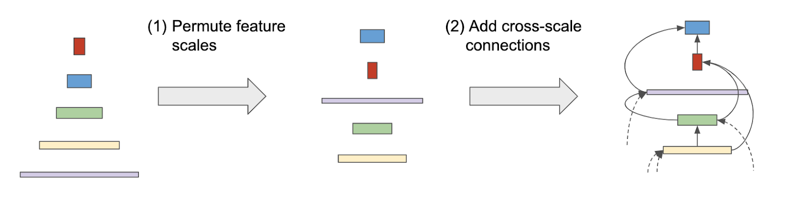
Utilizing the vision transformer (ViT-S/16) architecture, Path Foundation was selected as the best performing model from the optimization and evaluation process described above (and illustrated in the figure below). This model thus provides an important balance between performance and model size to enable valuable and scalable use in generating embeddings over the many individual image patches of large pathology WSIs.

SSL training with pathology-specific optimizations for Path Foundation.

The value of domain-specific image representations can also be seen in the figure below, which shows the linear probing performance improvement of Path Foundation (as measured by AUROC) compared to traditional pre-training on natural images (ImageNet-21k). This includes evaluation for tasks such as metastatic breast cancer detection in lymph nodes, prostate cancer grading, and breast cancer grading, among others.

Path Foundation embeddings significantly outperform traditional ImageNet embeddings as evaluated by linear probing across multiple evaluation tasks in histopathology.


Derm Foundation

Derm Foundation is an embedding tool derived from our research in applying DL to interpret images of dermatology conditions and includes our recent work that adds improvements to generalize better to new datasets. Due to its dermatology-specific pre-training it has a latent understanding of features present in images of skin conditions and can be used to quickly develop models to classify skin conditions. The model underlying the API is a BiT ResNet-101x3 trained in two stages. The first pre-training stage uses contrastive learning, similar to ConVIRT, to train on a large number of image-text pairs from the internet. In the second stage, the image component of this pre-trained model is then fine-tuned for condition classification using clinical datasets, such as those from teledermatology services.

Unlike histopathology images, dermatology images more closely resemble the real-world images used to train many of today's computer vision models. However, for specialized dermatology tasks, creating a high-quality model may still require a large dataset. With Derm Foundation, researchers can use their own smaller dataset to retrieve domain-specific embeddings, and use those to build smaller models (e.g., linear classifiers or other small non-linear models) that enable them to validate their research or product ideas. To evaluate this approach, we trained models on a downstream task using teledermatology data. Model training involved varying dataset sizes (12.5%, 25%, 50%, 100%) to compare embedding-based linear classifiers against fine-tuning.

The modeling variants considered were:

  • A linear classifier on frozen embeddings from BiT-M (a standard pre-trained image model)
  • Fine-tuned version of BiT-M with an extra dense layer for the downstream task
  • A linear classifier on frozen embeddings from the Derm Foundation API
  • Fine-tuned version of the model underlying the Derm Foundation API with an extra layer for the downstream task

We found that models built on top of the Derm Foundation embeddings for dermatology-related tasks achieved significantly higher quality than those built solely on embeddings or fine tuned from BiT-M. This advantage was found to be most pronounced for smaller training dataset sizes.

These results demonstrate that the Derm Foundation tooI can serve as a useful starting point to accelerate skin-related modeling tasks. We aim to enable other researchers to build on the underlying features and representations of dermatology that the model has learned.

However, there are limitations with this analysis. We're still exploring how well these embeddings generalize across task types, patient populations, and image settings. Downstream models built using Derm Foundation still require careful evaluation to understand their expected performance in the intended setting.


Access Path and Derm Foundation

We envision that the Derm Foundation and Path Foundation embedding tools will enable a range of use cases, including efficient development of models for diagnostic tasks, quality assurance and pre-analytical workflow improvements, image indexing and curation, and biomarker discovery and validation. We are releasing both tools to the research community so they can explore the utility of the embeddings for their own dermatology and pathology data.

To get access, please sign up to each tool's terms of service using the following Google Forms.

After gaining access to each tool, you can use the API to retrieve embeddings from dermatology images or digital pathology images stored in Google Cloud. Approved users who are just curious to see the model and embeddings in action can use the provided example Colab notebooks to train models using public data for classifying six common skin conditions or identifying tumors in histopathology patches. We look forward to seeing the range of use-cases these tools can unlock.


Acknowledgements

We would like to thank the many collaborators who helped make this work possible including Yun Liu, Can Kirmizi, Fereshteh Mahvar, Bram Sterling, Arman Tajback, Kenneth Philbrik, Arnav Agharwal, Aurora Cheung, Andrew Sellergren, Boris Babenko, Basil Mustafa, Jan Freyberg, Terry Spitz, Yuan Liu, Pinal Bavishi, Ayush Jain, Amit Talreja, Rajeev Rikhye, Abbi Ward, Jeremy Lai, Faruk Ahmed, Supriya Vijay,Tiam Jaroensri, Jessica Loo, Saurabh Vyawahare, Saloni Agarwal, Ellery Wulczyn, Jonathan Krause, Fayaz Jamil, Tom Small, Annisah Um'rani, Lauren Winer, Sami Lachgar, Yossi Matias, Greg Corrado, and Dale Webster.

Source: Google AI Blog


Introducing the Google Universal Image Embedding Challenge

Computer vision models see daily application for a wide variety of tasks, ranging from object recognition to image-based 3D object reconstruction. One challenging type of computer vision problem is instance-level recognition (ILR) — given an image of an object, the task is to not only determine the generic category of an object (e.g., an arch), but also the specific instance of the object (”Arc de Triomphe de l'Étoile, Paris, France”).

Previously, ILR was tackled using deep learning approaches. First, a large set of images was collected. Then a deep model was trained to embed each image into a high-dimensional space where similar images have similar representations. Finally, the representation was used to solve the ILR tasks related to classification (e.g., with a shallow classifier trained on top of the embedding) or retrieval (e.g., with a nearest neighbor search in the embedding space).

Since there are many different object domains in the world, e.g., landmarks, products, or artworks, capturing all of them in a single dataset and training a model that can distinguish between them is quite a challenging task. To decrease the complexity of the problem to a manageable level, the focus of research so far has been to solve ILR for a single domain at a time. To advance the research in this area, we hosted multiple Kaggle competitions focused on the recognition and retrieval of landmark images. In 2020, Amazon joined the effort and we moved beyond the landmark domain and expanded to the domains of artwork and product instance recognition. The next step is to generalize the ILR task to multiple domains.

To this end, we’re excited to announce the Google Universal Image Embedding Challenge, hosted by Kaggle in collaboration with Google Research and Google Lens. In this challenge, we ask participants to build a single universal image embedding model capable of representing objects from multiple domains at the instance level. We believe that this is the key for real-world visual search applications, such as augmenting cultural exhibits in a museum, organizing photo collections, visual commerce and more.

Images1 of object instances coming from multiple domains, which are represented in our dataset: apparel and accessories, packaged goods, furniture and home goods, toys, cars, landmarks, storefronts, dishes, artwork, memes and illustrations.

Degrees of Variation in Different Domains
To represent objects from a large number of domains, we require one model to learn many domain-specific subtasks (e.g., filtering different kinds of noise or focusing on a specific detail), which can only be learned from a semantically and visually diverse collection of images. Addressing each degree of variation proposes a new challenge for both image collection and model training.

The first sort of variation comes from the fact that while some domains contain unique objects in the world (landmarks, artwork, etc.), others contain objects that may have many copies (clothing, furniture, packaged goods, food, etc.). Because a landmark is always placed at the same location, the surrounding context may be useful for recognition. In contrast, a product, say a phone, even of a specific model and color, may have millions of physical instances and thus appear in many surrounding contexts.

Another challenge comes from the fact that a single object may appear different depending on the point of view, lighting conditions, occlusion or deformations (e.g., a dress worn on a person may look very different than on a hanger). In order for a model to learn invariance to all of these visual modes, all of them should be captured by the training data.

Additionally, similarities between objects differ across domains. For example, in order for a representation to be useful in the product domain, it must be able to distinguish very fine-grained details between similarly looking products belonging to two different brands. In the domain of food, however, the same dish (e.g., spaghetti bolognese) cooked by two chefs may look quite different, but the ability of the model to distinguish spaghetti bolognese from other dishes may be sufficient for the model to be useful. Additionally, a vision model of high quality should assign similar representations to more visually similar renditions of a dish.

Domain    Landmark    Apparel
Image      
Instance Name    Empire State Building2    Cycling jerseys with Android logo3

Which physical objects belong to the instance class?    Single instance in the world    Many physical instances; may differ in size or pattern (e.g., a patterned cloth cut differently)

What are the possible views of the object?    Appearance variation only based on capture conditions (e.g., illumination or viewpoint); limited number of common external views; possibility of many internal views    Deformable appearance (e.g., worn or not); limited number of common views: front, back, side

What are the surroundings and are they useful for recognition?    Surrounding context does not vary much other than daily and yearly cycles; may be useful for verifying the object of interest    Surrounding context can change dramatically due to difference in environment, additional pieces of clothing, or accessories partially occluding clothing of interest (e.g., a jacket or a scarf)

What may be tricky cases that do not belong to the instance class?    Replicas of landmarks (e.g., Eiffel Tower in Las Vegas), souvenirs    Same piece of apparel of different material or different color; visually very similar pieces with a small distinguishing detail (e.g., a small brand logo); different pieces of apparel worn by the same model
Variation among domains for landmark and apparel examples.

Learning Multi-domain Representations
After a collection of images covering a variety of domains is created, the next challenge is to train a single, universal model. Some features and tasks, such as representing color, are useful across many domains, and thus adding training data from any domain will likely help the model improve at distinguishing colors. Other features may be more specific to selected domains, thus adding more training data from other domains may deteriorate the model’s performance. For example, while for 2D artwork it may be very useful for the model to learn to find near duplicates, this may deteriorate the performance on clothing, where deformed and occluded instances need to be recognized.

The large variety of possible input objects and tasks that need to be learned require novel approaches for selecting, augmenting, cleaning and weighing the training data. New approaches for model training and tuning, and even novel architectures may be required.

Universal Image Embedding Challenge
To help motivate the research community to address these challenges, we are hosting the Google Universal Image Embedding Challenge. The challenge was launched on Kaggle in July and will be open until October, with cash prizes totaling $50k. The winning teams will be invited to present their methods at the Instance-Level Recognition workshop at ECCV 2022.

Participants will be evaluated on a retrieval task on a dataset of ~5,000 test query images and ~200,000 index images, from which similar images are retrieved. In contrast to ImageNet, which includes categorical labels, the images in this dataset are labeled at the instance level.

The evaluation data for the challenge is composed of images from the following domains: apparel and accessories, packaged goods, furniture and home goods, toys, cars, landmarks, storefronts, dishes, artwork, memes and illustrations.

Distribution of domains of query images.

We invite researchers and machine learning enthusiasts to participate in the Google Universal Image Embedding Challenge and join the Instance-Level Recognition workshop at ECCV 2022. We hope the challenge and the workshop will advance state-of-the-art techniques on multi-domain representations.

Acknowledgement
The core contributors to this project are Andre Araujo, Boris Bluntschli, Bingyi Cao, Kaifeng Chen, Mário Lipovský, Grzegorz Makosa, Mojtaba Seyedhosseini and Pelin Dogan Schönberger. We would like to thank Sohier Dane, Will Cukierski and Maggie Demkin for their help organizing the Kaggle challenge, as well as our ECCV workshop co-organizers Tobias Weyand, Bohyung Han, Shih-Fu Chang, Ondrej Chum, Torsten Sattler, Giorgos Tolias, Xu Zhang, Noa Garcia, Guangxing Han, Pradeep Natarajan and Sanqiang Zhao. Furthermore we are thankful to Igor Bonaci, Tom Duerig, Vittorio Ferrari, Victor Gomes, Futang Peng and Howard Zhou who gave us feedback, ideas and support at various points of this project.


1 Image credits: Chris Schrier, CC-BY; Petri Krohn, GNU Free Documentation License; Drazen Nesic, CC0; Marco Verch Professional Photographer, CCBY; Grendelkhan, CCBY; Bobby Mikul, CC0; Vincent Van Gogh, CC0; pxhere.com, CC0; Smart Home Perfected, CC-BY.  
2 Image credit: Bobby Mikul, CC0.  
3 Image credit: Chris Schrier, CC-BY.  

Source: Google AI Blog


Simplified Transfer Learning for Chest Radiography Model Development

Every year, nearly a billion chest X-ray (CXR) images are taken globally to aid in the detection and management of health conditions ranging from collapsed lungs to infectious diseases. Generally, CXRs are cheaper and more accessible than other forms of medical imaging. However, existing challenges continue to impede the optimal use of CXRs. For example, in some areas, trained radiologists that can accurately interpret CXR images are in short supply. In addition, interpretation variability between experts, workflow differences between institutions, and the presence of rare conditions familiar only to subspecialists all contribute to making high-quality CXR interpretation a challenge.

Recent research has leveraged machine learning (ML) to explore potential solutions for some of these challenges. There is significant interest and effort devoted to building deep learning models that detect abnormalities in CXRs and improve access, accuracy, and efficiency to identify diseases and conditions that affect the heart and lungs. However, building robust CXR models requires large labeled training datasets, which can be prohibitively expensive and time-consuming to create. In some cases, such as working with underrepresented populations or studying rare medical conditions, only limited data are available. Additionally, CXR images vary in quality across populations, geographies, and institutions, making it difficult to build robust models that perform well globally.

In “Simplified Transfer Learning for Chest Radiography Models Using Less Data”, published in the journal Radiology, we describe how Google Health utilizes advanced ML methods to generate pre-trained “CXR networks” that can convert CXR images to embeddings (i.e., information-rich numerical vectors) to enable the development of CXR models using less data and fewer computational resources. We demonstrate that even with less data and compute, this approach has enabled performance comparable to state-of-the-art deep learning models across various prediction tasks. We are also excited to announce the release of CXR Foundation, a tool that utilizes our CXR-specific network to enable developers to create custom embeddings for their CXR images. We believe this work will help accelerate the development of CXR models, aiding in disease detection and contributing to more equitable health access throughout the world.

Developing a Chest X-ray Network
A common approach to building medical ML models is to pre-train a model on a generic task using non-medical datasets and then refine the model on a target medical task. This process of transfer learning may improve the target task performance or at least speed up convergence by applying the understanding of natural images to medical images. However, transfer learning may still require large labeled medical datasets for the refinement step.

Expanding on this standard approach, our system supports modeling CXR-specific tasks through a three-step model training setup composed of (1) generic image pre-training similar to traditional transfer learning, (2) CXR-specific pre-training, and (3) task-specific training. The first and third steps are common in ML: first pre-training on a large dataset and labels that are not specific to the desired task, and then fine-tuning on the task of interest.

We built a CXR-specific image classifier that employs supervised contrastive learning (SupCon). SupCon pulls together representations of images that have the same label (e.g., abnormal) and pushes apart representations of images that have a different label (e.g., one normal image and one abnormal image). We pre-trained this model on de-identified CXR datasets of over 800,000 images generated in partnership with Northwestern Medicine and Apollo Hospitals in the US and India, respectively. We then leveraged noisy abnormality labels from natural language processing of radiology reports to build our “CXR-specific” network.

This network creates embeddings (i.e., information-rich numerical vectors that can be used to distinguish classes from each other) that can more easily train models for specific medical prediction tasks, such as image finding (e.g., airspace opacity), clinical condition (e.g., tuberculosis), or patient outcome (e.g., hospitalization). For example, the CXR network can generate embeddings for every image in a given CXR dataset. For these images, the generated embeddings and the labels for the desired target task (such as tuberculosis) are used as examples to train a small ML model.

Left: Training a CXR model for a given task generally requires a large number of labeled images and a significant amount of computational resources to create a foundation of neural network layers. Right: With the CXR network and tool providing this foundation, each new task requires only a fraction of the labeled images, computational resources, and neural network parameters compared to rebuilding the entire network from scratch.

Effects of CXR Pre-training
We visualized these embedding layers at each step of the process using airspace opacity as an example (see the figure below). Before SupCon-based pre-training, there was poor separation of normal and abnormal CXR embeddings. After SupCon-based pre-training, the positive examples were grouped more closely together, and the negative examples more closely together as well, indicating that the model had identified that images from each category resembled themselves.

Visualizations of the t-distributed stochastic neighbor embedding for generic vs. CXR-specific network embeddings. Embeddings are information-rich numerical vectors that alone can distinguish classes from each other, in this case, airspace opacity positive vs. negative.

Our research suggests that adding the second stage of pre-training enables high-quality models to be trained with up to 600-fold less data in comparison to traditional transfer learning approaches that leverage pre-trained models on generic, non-medical datasets. We found this to be true regardless of model architecture (e.g., ResNet or EfficientNet) or dataset used for natural image pre-training (e.g., ImageNet or JFT-300M). With this approach, researchers and developers can significantly reduce dataset size requirements.

Top: In a deep learning model, the neural network contains multiple layers of artificial neurons, with the first layer taking the CXR image as input, intermediate layers doing additional computation, and the final layer making the classification (e.g., airspace opacity: present vs. absent). The embedding layer is usually one of the last layers. Bottom left: The traditional transfer learning approach involves a two-step training setup where a generic pre-trained network is optimized directly on a prediction task of interest. Our proposed three-step training setup generates a CXR network using a SupCon ML technique (step 2) before optimization for prediction tasks of interest (step 3). Bottom right: Using the embeddings involves either training smaller models (the first two strategies) or fine-tuning the whole network if there are sufficient data (strategy 3).

Results
After training the initial model, we measured performance using the area under the curve (AUC) metric with both linear and non-linear models applied to CXR embeddings; and a non-linear model produced by fine-tuning the entire network. On public datasets, such as ChestX-ray14 and CheXpert, our work substantially and consistently improved the data-accuracy tradeoff for models developed across a range of training dataset sizes and several findings. For example, when evaluating the tool’s ability to develop tuberculosis models, data efficiency gains were more striking: models trained on the embeddings of just 45 images achieved non-inferiority to radiologists in detecting tuberculosis on an external validation dataset. For both tuberculosis and severe COVID-19 outcomes, we show that non-linear classifiers trained on frozen embeddings outperformed a model that was fine-tuned on the entire dataset.

Comparing CXR-specific networks for transfer learning (red), with a baseline transfer learning approach (blue) across a variety of CXR abnormalities (top left), tuberculosis (bottom left), and COVID-19 outcomes (bottom right). This approach improves performance at the same dataset size, or reduces the dataset size required to reach the same performance. Interestingly, using the CXR network with simpler ML models that are faster to train (red) performs better than training the full network (black) at dataset sizes up to 85 images.

Conclusion and Future Work
To accelerate CXR modeling efforts with low data and computational requirements, we are releasing our CXR Foundation tool, along with scripts to train linear and nonlinear classifiers. Via these embeddings, this tool will allow researchers to jump-start CXR modeling efforts using simpler transfer learning methods. This approach can be particularly useful for predictive modeling using small datasets, and for adapting CXR models when there are distribution shifts in patient populations (whether over time or across different institutions). We are excited to continue working with partners, such as Northwestern Medicine and Apollo Hospitals, to explore the impact of this technology further. By enabling researchers with limited data and compute to develop CXR models, we're hoping more developers can solve the most impactful problems for their populations.

Acknowledgements
Key contributors to this project at Google include Christina Chen, Yun Liu, Dilip Krishnan, Zaid Nabulsi, Atilla Kiraly, Arnav Agharwal, Eric Wu, Yuanzhen Li, Aaron Maschinot, Aaron Sarna, Jenny Huang, Marilyn Zhang, Charles Lau, Neeral Beladia, Daniel Tse, Krish Eswaran, and Shravya Shetty. Significant contributions and input were also made by collaborators Sreenivasa Raju Kalidindi, Mozziyar Etemadi, Florencia Garcia-Vicente, and David Melnick. For the ChestX-ray14 dataset, we thank the NIH Clinical Center for making it publicly available. The authors would also like to acknowledge many members of the Google Health Radiology and labeling software teams. Sincere appreciation also goes to the radiologists who enabled this work with their image interpretation and annotation efforts throughout the study; Jonny Wong for coordinating the imaging annotation work; Craig Mermel and Akinori Mitani for providing feedback on the manuscript; Nicole Linton and Lauren Winer for feedback on the blogpost; and Tom Small for the animation.

Source: Google AI Blog


LIMoE: Learning Multiple Modalities with One Sparse Mixture of Experts Model

Sparse models stand out among the most promising approaches for the future of deep learning. Instead of every part of a model processing every input (“dense” modeling), sparse models employing conditional computation learn to route individual inputs to different “experts” in a potentially huge network. This has many benefits. First, model size can increase while keeping computational cost constant — an effective and environmentally friendlier way to scale models, which is often key to high performance. Sparsity also naturally compartmentalizes neural networks. Dense models that learn many different tasks simultaneously (multitask) or sequentially (continual learning) often suffer negative interference, where too much task variety means it is better to just train one model per task, or catastrophic forgetting, where the model becomes worse at earlier tasks as new ones are added. Sparse models help avoid both these phenomena — by not applying the whole model to all inputs, “experts” in the model can specialize on different tasks or data types while still taking advantage of shared parts of the model.

Research on sparsity has long been pursued at Google Research. Pathways summarizes the research vision of building one single large model that diligently handles thousands of tasks and numerous data modalities. So far there has been considerable progress in sparse unimodal models for language (Switch, Task-MoE, GLaM) and computer vision (Vision MoE). Today, we take another important step towards the Pathways vision by studying large sparse models that simultaneously handle images and text with modality-agnostic routing. A relevant approach is multimodal contrastive learning, which requires a solid understanding of both images and text in order to align pictures with their correct text description. The strongest models that tackle this task to date rely on independent networks for each modality (a “two-tower” approach).

In “Multimodal Contrastive Learning with LIMoE: the Language Image Mixture of Experts”, we present the first large-scale multimodal architecture using a sparse mixture of experts. It simultaneously processes both images and text, but uses sparsely activated experts that naturally specialize. On zero-shot image classification, LIMoE outperforms both comparable dense multimodal models and two-tower approaches. The largest LIMoE achieves 84.1% zero-shot ImageNet accuracy, comparable to more expensive state-of-the-art models. Sparsity enables LIMoE to scale up gracefully and learn to handle very different inputs, addressing the tension between being a jack-of-all-trades generalist and a master-of-one specialist.

The LIMoE architecture contains many “experts” and routers decide which tokens (parts of an image or sentence) go to which experts. After being processed by expert layers (gray) and shared dense layers (brown), a final output layer computes a single vector representation for either an image or a text.

Sparse Mixture of Expert Models
Transformers represent data as a sequence of vectors (or tokens). Though originally developed for text, they can be applied to most things that are representable as a sequence of tokens, e.g., images, videos, and audio. Recent large-scale MoE models add expert layers to the Transformer architecture (e.g., gShard and ST-MoE in natural language processing, and Vision MoE for vision tasks).

A standard Transformer consists of many “blocks”, each containing various different layers. One of these layers is a feed-forward network (FFN). For LIMoE and the works cited above, this single FFN is replaced by an expert layer that contains many parallel FFNs, each of which is an expert. Given a sequence of tokens to process, a simple router learns to predict which experts should handle which tokens. Only a small number of experts are activated per token, meaning although the model capacity is significantly increased by virtue of having so many experts, the actual computational cost is controlled by using them sparsely. If only one expert is activated, the model's cost is roughly equivalent to the standard Transformer model.

LIMoE does precisely that, activating one expert per example, thereby matching the computational cost of the dense baselines. What’s different is that the LIMoE router might see tokens of either image or text data.

A unique failure mode of MoE models occurs when they try to send all tokens to the same expert. Typically this is addressed with auxiliary losses, extra training objectives that encourage balanced expert usage. We found that dealing with multiple modalities interacted with sparsity to cause new failure modes that existing auxiliary losses could not address. To overcome this, we developed new auxiliary losses (more details in the paper) and used routing prioritization (BPR) during training, two innovations that resulted in stable and high performance multimodal models.

The new auxiliary losses (LIMoE aux) and routing prioritization (BPR) stabilized and improved overall performance (left) and increased the success rate of routing behavior (middle and right). A low success rate means the router does not use all the experts available and drops many tokens due to individual expert capacity being reached, which usually indicates the sparse model is not learning well. The combination introduced for LIMoE ensures high routing success rates for both images and text and consequently leads to significantly better performance.

Contrastive Learning with LIMoE
In multimodal contrastive learning, models are trained on paired image-text data (e.g., a photo and its caption). Typically, an image model extracts a representation of images, and a different text model extracts a representation of text. The contrastive learning objective encourages the image and text representations to be close for the same image-text pair and far away for content from different pairs. Such models with aligned representations can be adapted to new tasks without extra training data (“zero-shot”), e.g., an image will be classified as a dog if its representation is closer to the representation of the word “dog” than the word “cat”. This idea scales to thousands of classes and is referred to as zero-shot image classification.

CLIP and ALIGN (both two-tower models) scaled this process to achieve 76.2% and 76.4% zero-shot classification accuracy on the popular ImageNet dataset. We study one-tower models which compute both image and text representations. We find this reduces performance for dense models, likely due to negative interference or insufficient capacity. However, a compute-matched LIMoE not only improves over the one-tower dense model, but also outperforms two-tower dense models. We trained a series of models in a comparable training regimen to CLIP. Our dense L/16 model achieves 73.5% zero-shot accuracy, whereas LIMoE-L/16 gets to 78.6%, even outperforming CLIP’s more expensive, two-tower L/14 model (76.2%). As shown below, LIMoE’s use of sparsity provides a remarkable performance boost over dense models with equivalent cost.

For a given compute cost (x-axis), LIMoE models (circles, solid line) are significantly better than their dense baselines (triangles, dashed line). The architecture indicates the size of the underlying transformer, increasing from left (S/32) to right (L/16). Following standard convention, S (small), B (base), and L (large) refer to model scale. The number refers to the patch size, where smaller patches imply a larger architecture.

LiT and BASIC pushed zero-shot accuracy for dense two-tower models to 84.5% and 85.6% respectively. In addition to scaling, these approaches made use of specialized pre-training methods, repurposing image models that were already of exceptionally high quality. LIMoE-H/14 does not benefit from any pre-training or modality-specific components, but still achieved a comparable 84.1% zero-shot accuracy training from scratch. The scale of these models is also interesting to compare: LiT and BASIC are 2.1B and 3B parameter models. LIMoE-H/14 has 5.6B parameters in total, but via sparsity it only applies 675M parameters per token making it significantly more lightweight.

Data seen during training
Model   Pre-training     Image-text     Total      Parameters per token     ImageNet accuracy  
CLIP - 12.8B 12.8B ~200M 76.2%
ALIGN - 19.8B 19.8B ~410M 76.4%
LiT 25.8B 18.2B 44.0B 1.1B 84.5%
BASIC 19.7B 32.8B 52.5B 1.5B 85.6%
LIMoE H/14    - 23.3B 23.3B 675M 84.1%

Understanding LIMoE’s Behavior
LIMoE was motivated by the intuition that sparse conditional computation enables a generalist multimodal model to still develop the specialization needed to excel at understanding each modality. We analyzed LIMoE’s expert layers and uncovered a few interesting phenomena.

First, we see the emergence of modality-specialized experts. In our training setup there are many more image tokens than text tokens, so all experts tend to process at least some images, but some experts process either mostly images, mostly text, or both.

Distributions for an eight expert LIMoE; percentages indicate the amount of image tokens processed by the expert. There are one or two experts clearly specialized on text (shown by the mostly blue experts), usually two to four image specialists (mostly red), and the remainder are somewhere in the middle.

There are also some clear qualitative patterns among the image experts — e.g., in most LIMoE models, there is an expert that processes all image patches that contain text. In the example below, one expert processes fauna and greenery, and another processes human hands.

LIMoE chooses an expert for each token. Here we show which image tokens go to which experts on one of the layers of LIMoE-H/14. Despite not being trained to do so, we observe the emergence of semantic experts that specialize in specific topics such as plants or wheels.

Moving Forward
Multimodal models that handle many tasks are a promising route forward, and there are two key ingredients for success: scale, and the ability to avoid interference between distinct tasks and modalities while taking advantage of synergies. Sparse conditional computation is an excellent way of doing both. It enables performant and efficient generalist models that also have the capacity and flexibility for the specialization necessary to excel at individual tasks, as demonstrated by LIMoE’s solid performance with less compute.

Acknowledgements
We thank our co-authors on this work: Joan Puigcerver, Rodolphe Jenatton and Neil Houlsby. We also thank Andreas Steiner, Xiao Wang and Xiaohua Zhai, who led early explorations into dense single-tower models for contrastive multimodal learning, and also were instrumental in providing data access. We enjoyed useful discussions with André Susano Pinto, Maxim Neumann, Barret Zoph, Liam Fedus, Wei Han and Josip Djolonga. Finally, we would also like to thank and acknowledge Tom Small for the awesome animated figure used in this post.

Source: Google AI Blog


Image-Text Pre-training with Contrastive Captioners

Oftentimes, machine learning (ML) model developers begin their design using a generic backbone model that is trained at scale and with capabilities transferable to a wide range of downstream tasks. In natural language processing, a number of popular backbone models, including BERT, T5, GPT-3 (sometimes also referred to as “foundation models”), are pre-trained on web-scale data and have demonstrated generic multi-tasking capabilities through zero-shot, few-shot or transfer learning. Compared with training over-specialized individual models, pre-training backbone models for a large number of downstream tasks can amortize the training costs, allowing one to overcome resource limitations when building large scale models.

In computer vision, pioneering work has shown the effectiveness of single-encoder models pre-trained for image classification to capture generic visual representations that are effective for other downstream tasks. More recently, contrastive dual-encoder (CLIP, ALIGN, Florence) and generative encoder-decoder (SimVLM) approaches trained using web-scale noisy image-text pairs have been explored. Dual-encoder models exhibit remarkable zero-shot image classification capabilities but are less effective for joint vision-language understanding. On the other hand, encoder-decoder methods are good at image captioning and visual question answering but cannot perform retrieval-style tasks.

In “CoCa: Contrastive Captioners are Image-Text Foundation Models”, we present a unified vision backbone model called Contrastive Captioner (CoCa). Our model is a novel encoder-decoder approach that simultaneously produces aligned unimodal image and text embeddings and joint multimodal representations, making it flexible enough to be directly applicable for all types of downstream tasks. Specifically, CoCa achieves state-of-the-art results on a series of vision and vision-language tasks spanning vision recognition, cross-modal alignment, and multimodal understanding. Furthermore, it learns highly generic representations so that it can perform as well or better than fully fine-tuned models with zero-shot learning or frozen encoders.

Overview of Contrastive Captioners (CoCa) compared to single-encoder, dual-encoder and encoder-decoder models.

Method
We propose CoCa, a unified training framework that combines contrastive loss and captioning loss on a single training data stream consisting of image annotations and noisy image-text pairs, effectively merging single-encoder, dual-encoder and encoder-decoder paradigms.

To this end, we present a novel encoder-decoder architecture where the encoder is a vision transformer (ViT), and the text decoder transformer is decoupled into two parts, a unimodal text decoder and a multimodal text decoder. We skip cross-attention in unimodal decoder layers to encode text-only representations for contrastive loss, and cascade multimodal decoder layers with cross-attention to image encoder outputs to learn multimodal image-text representations for captioning loss. This design maximizes the model's flexibility and universality in accommodating a wide spectrum of tasks, and at the same time, it can be efficiently trained with a single forward and backward propagation for both training objectives, resulting in minimal computational overhead. Thus, the model can be trained end-to-end from scratch with training costs comparable to a naïve encoder-decoder model.

Illustration of forward propagation used by CoCa for both contrastive and captioning losses.

Benchmark Results
The CoCa model can be directly fine-tuned on many tasks with minimal adaptation. By doing so, our model achieves a series of state-of-the-art results on popular vision and multimodal benchmarks, including (1) visual recognition: ImageNet, Kinetics-400/600/700, and MiT; (2) cross-modal alignment: MS-COCO, Flickr30K, and MSR-VTT; and (3) multimodal understanding: VQA, SNLI-VE, NLVR2, and NoCaps.

Comparison of CoCa with other image-text backbone models (without task-specific customization) and multiple state-of-the-art task-specialized models.

It is noteworthy that CoCa attains these results as a single model adapted for all tasks while often lighter than prior top-performing specialized models. For example, CoCa obtains 91.0% ImageNet top-1 accuracy while using less than half the parameters of prior state-of-the-art models. In addition, CoCa also obtains strong generative capability of high-quality image captions.

Image classification scaling performance comparing fine-tuned ImageNet top-1 accuracy versus model size.
Text captions generated by CoCa with NoCaps images as input.

Zero-Shot Performance
Besides achieving excellent performance with fine-tuning, CoCa also outperforms previous state-of-the-art models on zero-shot learning tasks, including image classification,and cross-modal retrieval. CoCa obtains 86.3% zero-shot accuracy on ImageNet while also robustly outperforming prior models on challenging variant benchmarks, such as ImageNet-A, ImageNet-R, ImageNet-V2, and ImageNet-Sketch. As shown in the figure below, CoCa obtains better zero-shot accuracy with smaller model sizes compared to prior methods.

Image classification scaling performance comparing zero-shot ImageNet top-1 accuracy versus model size.

Frozen Encoder Representation
One particularly exciting observation is that CoCa achieves results comparable to the best fine-tuned models using only a frozen visual encoder, in which features extracted after model training are used to train a classifier, rather than the more computationally intensive effort of fine-tuning a model. On ImageNet, a frozen CoCa encoder with a learned classification head obtains 90.6% top-1 accuracy, which is better than the fully fine-tuned performance of existing backbone models (90.1%). We also find this setup to work extremely well for video recognition. We feed sampled video frames into the CoCa frozen image encoder individually, and fuse output features by attentional pooling before applying a learned classifier. This simple approach using a CoCa frozen image encoder achieves video action recognition top-1 accuracy of 88.0% on Kinetics-400 dataset and demonstrates that CoCa learns a highly generic visual representation with the combined training objectives.

Comparison of Frozen CoCa visual encoder with (multiple) best-performing fine-tuned models.

Conclusion
We present Contrastive Captioner (CoCa), a novel pre-training paradigm for image-text backbone models. This simple method is widely applicable to many types of vision and vision-language downstream tasks, and obtains state-of-the-art performance with minimal or even no task-specific adaptations.

Acknowledgements
We would like to thank our co-authors Vijay Vasudevan, Legg Yeung, Mojtaba Seyedhosseini, and Yonghui Wu who have been involved in all aspects of the project. We also would like to thank Yi-Ting Chen, Kaifeng Chen, Ye Xia, Zhen Li, Chao Jia, Yinfei Yang, Zhengdong Zhang, Wei Han, Yuan Cao, Tao Zhu, Futang Peng, Soham Ghosh, Zihang Dai, Xin Li, Anelia Angelova, Jason Baldridge, Izhak Shafran, Shengyang Dai, Abhijit Ogale, Zhifeng Chen, Claire Cui, Paul Natsev, Tom Duerig for helpful discussions, Andrew Dai for help with contrastive models, Christopher Fifty and Bowen Zhang for help with video models, Yuanzhong Xu for help with model scaling, Lucas Beyer for help with data preparation, Andy Zeng for help with MSR-VTT evaluation, Hieu Pham and Simon Kornblith for help with zero-shot evaluations, Erica Moreira and Victor Gomes for help with resource coordination, Liangliang Cao for proofreading, Tom Small for creating the animations used in this blogpost, and others in the Google Brain team for support throughout this project.

Source: Google AI Blog


Extending Contrastive Learning to the Supervised Setting

In recent years, self-supervised representation learning, which is used in a variety of image and video tasks, has significantly advanced due to the application of contrastive learning. These contrastive learning approaches typically teach a model to pull together the representations of a target image (a.k.a., the “anchor”) and a matching (“positive”) image in embedding space, while also pushing apart the anchor from many non-matching (“negative”) images. Because labels are assumed to be unavailable in self-supervised learning, the positive is often an augmentation of the anchor, and the negatives are chosen to be the other samples from the training minibatch. However, because of this random sampling, false negatives, i.e., negatives generated from samples of the same class as the anchor, can cause a degradation in the representation quality. Furthermore, determining the optimal method to generate positives is still an area of active research.

In contrast to the self-supervised approach, a fully-supervised approach could use labeled data to generate positives from existing same-class examples, providing more variability in pretraining than could typically be achieved by simply augmenting the anchor. However, very little work has been done to successfully apply contrastive learning in the fully-supervised domain.

In “Supervised Contrastive Learning”, presented at NeurIPS 2020, we propose a novel loss function, called SupCon, that bridges the gap between self-supervised learning and fully supervised learning and enables contrastive learning to be applied in the supervised setting. Leveraging labeled data, SupCon encourages normalized embeddings from the same class to be pulled closer together, while embeddings from different classes are pushed apart. This simplifies the process of positive selection, while avoiding potential false negatives. Because it accommodates multiple positives per anchor, this approach results in an improved selection of positive examples that are more varied, while still containing semantically relevant information. SupCon also allows label information to play an active role in representation learning rather than restricting it to be used only in downstream training, as is the case for conventional contrastive learning. To the best of our knowledge, this is the first contrastive loss to consistently perform better on large-scale image classification problems than the common approach of using cross-entropy loss to train the model directly. Importantly, SupCon is straightforward to implement and stable to train, provides consistent improvement to top-1 accuracy for a number of datasets and architectures (including Transformer architectures), and is robust to image corruptions and hyperparameter variations.

Self-supervised (left) vs supervised (right) contrastive losses: The self-supervised contrastive loss contrasts a single positive for each anchor (i.e., an augmented version of the same image) against a set of negatives consisting of the entire remainder of the minibatch. The supervised contrastive loss considered in this paper, however, contrasts the set of all samples from the same class as positives against the negatives from the remainder of the batch.

The Supervised Contrastive Learning Framework
SupCon can be seen as a generalization of both the SimCLR and N-pair losses — the former uses positives generated from the same sample as that of the anchor, and the latter uses positives generated from different samples by exploiting known class labels. The use of many positives and many negatives for each anchor allows SupCon to achieve state-of-the-art performance without the need for hard negative mining (i.e., searching for negatives similar to the anchor), which can be difficult to tune properly.

SupCon subsumes multiple losses from the literature and is a generalization of the SimCLR and N-Pair losses.

This method is structurally similar to those used in self-supervised contrastive learning, with modifications for supervised classification. Given an input batch of data, we first apply data augmentation twice to obtain two copies, or “views,” of each sample in the batch (though one could create and use any number of augmented views). Both copies are forward propagated through an encoder network, and the resulting embedding is then L2-normalized. Following standard practice, the representation is further propagated through an optional projection network to help identify meaningful features. The supervised contrastive loss is computed on the normalized outputs of the projection network. Positives for an anchor consist of the representations originating from the same batch instance as the anchor or from other instances with the same label as the anchor; the negatives are then all remaining instances. To measure performance on downstream tasks, we train a linear classifier on top of the frozen representations.

Cross-entropy, self-supervised contrastive loss and supervised contrastive loss Left: The cross-entropy loss uses labels and a softmax loss to train a classifier. Middle: The self-supervised contrastive loss uses a contrastive loss and data augmentations to learn representations. Right: The supervised contrastive loss also learns representations using a contrastive loss, but uses label information to sample positives in addition to augmentations of the same image.

Key Findings
SupCon consistently boosts top-1 accuracy compared to cross-entropy, margin classifiers (with use of labels), and self-supervised contrastive learning techniques on CIFAR-10 and CIFAR-100 and ImageNet datasets. With SupCon, we achieve excellent top-1 accuracy on the ImageNet dataset with the ResNet-50 and ResNet-200 architectures. On ResNet-200, we achieve a top-1 accuracy of 81.4%, which is a 0.8% improvement over the state-of-the-art cross-entropy loss using the same architecture (which represents a significant advance for ImageNet). We also compared cross-entropy and SupCon on a Transformer-based ViT-B/16 model and found a consistent improvement over cross-entropy (77.8% versus 76% for ImageNet; 92.6% versus 91.6% for CIFAR-10) under the same data augmentation regime (without any higher-resolution fine-tuning).

The SupCon loss consistently outperforms cross-entropy with standard data augmentation strategies (AutoAugment, RandAugment and CutMix). We show top-1 accuracy for ImageNet, on ResNet-50, ResNet-101 and ResNet200.

We also demonstrate analytically that the gradient of our loss function encourages learning from hard positives and hard negatives. The gradient contributions from hard positives/negatives are large while those for easy positives/negatives are small. This implicit property allows the contrastive loss to sidestep the need for explicit hard mining, which is a delicate but critical part of many losses, such as triplet loss. See the supplementary material of our paper for a full derivation.

SupCon is also more robust to natural corruptions, such as noise, blur and JPEG compression. The mean Corruption Error (mCE) measures the average degradation in performance compared to the benchmark ImageNet-C dataset. The SupCon models have lower mCE values across different corruptions compared to cross-entropy models, showing increased robustness.

We show empirically that the SupCon loss is less sensitive than cross-entropy to a range of hyperparameters. Across changes in augmentations, optimizers, and learning rates, we observe significantly lower variance in the output of the contrastive loss. Moreover, applying different batch sizes while holding all other hyperparameters constant results in consistently better top-1 accuracy of SupCon to that of cross-entropy at each batch size.

Accuracy of cross-entropy and supervised contrastive loss as a function of hyperparameters and training data size, measured on ImageNet with a ResNet-50 encoder. Left: Boxplot showing Top-1 accuracy vs changes in augmentation, optimizer and learning rates. SupCon yields more consistent results across variations in each, which is useful when the best strategies are unknown a priori. Right: Top-1 accuracy as a function of batch size shows both losses benefit from larger batch sizes while SupCon has higher Top-1 accuracy, even when trained with small batch sizes.
Accuracy of supervised contrastive loss as a function of training duration and the temperature hyperparameter, measured on ImageNet with a ResNet-50 encoder. Left: Top-1 accuracy as a function of SupCon pre-training epochs. Right: Top-1 accuracy as a function of temperature during the pre-training stage for SupCon. Temperature is an important hyperparameter in contrastive learning and reducing sensitivity to temperature is desirable.

Broader Impact and Next Steps
This work provides a technical advancement in the field of supervised classification. Supervised contrastive learning can improve both the accuracy and robustness of classifiers with minimal complexity. The classic cross-entropy loss can be seen as a special case of SupCon where the views correspond to the images and the learned embeddings in the final linear layer corresponding to the labels. We note that SupCon benefits from large batch sizes, and being able to train the models on smaller batches is an important topic for future research.

Our Github repository includes Tensorflow code to train the models in the paper. Our pre-trained models are also released on TF-Hub.

Acknowledgements
The NeurIPS paper was jointly co-authored with Prannay Khosla, Piotr Teterwak, Chen Wang, Aaron Sarna, Yonglong Tian, Phillip Isola, Aaron Maschinot, Ce Liu, and Dilip Krishnan. Special thanks to Jenny Huang for leading the writing process for this blogpost.

Source: Google AI Blog


Uncovering Unknown Unknowns in Machine Learning

The performance of machine learning (ML) models depends both on the learning algorithms, as well as the data used for training and evaluation. The role of the algorithms is well studied and the focus of a multitude of challenges, such as SQuAD, GLUE, ImageNet, and many others. In addition, there have been efforts to also improve the data, including a series of workshops addressing issues for ML evaluation. In contrast, research and challenges that focus on the data used for evaluation of ML models are not commonplace. Furthermore, many evaluation datasets contain items that are easy to evaluate, e.g., photos with a subject that is easy to identify, and thus they miss the natural ambiguity of real world context. The absence of ambiguous real-world examples in evaluation undermines the ability to reliably test machine learning performance, which makes ML models prone to develop “weak spots”, i.e., classes of examples that are difficult or impossible for a model to accurately evaluate, because that class of examples is missing from the evaluation set.

To address the problem of identifying these weaknesses in ML models, we recently launched the Crowdsourcing Adverse Test Sets for Machine Learning (CATS4ML) Data Challenge at HCOMP 2020 (open until 30 April, 2021 to researchers and developers worldwide). The goal of the challenge is to raise the bar in ML evaluation sets and to find as many examples as possible that are confusing or otherwise problematic for algorithms to process. CATS4ML relies on people’s abilities and intuition to spot new data examples about which machine learning is confident, but actually misclassifies.

What are ML “Weak Spots”?
There are two categories of weak spots: known unknowns and unknown unknowns. Known unknowns are examples for which a model is unsure about the correct classification. The research community continues to study this in a field known as active learning, and has found the solution to be, in very general terms, to interactively solicit new labels from people on uncertain examples. For example, if a model is not certain whether or not the subject of a photo is a cat, a person is asked to verify; but if the system is certain, a person is not asked. While there is room for improvement in this area, what is comforting is that the confidence of the model is correlated with its performance, i.e., one can see what the model doesn’t know.

Unknown unknowns, on the other hand, are examples where a model is confident about its answer, but is actually wrong. Efforts to proactively discover unknown unknowns (e.g., Attenberg 2015 and Crawford 2019) have helped uncover a multitude of unintended machine behaviours. In contrast to such approaches for the discovery of unknown unknowns, generative adversarial networks (GANs) generate unknown unknowns for image recognition models in the form of optical illusions for computers that cause deep learning models to make mistakes beyond human perception. While GANs uncover model exploits in the event of an intentional manipulation, real-world examples can better highlight a model’s failures in its day-to-day performance. These real-world examples are the unknown unknowns of interest to CATS4ML — the challenge aims to gather unmanipulated examples that humans can reliably interpret but on which many ML models would confidently disagree.

Example illustrating how optical illusions for computers caused by adversarial noise help discover machine manipulated unknown unknowns for ML models (based on Brown 2018).

First Edition of CATS4ML Data Challenge: Open Images Dataset
The CATS4ML Data Challenge focuses on visual recognition, using images and labels from the Open Images Dataset. The target images for the challenge are selected from the Open Images Dataset along with a set of 24 target labels from the same dataset. The challenge participants are invited to invent new and creative ways to explore this existing publicly available dataset and, focussed on a list of pre-selected target labels, discover examples of unknown unknowns for ML models.

Examples from the Open Images Dataset as possible unknown unknowns for ML models.

CATS4ML is a complementary effort to FAIR’s recently introduced DynaBench research platform for dynamic data collection. Where DynaBench tackles issues with static benchmarks using ML models with humans in the loop, CATS4ML focuses on improving evaluation datasets for ML by encouraging the exploration of existing ML benchmarks for adverse examples that can be unknown unknowns. The results will help detect and avoid future errors, and also will give insights to model explainability.

In this way, CATS4ML aims to raise greater awareness of the problem by providing dataset resources that developers can use to uncover the weak spots of their algorithms. This will also inform researchers on how to create benchmark datasets for machine learning that are more balanced, diverse and socially aware.

Get Involved
We invite the global community of ML researchers and practitioners to join us in the effort of discovering interesting, difficult examples from the Open Images Dataset. Register on the challenge website, download the target images and labeled data, contribute the images you discover and join the competition for the winning participant!

To score points in this competition, participants should submit a set of image-label pairs that will be confirmed by human-in-the-loop raters, whose votes should be in disagreement with the average machine score for the label over a number of machine learning models.

An example of how a submitted image can score points. The same image can score as a false positive (Left) and as a false negative (Right) with two different labels. In both cases the human verification is in disagreement with the machine score. Participants score on submitted image-label pairs, which means that one and the same image can be an example of an ML unknown unknown for different labels.

The challenge is open until 30 April, 2021 to researchers and developers worldwide. To learn more about CATS4ML and how to join, please review these slides and visit the challenge website.

Acknowledgements
The release of the CATS4ML Data Challenge has been possible thanks to the hard work of a lot of people including, but not limited to, the following (in alphabetical order of last name): Osman Aka, Ken Burke, Tulsee Doshi, Mig Gerard, Victor Gomes, Shahab Kamali, Igor Karpov, Devi Krishna, Daphne Luong, Carey Radebaugh, Jamie Taylor, Nithum Thain, Kenny Wibowo, Ka Wong, and Tong Zhou.

Source: Google AI Blog


Advancing Instance-Level Recognition Research

Instance-level recognition (ILR) is the computer vision task of recognizing a specific instance of an object, rather than simply the category to which it belongs. For example, instead of labeling an image as “post-impressionist painting”, we’re interested in instance-level labels like “Starry Night Over the Rhone by Vincent van Gogh”, or “Arc de Triomphe de l'Étoile, Paris, France”, instead of simply “arch”. Instance-level recognition problems exist in many domains, like landmarks, artwork, products, or logos, and have applications in visual search apps, personal photo organization, shopping and more. Over the past several years, Google has been contributing to research on ILR with the Google Landmarks Dataset and Google Landmarks Dataset v2 (GLDv2), and novel models such as DELF and Detect-to-Retrieve.

Three types of image recognition problems, with different levels of label granularity (basic, fine-grained, instance-level), for objects from the artwork, landmark and product domains. In our work, we focus on instance-level recognition.

Today, we highlight some results from the Instance-Level Recognition Workshop at ECCV’20. The workshop brought together experts and enthusiasts in this area, with many fruitful discussions, some of which included our ECCV’20 paper “DEep Local and Global features” (DELG), a state-of-the-art image feature model for instance-level recognition, and a supporting open-source codebase for DELG and other related ILR techniques. Also presented were two new landmark challenges (on recognition and retrieval tasks) based on GLDv2, and future ILR challenges that extend to other domains: artwork recognition and product retrieval. The long-term goal of the workshop and challenges is to foster advancements in the field of ILR and push forward the state of the art by unifying research workstreams from different domains, which so far have mostly been tackled as separate problems.

DELG: DEep Local and Global Features
Effective image representations are the key components required to solve instance-level recognition problems. Often, two types of representations are necessary: global and local image features. A global feature summarizes the entire contents of an image, leading to a compact representation but discarding information about spatial arrangement of visual elements that may be characteristic of unique examples. Local features, on the other hand, comprise descriptors and geometry information about specific image regions; they are especially useful to match images depicting the same objects.

Currently, most systems that rely on both of these types of features need to separately adopt each of them using different models, which leads to redundant computations and lowers overall efficiency. To address this, we proposed DELG, a unified model for local and global image features.

The DELG model leverages a fully-convolutional neural network with two different heads: one for global features and the other for local features. Global features are obtained using pooled feature maps of deep network layers, which in effect summarize the salient features of the input images making the model more robust to subtle changes in input. The local feature branch leverages intermediate feature maps to detect salient image regions, with the help of an attention module, and to produce descriptors that represent associated localized contents in a discriminative manner.

Our proposed DELG model (left). Global features can be used in the first stage of a retrieval-based system, to efficiently select the most similar images (bottom). Local features can then be employed to re-rank top results (top, right), increasing the precision of the system.

This novel design allows for efficient inference since it enables extraction of global and local features within a single model. For the first time, we demonstrated that such a unified model can be trained end-to-end and deliver state-of-the-art results for instance-level recognition tasks. When compared to previous global features, this method outperforms other approaches by up to 7.5% mean average precision; and for the local feature re-ranking stage, DELG-based results are up to 7% better than previous work. Overall, DELG achieves 61.2% average precision on the recognition task of GLDv2, which outperforms all except two methods of the 2019 challenge. Note that all top methods from that challenge used complex model ensembles, while our results use only a single model.

Tensorflow 2 Open-Source Codebase
To foster research reproducibility, we are also releasing a revamped open-source codebase that includes DELG and other techniques relevant to instance-level recognition, such as DELF and Detect-to-Retrieve. Our code adopts the latest Tensorflow 2 releases, and makes available reference implementations for model training & inference, besides image retrieval and matching functionalities. We invite the community to use and contribute to this codebase in order to develop strong foundations for research in the ILR field.

New Challenges for Instance Level Recognition
Focused on the landmarks domain, the Google Landmarks Dataset v2 (GLDv2) is the largest available dataset for instance-level recognition, with 5 million images spanning 200 thousand categories. By training landmark retrieval models on this dataset, we have demonstrated improvements of up to 6% mean average precision, compared to models trained on earlier datasets. We have also recently launched a new browser interface for visually exploring the GLDv2 dataset.

This year, we also launched two new challenges within the landmark domain, one focusing on recognition and the other on retrieval. These competitions feature newly-collected test sets, and a new evaluation methodology: instead of uploading a CSV file with pre-computed predictions, participants have to submit models and code that are run on Kaggle servers, to compute predictions that are then scored and ranked. The compute restrictions of this environment put an emphasis on efficient and practical solutions.

The challenges attracted over 1,200 teams, a 3x increase over last year, and participants achieved significant improvements over our strong DELG baselines. On the recognition task, the highest scoring submission achieved a relative increase of 43% average precision score and on the retrieval task, the winning team achieved a 59% relative improvement of the mean average precision score. This latter result was achieved via a combination of more effective neural networks, pooling methods and training protocols (see more details on the Kaggle competition site).

In addition to the landmark recognition and retrieval challenges, our academic and industrial collaborators discussed their progress on developing benchmarks and competitions in other domains. A large-scale research benchmark for artwork recognition is under construction, leveraging The Met’s Open Access image collection, and with a new test set consisting of guest photos exhibiting various photometric and geometric variations. Similarly, a new large-scale product retrieval competition will capture various challenging aspects, including a very large number of products, a long-tailed class distribution and variations in object appearance and context. More information on the ILR workshop, including slides and video recordings, is available on its website.

With this research, open source code, data and challenges, we hope to spur progress in instance-level recognition and enable researchers and machine learning enthusiasts from different communities to develop approaches that generalize across different domains.

Acknowledgements
The main Google contributors of this project are André Araujo, Cam Askew, Bingyi Cao, Jack Sim and Tobias Weyand. We’d like to thank the co-organizers of the ILR workshop Ondrej Chum, Torsten Sattler, Giorgos Tolias (Czech Technical University), Bohyung Han (Seoul National University), Guangxing Han (Columbia University), Xu Zhang (Amazon), collaborators on the artworks dataset Nanne van Noord, Sarah Ibrahimi (University of Amsterdam), Noa Garcia (Osaka University), as well as our collaborators from the Metropolitan Museum of Art: Jennie Choi, Maria Kessler and Spencer Kiser. For the open-source Tensorflow codebase, we’d like to thank the help of recent contributors: Dan Anghel, Barbara Fusinska, Arun Mukundan, Yuewei Na and Jaeyoun Kim. We are grateful to Will Cukierski, Phil Culliton, Maggie Demkin for their support with the landmarks Kaggle competitions. Also we’d like to thank Ralph Keller and Boris Bluntschli for their help with data collection.

Source: Google AI Blog


SpineNet: A Novel Architecture for Object Detection Discovered with Neural Architecture Search


Convolutional neural networks created for image tasks typically encode an input image into a sequence of intermediate features that capture the semantics of an image (from local to global), where each subsequent layer has a lower spatial dimension. However, this scale-decreased model may not be able to deliver strong features for multi-scale visual recognition tasks where recognition and localization are both important (e.g., object detection and segmentation). Several works including FPN and DeepLabv3+ propose multi-scale encoder-decoder architectures to address this issue, where a scale-decreased network (e.g., a ResNet) is taken as the encoder (commonly referred to as a backbone model). A decoder network is then applied to the backbone to recover the spatial information.

While this architecture has yielded improved success for image recognition and localization tasks, it still relies on a scale-decreased backbone that throws away spatial information by down-sampling, which the decoder then must attempt to recover. What if one were to design an alternate backbone model that avoids this loss of spatial information, and is thus inherently well-suited for simultaneous image recognition and localization?

In our recent CVPR 2020 paper “SpineNet: Learning Scale-Permuted Backbone for Recognition and Localization”, we propose a meta architecture called a scale-permuted model that enables two major improvements on backbone architecture design. First, the spatial resolution of intermediate feature maps should be able to increase or decrease anytime so that the model can retain spatial information as it grows deeper. Second, the connections between feature maps should be able to go across feature scales to facilitate multi-scale feature fusion. We then use neural architecture search (NAS) with a novel search space design that includes these features to discover an effective scale-permuted model. We demonstrate that this model is successful in multi-scale visual recognition tasks, outperforming networks with standard, scale-reduced backbones. To facilitate continued work in this space, we have open sourced the SpineNet code to the Tensorflow TPU GitHub repository in Tensorflow 1 and TensorFlow Model Garden GitHub repository in Tensorflow 2.
A scale-decreased backbone is shown on the left and a scale-permuted backbone is shown on the right. Each rectangle represents a building block. Colors and shapes represent different spatial resolutions and feature dimensions. Arrows represent connections among building blocks.
Design of SpineNet Architecture
In order to efficiently design the architecture for SpineNet, and avoid a time-intensive manual search of what is optimal, we leverage NAS to determine an optimal architecture. The backbone model is learned on the object detection task using the COCO dataset, which requires simultaneous recognition and localization. During architecture search, we learn three things:
  • Scale permutations: The orderings of network building blocks are important because each block can only be built from those that already exist (i.e., with a “lower ordering”). We define the search space of scale permutations by rearranging intermediate and output blocks, respectively.
  • Cross-scale connections: We define two input connections for each block in the search space. The parent blocks can be any block with a lower ordering or a block from the stem network.
  • Block adjustments (optional): We allow the block to adjust its scale level and type.
The architecture search process from a scale-decreased backbone to a scale-permuted backbone.
Taking the ResNet-50 backbone as the seed for the NAS search, we first learn scale-permutation and cross-scale connections. All candidate models in the search space have roughly the same computation as ResNet-50 since we just permute the ordering of feature blocks to obtain candidate models. The learned scale-permuted model outperforms ResNet-50-FPN by +2.9% average precision (AP) in the object detection task. The efficiency can be further improved (-10% FLOPs) by adding search options to adjust scale and type (e.g., residual block or bottleneck block, used in the ResNet model family) of each candidate feature block.

We name the learned 49-layer scale-permuted backbone architecture SpineNet-49. SpineNet-49 can be further scaled up to SpineNet-96/143/190 by repeating blocks two, three, or four times and increasing the feature dimension. An architecture comparison between ResNet-50-FPN and the final SpineNet-49 is shown below.
The architecture comparison between a ResNet backbone (left) and the SpineNet backbone (right) derived from it using NAS.
Performance
We demonstrate the performance of SpineNet models through comparison with ResNet-FPN. Using similar building blocks, SpineNet models outperform their ResNet-FPN counterparts by ~3% AP at various scales while using 10-20% fewer FLOPs. In particular, our largest model, SpineNet-190, achieves 52.1% AP on COCO for a single model without multi-scale testing during inference, significantly outperforming prior detectors. SpineNet also transfers to classification tasks, achieving 5% top-1 accuracy improvement on the challenging iNaturalist fine-grained dataset.
Performance comparisons of SpineNet models and ResNet-FPN models adopting the RetinaNet detection framework on COCO bounding box detection.
Performance comparisons of SpineNet models and ResNet models on ImageNet classification and iNaturalist fine-grained image classification.
Conclusion
In this work, we identify that the conventional scale-decreased model, even with a decoder network, is not effective for simultaneous recognition and localization. We propose the scale-permuted model, a new meta-architecture, to address the issue. To prove the effectiveness of scale-permuted models, we learn SpineNet by Neural Architecture Search in object detection and demonstrate it can be used directly in image classification. In the future, we hope the scale-permuted model will become the meta-architecture design of backbones across many visual tasks beyond detection and classification.

Acknowledgements
Special thanks to the co-authors of the paper: Tsung-Yi Lin, Pengchong Jin, Golnaz Ghiasi, Mingxing Tan, Yin Cui, Quoc V. Le, and Xiaodan Song. We also would like to acknowledge Yeqing Li, Youlong Cheng, Jing Li, Jianwei Xie, Russell Power, Hongkun Yu, Chad Richards, Liang-Chieh Chen, Anelia Angelova, and the larger Google Brain Team for their help.

Source: Google AI Blog


Open-Sourcing BiT: Exploring Large-Scale Pre-training for Computer Vision


A common refrain for computer vision researchers is that modern deep neural networks are always hungry for more labeled data — current state-of-the-art CNNs need to be trained on datasets such as OpenImages or Places, which consist of over 1M labelled images. However, for many applications, collecting this amount of labeled data can be prohibitive to the average practitioner.

A common approach to mitigate the lack of labeled data for computer vision tasks is to use models that have been pre-trained on generic data (e.g., ImageNet). The idea is that visual features learned on the generic data can be re-used for the task of interest. Even though this pre-training works reasonably well in practice, it still falls short of the ability to both quickly grasp new concepts and understand them in different contexts. In a similar spirit to how BERT and T5 have shown advances in the language domain, we believe that large-scale pre-training can advance the performance of computer vision models.

In “Big Transfer (BiT): General Visual Representation Learning” we devise an approach for effective pre-training of general features using image datasets at a scale beyond the de-facto standard (ILSVRC-2012). In particular, we highlight the importance of appropriately choosing normalization layers and scaling the architecture capacity as the amount of pre-training data increases. Our approach exhibits unprecedented performance adapting to a wide range of new visual tasks, including the few-shot recognition setting and the recently introduced “real-world” ObjectNet benchmark. We are excited to share the best BiT models pre-trained on public datasets, along with code in TF2, Jax, and PyTorch. This will allow anyone to reach state-of-the-art performance on their task of interest, even with just a handful of labeled images per class.

Pre-training
In order to investigate the effect of data scale, we revisit common design choices of the pre-training setup (such as normalizations of activations and weights, model width/depth and training schedules) using three datasets: ILSVRC-2012 (1.28M images with 1000 classes), ImageNet-21k (14M images with ~21k classes) and JFT (300M images with ~18k classes). Importantly, with these datasets we concentrate on the previously underexplored large data regime.

We first investigate the interplay between dataset size and model capacity. To do this we train classical ResNet architectures, which perform well, while being simple and reproducible. We train variants from the standard 50-layer deep “R50x1” up to the 4x wider and 152-layer deep “R152x4” on each of the above-mentioned datasets. A key observation is that in order to profit from more data, one also needs to increase model capacity. This is exemplified by the red arrows in the left-hand panel of the figure below
Left: In order to make effective use of a larger dataset for pre-training, one needs to increase model capacity. The red arrows exemplify this: small architectures (smaller point) become worse when pre-trained on the larger ImageNet-21k, whereas the larger architectures (larger points) improve. Right: Pre-training on a larger dataset alone does not necessarily result in improved performance, e.g., when going from ILSVRC-2012 to the relatively larger ImageNet-21k. However, by also increasing the computational budget and training for longer, the performance improvement is pronounced.
A second, even more important observation, is that the training duration becomes crucial. If one pre-trains on a larger dataset without adjusting the computational budget and training longer, performance is likely to become worse. However, by adapting the schedule to the new dataset, the improvements can be significant.

During our exploration phase, we discovered another modification crucial to improving performance. We show that replacing batch normalization (BN, a commonly used layer that stabilizes training by normalizing activations) with group normalization (GN) is beneficial for pre-training at large scale. First, BN’s state (mean and variance of neural activations) needs adjustment between pre-training and transfer, whereas GN is stateless, thus side-stepping this difficulty. Second, BN uses batch-level statistics, which become unreliable with small per-device batch sizes that are inevitable for large models. Since GN does not compute batch-level statistics, it also side-steps this issue. For more technical details, including the use of a weight standardization technique to ensure stable behavior, please see our paper.
Summary of our pre-training strategy: take a standard ResNet, increase depth and width, replace BatchNorm (BN) with GroupNorm and Weight Standardization (GNWS), and train on a very large and generic dataset for many more iterations.
Transfer Learning
Following the methods established in the language domain by BERT, we fine-tune the pre-trained BiT model on data from a variety of “downstream” tasks of interest, which may come with very little labeled data. Because the pre-trained model already comes with a good understanding of the visual world, this simple strategy works remarkably well.

Fine-tuning comes with a lot of hyper-parameters to be chosen, such as learning-rate, weight-decay, etc. We propose a heuristic for selecting these hyper-parameters that we call “BiT-HyperRule”, which is based only on high-level dataset characteristics, such as image resolution and the number of labeled examples. We successfully apply the BiT-HyperRule on more than 20 diverse tasks, ranging from natural to medical images.
Once the BiT model is pre-trained, it can be fine-tuned on any task, even if only few labeled examples are available.
When transfering BiT to tasks with very few examples, we observe that as we simultaneously increase the amount of generic data used for pre-training and the architecture capacity, the ability of the resulting model to adapt to novel data drastically improves. On both 1-shot and 5-shot CIFAR (see Fig below) increasing model capacity yields limited returns when pre-training on ILSVRC (green curves). Yet, with large-scale pre-training on JFT, each step-up in model capacity yields massive returns (brown curves), up to BiT-L which attains 64% 1-shot and 95% 5-shot.
The curves depict median accuracy over 5 independent runs (light points) when transferring to CIFAR-10 with only 1 or 5 images per class (10 or 50 images total). It is evident that large architectures pre-trained on large datasets are significantly more data-efficient.
In order to verify that this result holds more generally, we also evaluate BiT on VTAB-1k, which is a suite of 19 diverse tasks with only 1000 labeled examples per task. We transfer the BiT-L model to all these tasks and achieve a score of 76.3% overall, which is a 5.8% absolute improvement over the previous state-of-the-art.

We show that this strategy of large-scale pre-training and simple transfer is effective even when a moderate amount of data is available by evaluating BiT-L on several standard computer vision benchmarks such as Oxford Pets and Flowers, CIFAR, etc. On all of these, BiT-L matches or surpasses state-of-the-art results. Finally, we use BiT as a backbone for RetinaNet on the MSCOCO-2017 detection task and confirm that even for such a structured output task, using large-scale pre-training helps considerably.
Left: Accuracy of BiT-L compared to the previous state-of-the-art general model on various standard computer vision benchmarks. Right: Results in average precision (AP) of using BiT as backbone for RetinaNet on MSCOCO-2017.
It is important to emphasize that across all the different downstream tasks we consider, we do not perform per-task hyper-parameter tuning and rely on the BiT-HyperRule. As we show in the paper, even better results can be achieved by tuning hyperparameters on sufficiently large validation data.

Evaluation on “Real-World” Images (ObjectNet)
To further assess the robustness of BiT in a more challenging scenario, we evaluate BiT models that were fine-tuned on ILSVRC-2012 on the recently introduced ObjectNet dataset. This dataset closely resembles real-world scenarios, where objects may appear in atypical context, viewpoint, rotation, etc. Interestingly, the benefit from data and architecture scale is even more pronounced with the BiT-L model achieving unprecedented top-5 accuracy of 80.0%, an almost 25% absolute improvement over the previous state-of-the-art.
Results of BiT on the ObjectNet evaluation dataset. Left: top-5 accuracy, right: top-1 accuracy.
Conclusion
We show that given pre-training on large amounts of generic data, a simple transfer strategy leads to impressive results, both on large datasets as well as tasks with very little data, down to a single image per class. We release the BiT-M model, a R152x4 pre-trained on ImageNet-21k, along with colabs for transfer in Jax, TensorFlow2, and PyTorch. We hope that practitioners and researchers find it a useful alternative to commonly used ImageNet pre-trained models.

Acknowledgements
We would like to thank Xiaohua Zhai, Joan Puigcerver, Jessica Yung, Sylvain Gelly, and Neil Houlsby who have co-authored the BiT paper and been involved in all aspects of its development, as well as the Brain team in Zürich. We also would like to thank Andrei Giurgiu for his help in debugging input pipelines. We thank Tom Small for creating the animations used in this blogpost. Finally, we refer the interested reader to the related approaches in this direction by our colleagues in Google Research, Noisy Student, as well as Facebook Research’s highly relevant Exploring the Limits of Weakly Supervised Pretraining.

Source: Google AI Blog