Tag Archives: deep learning

Scalable spherical CNNs for scientific applications

Typical deep learning models for computer vision, like convolutional neural networks (CNNs) and vision transformers (ViT), process signals assuming planar (flat) spaces. For example, digital images are represented as a grid of pixels on a plane. However, this type of data makes up only a fraction of the data we encounter in scientific applications. Variables sampled from the Earth's atmosphere, like temperature and humidity, are naturally represented on the sphere. Some kinds of cosmological data and panoramic photos are also spherical signals, and are better treated as such.

Using methods designed for planar images to process spherical signals is problematic for a couple of reasons. First, there is a sampling problem, i.e., there is no way of defining uniform grids on the sphere, which are needed for planar CNNs and ViTs, without heavy distortion.

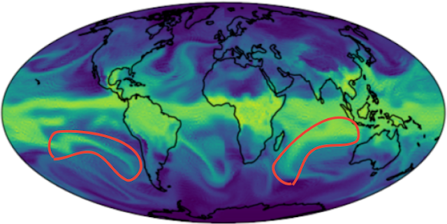
When projecting the sphere into a plane, the patch represented by the red circle is heavily distorted near the poles. This sampling problem hurts the accuracy of conventional CNNs and ViTs on spherical inputs.

Second, signals and local patterns on the sphere are often complicated by rotations, so models need a way to address that. We would like equivariance to 3D rotations, which ensures that learned features follow the rotations of the input. This leads to better utilization of the model parameters and allows training with less data. Equivariance to 3D rotations is also useful in most settings where inputs don’t have a preferred orientation, such as 3D shapes and molecules.
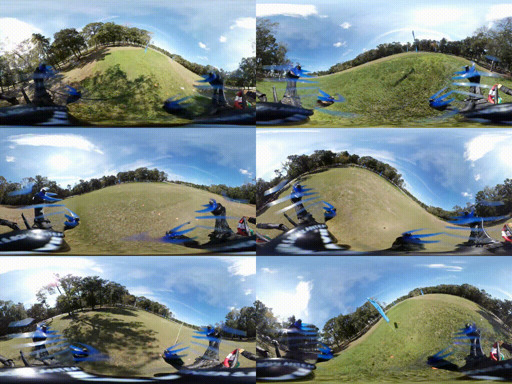
Drone racing with panoramic cameras. Here the sharp turns result in large 3D rotations of the spherical image. We would like our models to be robust to such rotations. Source: https://www.youtube.com/watch?v=_J7qXbbXY80 (licensed under CC BY)
In the atmosphere, it is common to see similar patterns appearing at different positions and orientations. We would like our models to share parameters to recognize these patterns.

With the above challenges in mind, in “Scaling Spherical CNNs”, presented at ICML 2023, we introduce an open-source library in JAX for deep learning on spherical surfaces. We demonstrate how applications of this library match or surpass state-of-the-art performance on weather forecasting and molecular property prediction benchmarks, tasks that are typically addressed with transformers and graph neural networks.


Background on spherical CNNs

Spherical CNNs solve both the problems of sampling and of robustness to rotation by leveraging spherical convolution and cross-correlation operations, which are typically computed via generalized Fourier transforms. For planar surfaces, however, convolution with small filters is faster, because it can be performed on regular grids without using Fourier transforms. The higher computational cost for spherical inputs has so far restricted the application of spherical CNNs to small models and datasets and low resolution datasets.


Our contributions

We have implemented the spherical convolutions from spin-weighted spherical CNNs in JAX with a focus on speed, and have enabled distributed training over a large number of TPUs using data parallelism. We also introduced a new phase collapse activation and spectral batch normalization layer, and a new residual block that improves accuracy and efficiency, which allows training more accurate models up to 100x larger than before. We apply these new models on molecular property regression and weather forecasting.
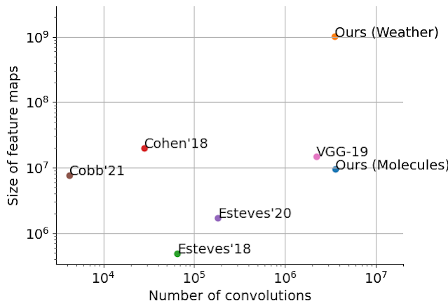
We scale spherical CNNs by up to two orders of magnitude in terms of feature sizes and model capacity, compared to the literature: Cohen’18Esteves’18Esteves’20, and Cobb’21VGG-19 is included as a conventional CNN reference. Our largest model for weather forecasting has 256 x 256 x 78 inputs and outputs, and runs 96 convolutional layers during training with a lowest internal resolution of 128 x 128 x 256.

Molecular property regression

Predicting properties of molecules has applications in drug discovery, where the goal is to quickly screen numerous molecules in search of those with desirable properties. Similar models may also be relevant in the design of drugs targeting the interaction between proteins. Current methods in computational or experimental quantum chemistry are expensive, which motivates the use of machine learning.

Molecules can be represented by a set of atoms and their positions in 3D space; rotations of the molecule change the positions but not the molecular properties. This motivates the application of spherical CNNs because of their rotation equivariance. However, molecules are not defined as signals on the sphere so the first step is to map them to a set of spherical functions. We do so by leveraging physics-based interactions between the atoms of the molecule.
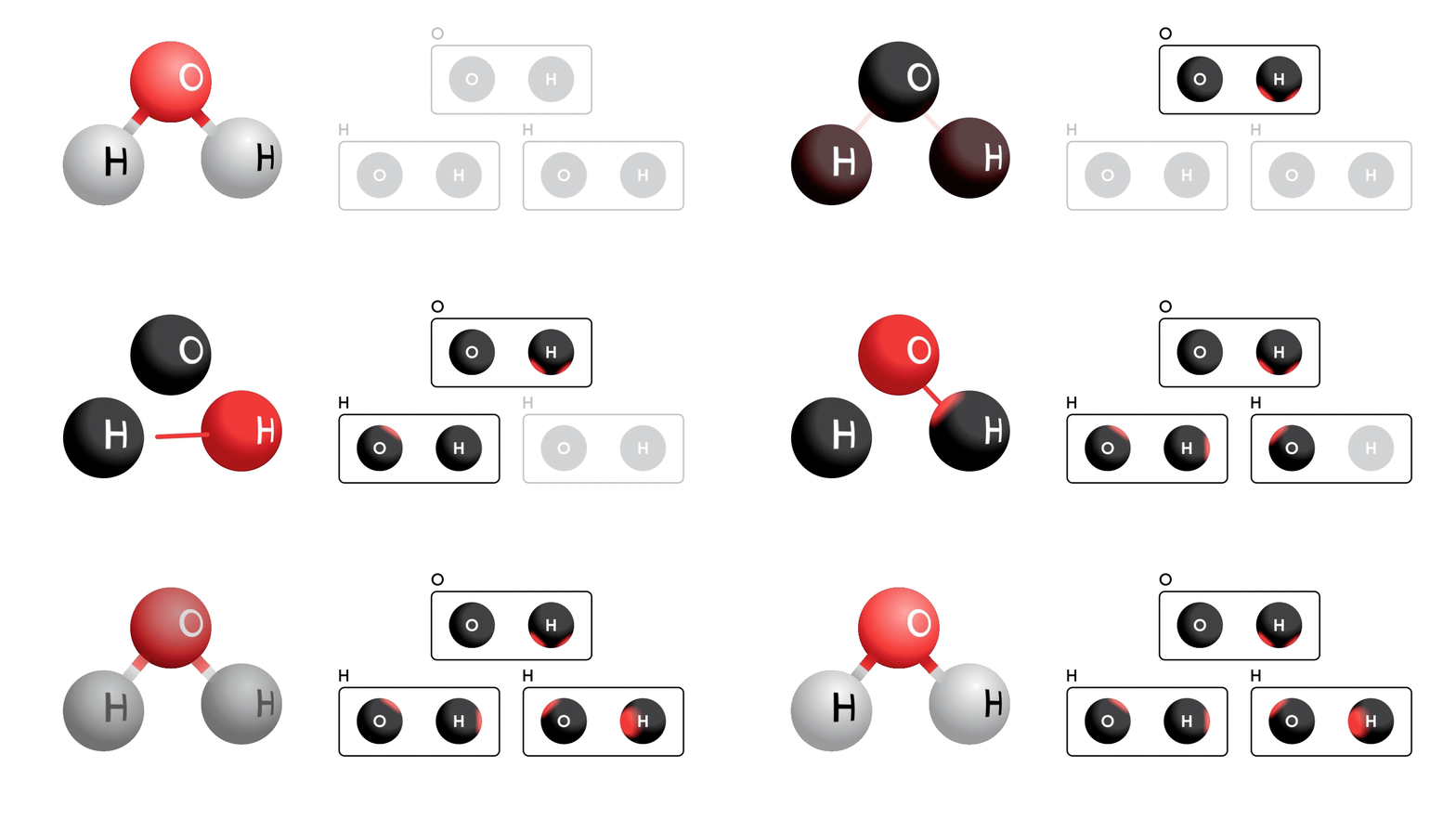
Each atom is represented by a set of spherical signals accumulating physical interactions with other atoms of each type (shown in the three panels on the right). For example, the oxygen atom (O; top panel) has a channel for oxygen (indicated by the sphere labeled “O” on the left) and hydrogen (“H”, right). The accumulated Coulomb forces on the oxygen atom with respect to the two hydrogen atoms is indicated by the red shaded regions on the bottom of the sphere labeled “H”. Because the oxygen atom contributes no forces to itself, the “O” sphere is uniform. We include extra channels for the Van der Waals forces.

Spherical CNNs are applied to each atom's features, and results are later combined to produce the property predictions. This results in state-of-the art performance in most properties as typically evaluated in the QM9 benchmark:
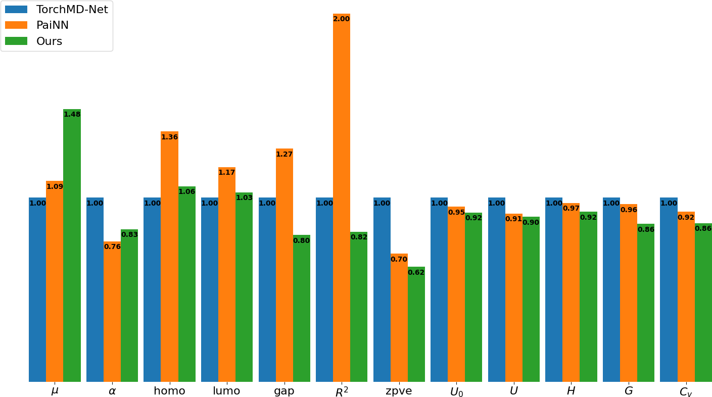
Error comparison against the state-of-the-art on 12 properties of QM9 (see the dataset paper for details). We show TorchMD-Net and PaiNN results, normalizing TorchMD-Net errors to 1.0 (lower is better). Our model, shown in green, outperforms the baselines in most targets.

Weather forecasting

Accurate climate forecasts serve as invaluable tools for providing timely warnings of extreme weather events, enabling effective water resource management, and guiding informed infrastructure planning. In a world increasingly threatened by climate disasters, there is an urgency to deliver forecasts much faster and more accurately over a longer time horizon than general circulation models. Forecasting models will also be important for predicting the safety and effectiveness of efforts intended to combat climate change, such as climate interventions. The current state-of-the-art uses costly numerical models based on fluid dynamics and thermodynamics, which tend to drift after a few days.

Given these challenges, there is an urgency for machine learning researchers to address climate forecasting problems, as data-driven techniques have the potential of both reducing the computational cost and improving long range accuracy. Spherical CNNs are suitable for this task since atmospheric data is natively presented on the sphere. They can also efficiently handle repeating patterns at different positions and orientations that are common in such data.

We apply our models to several weather forecasting benchmarks and outperform or match neural weather models based on conventional CNNs (specifically, 1, 2, and 3). Below we show results in a test setting where the model takes a number of atmospheric variables as input and predicts their values six hours ahead. The model is then iteratively applied on its own predictions to produce longer forecasts. During training, the model predicts up to three days ahead, and is evaluated up to five days. Keisler proposed a graph neural network for this task, but we show that spherical CNNs can match the GNN accuracy in the same setting.

Iterative weather forecasting up to five days (120h) ahead with spherical CNNs. The animations show the specific humidity forecast at a given pressure and its error.
Wind speed and temperature forecasts with spherical CNNs.

Additional resources

Our JAX library for efficient spherical CNNs is now available. We have shown applications to molecular property regression and weather forecasting, and we believe the library will be helpful in other scientific applications, as well as in computer vision and 3D vision.

Weather forecasting is an active area of research at Google with the goal of building more accurate and robust models — like Graphcast, a recent ML-based mid-range forecasting model — and to build tools that enable further advancement across the research community, such as the recently released WeatherBench 2.


Acknowledgements

This work was done in collaboration with Jean-Jacques Slotine, and is based on previous collaborations with Kostas Daniilidis and Christine Allen-Blanchette. We thank Stephan Hoyer, Stephan Rasp, and Ignacio Lopez-Gomez for helping with data processing and evaluation, and Fei Sha, Vivian Yang, Anudhyan Boral, Leonardo Zepeda-Núñez, and Avram Hershko for suggestions and discussions. We are thankful to Michael Riley and Corinna Cortes for supporting and encouraging this project.

Source: Google AI Blog


Re-weighted gradient descent via distributionally robust optimization

Deep neural networks (DNNs) have become essential for solving a wide range of tasks, from standard supervised learning (image classification using ViT) to meta-learning. The most commonly-used paradigm for learning DNNs is empirical risk minimization (ERM), which aims to identify a network that minimizes the average loss on training data points. Several algorithms, including stochastic gradient descent (SGD), Adam, and Adagrad, have been proposed for solving ERM. However, a drawback of ERM is that it weights all the samples equally, often ignoring the rare and more difficult samples, and focusing on the easier and abundant samples. This leads to suboptimal performance on unseen data, especially when the training data is scarce.

To overcome this challenge, recent works have developed data re-weighting techniques for improving ERM performance. However, these approaches focus on specific learning tasks (such as classification) and/or require learning an additional meta model that predicts the weights of each data point. The presence of an additional model significantly increases the complexity of training and makes them unwieldy in practice.

In “Stochastic Re-weighted Gradient Descent via Distributionally Robust Optimization” we introduce a variant of the classical SGD algorithm that re-weights data points during each optimization step based on their difficulty. Stochastic Re-weighted Gradient Descent (RGD) is a lightweight algorithm that comes with a simple closed-form expression, and can be applied to solve any learning task using just two lines of code. At any stage of the learning process, RGD simply reweights a data point as the exponential of its loss. We empirically demonstrate that the RGD reweighting algorithm improves the performance of numerous learning algorithms across various tasks, ranging from supervised learning to meta learning. Notably, we show improvements over state-of-the-art methods on DomainBed and Tabular classification. Moreover, the RGD algorithm also boosts performance for BERT using the GLUE benchmarks and ViT on ImageNet-1K.


Distributionally robust optimization

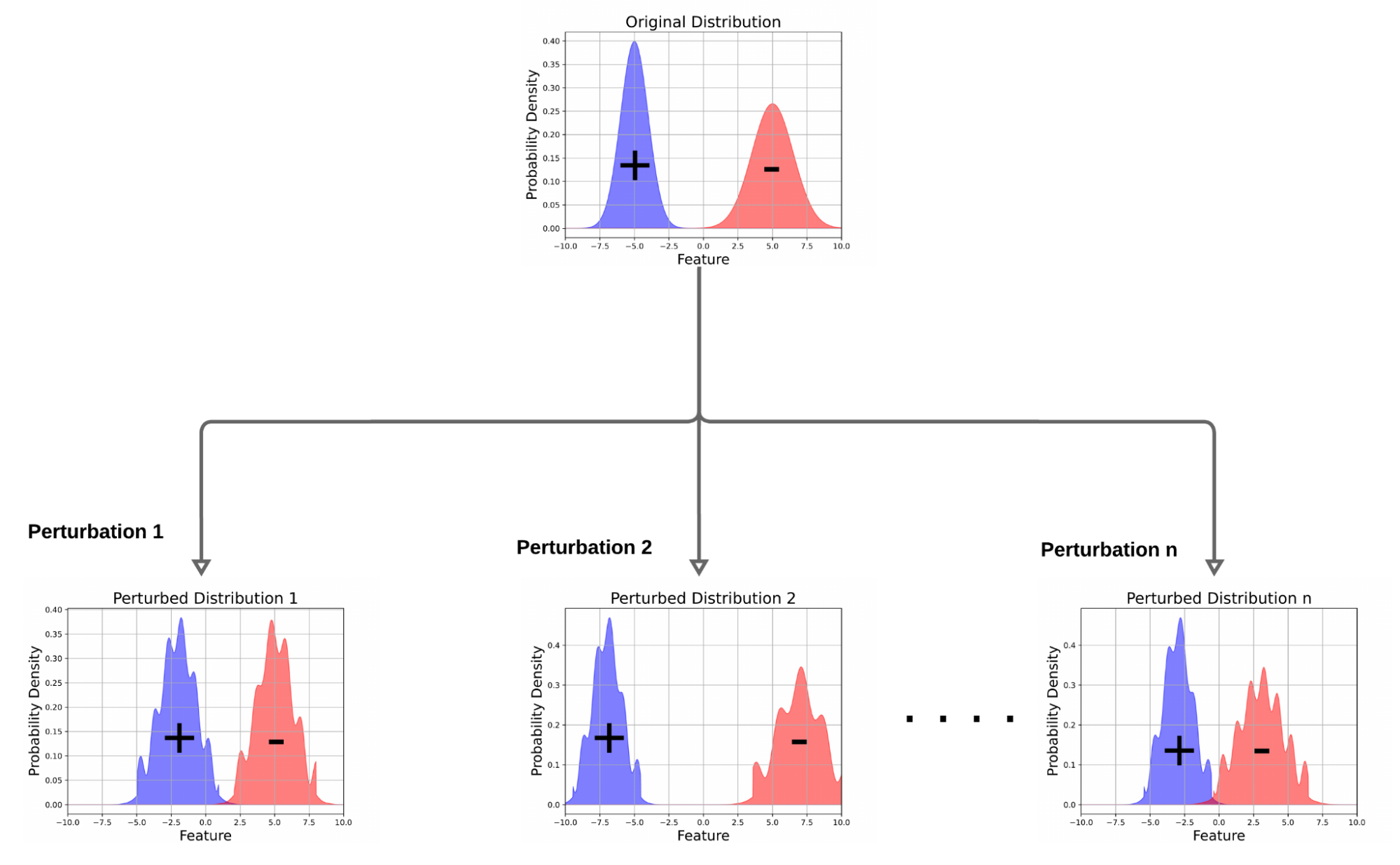
Distributionally robust optimization (DRO) is an approach that assumes a “worst-case” data distribution shift may occur, which can harm a model's performance. If a model has focussed on identifying few spurious features for prediction, these “worst-case” data distribution shifts could lead to the misclassification of samples and, thus, a performance drop. DRO optimizes the loss for samples in that “worst-case” distribution, making the model robust to perturbations (e.g., removing a small fraction of points from a dataset, minor up/down weighting of data points, etc.) in the data distribution. In the context of classification, this forces the model to place less emphasis on noisy features and more emphasis on useful and predictive features. Consequently, models optimized using DRO tend to have better generalization guarantees and stronger performance on unseen samples.

Inspired by these results, we develop the RGD algorithm as a technique for solving the DRO objective. Specifically, we focus on Kullback–Leibler divergence-based DRO, where one adds perturbations to create distributions that are close to the original data distribution in the KL divergence metric, enabling a model to perform well over all possible perturbations.

Figure illustrating DRO. In contrast to ERM, which learns a model that minimizes expected loss over original data distribution, DRO learns a model that performs well on several perturbed versions of the original data distribution.


Stochastic re-weighted gradient descent

Consider a random subset of samples (called a mini-batch), where each data point has an associated loss Li. Traditional algorithms like SGD give equal importance to all the samples in the mini-batch, and update the parameters of the model by descending along the averaged gradients of the loss of those samples. With RGD, we reweight each sample in the mini-batch and give more importance to points that the model identifies as more difficult. To be precise, we use the loss as a proxy to calculate the difficulty of a point, and reweight it by the exponential of its loss. Finally, we update the model parameters by descending along the weighted average of the gradients of the samples.

Due to stability considerations, in our experiments we clip and scale the loss before computing its exponential. Specifically, we clip the loss at some threshold T, and multiply it with a scalar that is inversely proportional to the threshold. An important aspect of RGD is its simplicity as it doesn’t rely on a meta model to compute the weights of data points. Furthermore, it can be implemented with two lines of code, and combined with any popular optimizers (such as SGD, Adam, and Adagrad.

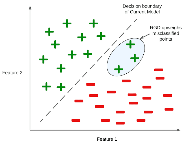
Figure illustrating the intuitive idea behind RGD in a binary classification setting. Feature 1 and Feature 2 are the features available to the model for predicting the label of a data point. RGD upweights the data points with high losses that have been misclassified by the model.


Results

We present empirical results comparing RGD with state-of-the-art techniques on standard supervised learning and domain adaptation (refer to the paper for results on meta learning). In all our experiments, we tune the clipping level and the learning rate of the optimizer using a held-out validation set.


Supervised learning

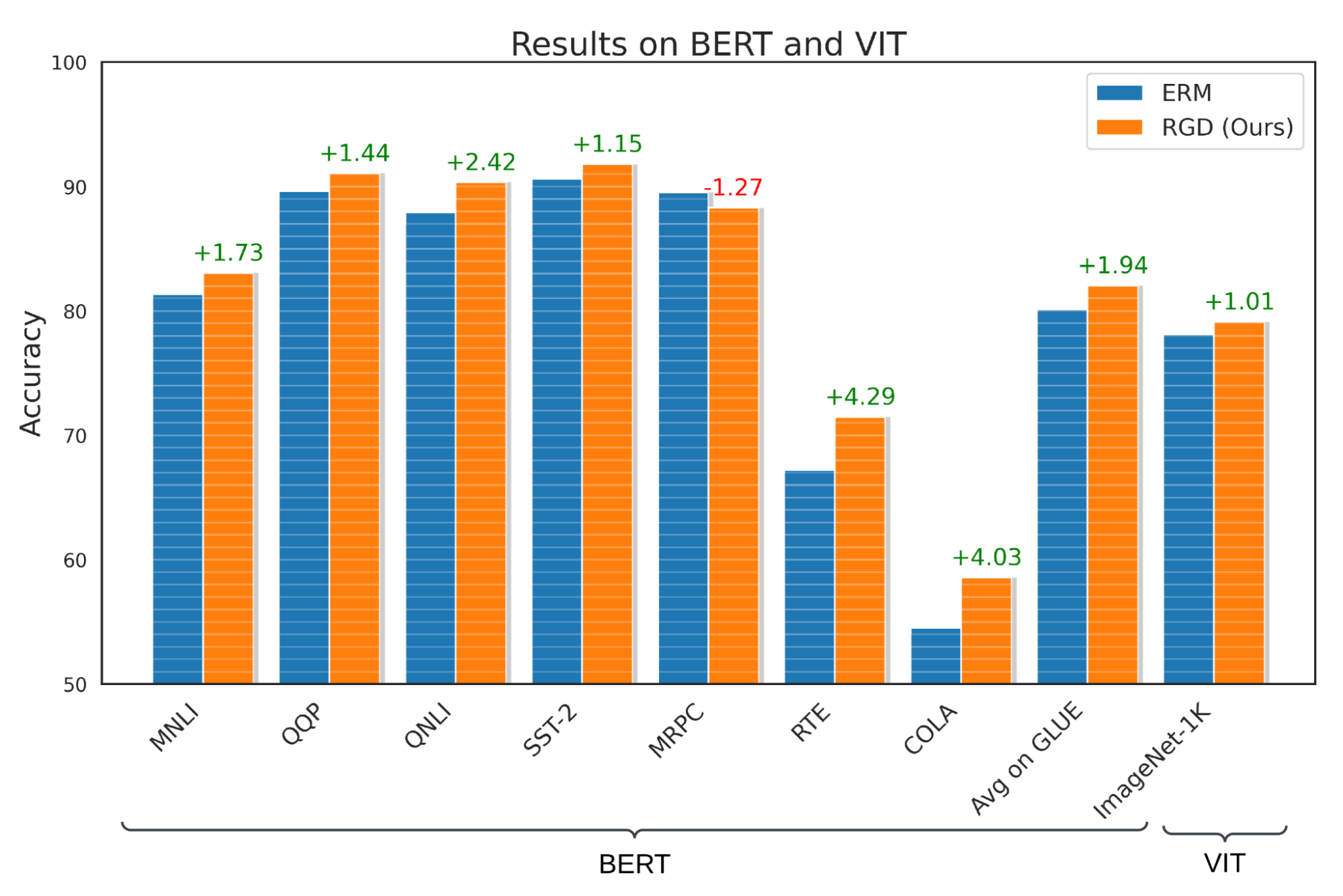
We evaluate RGD on several supervised learning tasks, including language, vision, and tabular classification. For the task of language classification, we apply RGD to the BERT model trained on the General Language Understanding Evaluation (GLUE) benchmark and show that RGD outperforms the BERT baseline by +1.94% with a standard deviation of 0.42%. To evaluate RGD’s performance on vision classification, we apply RGD to the ViT-S model trained on the ImageNet-1K dataset, and show that RGD outperforms the ViT-S baseline by +1.01% with a standard deviation of 0.23%. Moreover, we perform hypothesis tests to confirm that these results are statistically significant with a p-value that is less than 0.05.

RGD’s performance on language and vision classification using GLUE and Imagenet-1K benchmarks. Note that MNLI, QQP, QNLI, SST-2, MRPC, RTE and COLA are diverse datasets which comprise the GLUE benchmark.

For tabular classification, we use MET as our baseline, and consider various binary and multi-class datasets from UC Irvine's machine learning repository. We show that applying RGD to the MET framework improves its performance by 1.51% and 1.27% on binary and multi-class tabular classification, respectively, achieving state-of-the-art performance in this domain.


Performance of RGD for classification of various tabular datasets.


Domain generalization

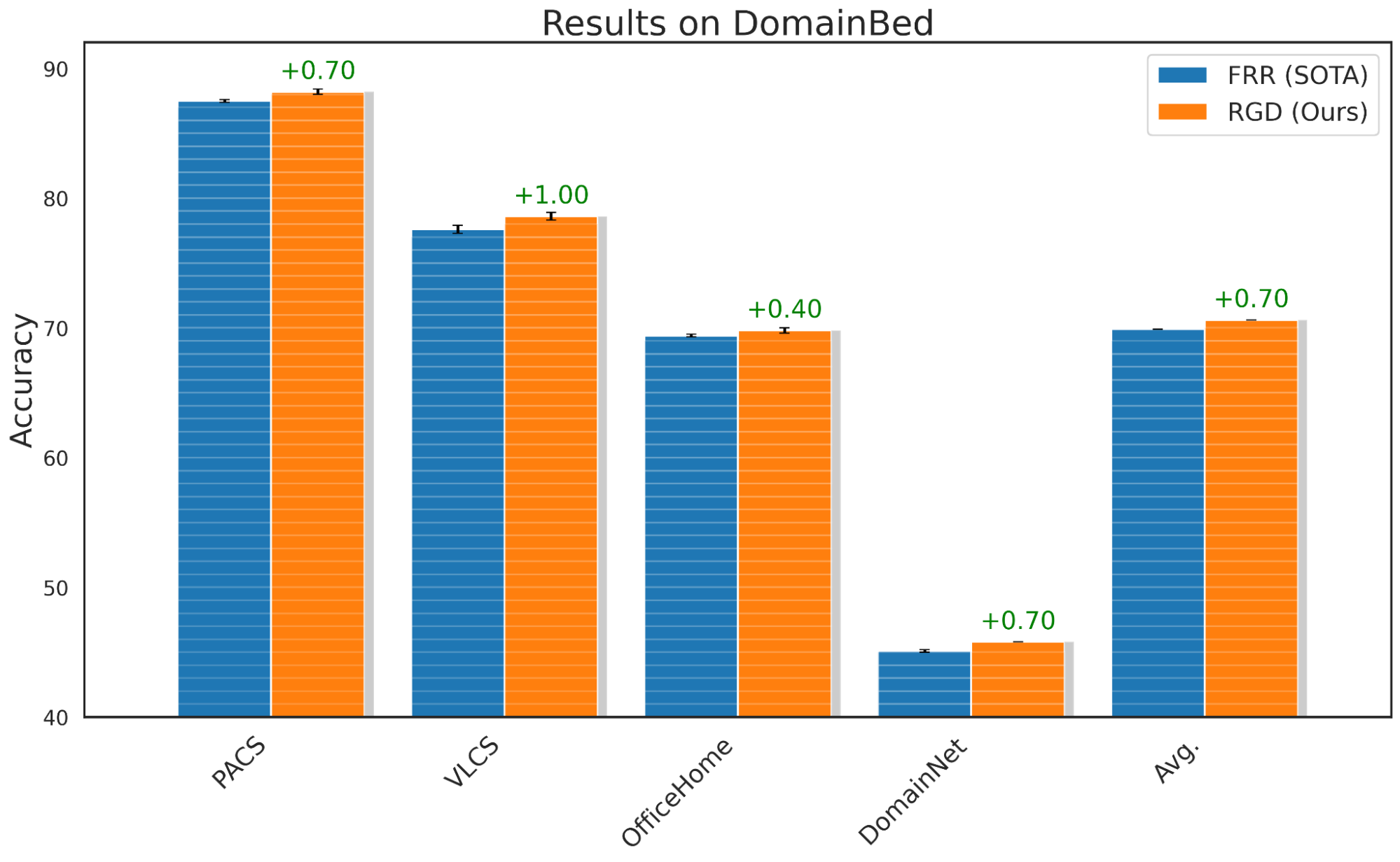
To evaluate RGD’s generalization capabilities, we use the standard DomainBed benchmark, which is commonly used to study a model’s out-of-domain performance. We apply RGD to FRR, a recent approach that improved out-of-domain benchmarks, and show that RGD with FRR performs an average of 0.7% better than the FRR baseline. Furthermore, we confirm with hypothesis tests that most benchmark results (except for Office Home) are statistically significant with a p-value less than 0.05.

Performance of RGD on DomainBed benchmark for distributional shifts.


Class imbalance and fairness

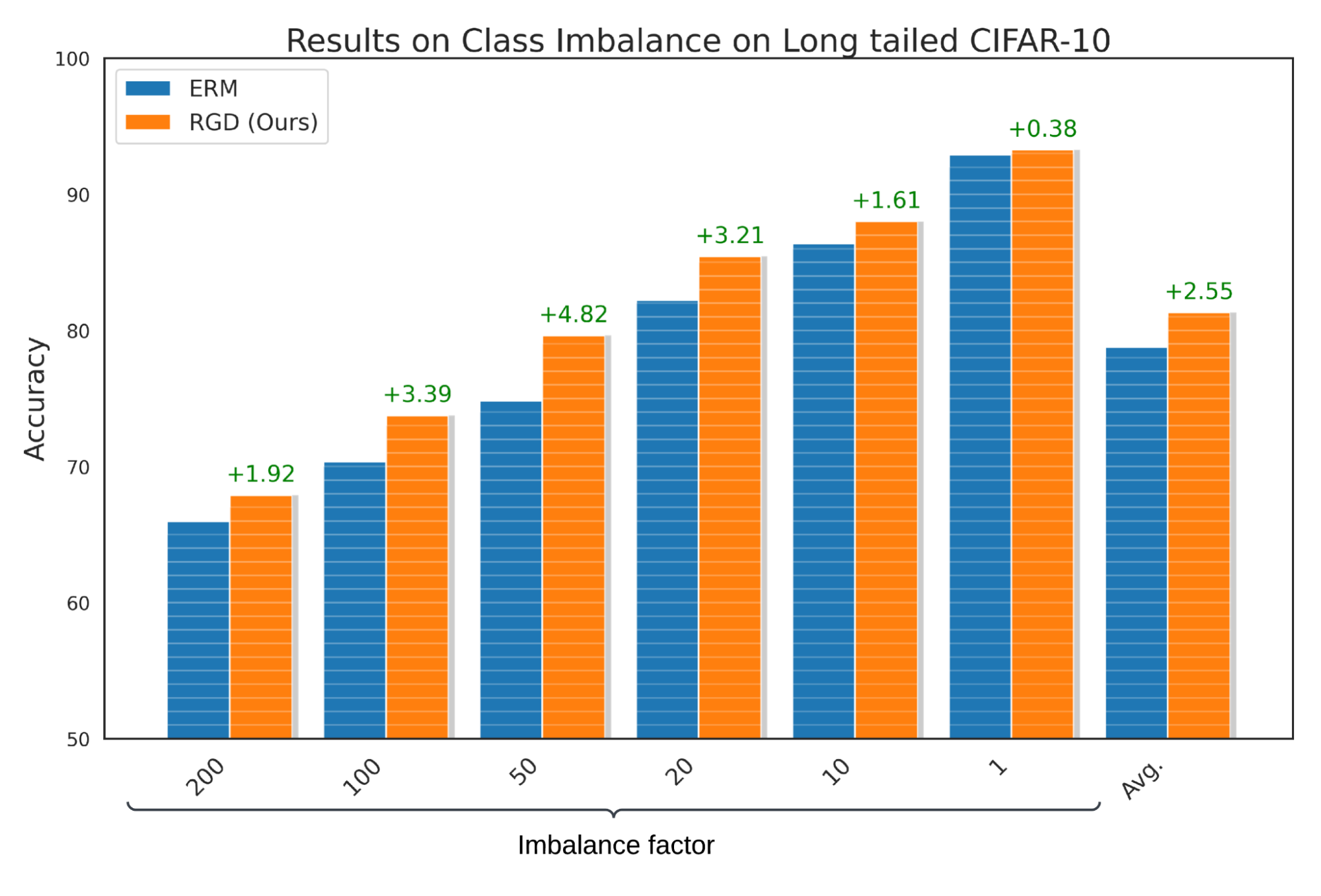
To demonstrate that models learned using RGD perform well despite class imbalance, where certain classes in the dataset are underrepresented, we compare RGD’s performance with ERM on long-tailed CIFAR-10. We report that RGD improves the accuracy of baseline ERM by an average of 2.55% with a standard deviation of 0.23%. Furthermore, we perform hypothesis tests and confirm that these results are statistically significant with a p-value of less than 0.05.

Performance of RGD on the long-tailed Cifar-10 benchmark for class imbalance domain.


Limitations

The RGD algorithm was developed using popular research datasets, which were already curated to remove corruptions (e.g., noise and incorrect labels). Therefore, RGD may not provide performance improvements in scenarios where training data has a high volume of corruptions. A potential approach to handle such scenarios is to apply an outlier removal technique to the RGD algorithm. This outlier removal technique should be capable of filtering out outliers from the mini-batch and sending the remaining points to our algorithm.


Conclusion

RGD has been shown to be effective on a variety of tasks, including out-of-domain generalization, tabular representation learning, and class imbalance. It is simple to implement and can be seamlessly integrated into existing algorithms with just two lines of code change. Overall, RGD is a promising technique for boosting the performance of DNNs, and could help push the boundaries in various domains.


Acknowledgements

The paper described in this blog post was written by Ramnath Kumar, Arun Sai Suggala, Dheeraj Nagaraj and Kushal Majmundar. We extend our sincere gratitude to the anonymous reviewers, Prateek Jain, Pradeep Shenoy, Anshul Nasery, Lovish Madaan, and the numerous dedicated members of the machine learning and optimization team at Google Research India for their invaluable feedback and contributions to this work.

Source: Google AI Blog


TSMixer: An all-MLP architecture for time series forecasting

Time series forecasting is critical to various real-world applications, from demand forecasting to pandemic spread prediction. In multivariate time series forecasting (forecasting multiple variants at the same time), one can split existing methods into two categories: univariate models and multivariate models. Univariate models focus on inter-series interactions or temporal patterns that encompass trends and seasonal patterns on a time series with a single variable. Examples of such trends and seasonal patterns might be the way mortgage rates increase due to inflation, and how traffic peaks during rush hour. In addition to inter-series patterns, multivariate models process intra-series features, known as cross-variate information, which is especially useful when one series is an advanced indicator of another series. For example, a rise in body weight may cause an increase in blood pressure, and increasing the price of a product may lead to a decrease in sales. Multivariate models have recently become popular solutions for multivariate forecasting as practitioners believe their capability of handling cross-variate information may lead to better performance.

In recent years, deep learning Transformer-based architectures have become a popular choice for multivariate forecasting models due to their superior performance on sequence tasks. However, advanced multivariate models perform surprisingly worse than simple univariate linear models on commonly-used long-term forecasting benchmarks, such as Electricity Transformer Temperature (ETT), Electricity, Traffic, and Weather. These results raise two questions:

  • Does cross-variate information benefit time series forecasting?
  • When cross-variate information is not beneficial, can multivariate models still perform as well as univariate models?

In “TSMixer: An All-MLP Architecture for Time Series Forecasting”, we analyze the advantages of univariate linear models and reveal their effectiveness. Insights from this analysis lead us to develop Time-Series Mixer (TSMixer), an advanced multivariate model that leverages linear model characteristics and performs well on long-term forecasting benchmarks. To the best of our knowledge, TSMixer is the first multivariate model that performs as well as state-of-the-art univariate models on long-term forecasting benchmarks, where we show that cross-variate information is less beneficial. To demonstrate the importance of cross-variate information, we evaluate a more challenging real-world application, M5. Finally, empirical results show that TSMixer outperforms state-of-the-art models, such as PatchTST, Fedformer, Autoformer, DeepAR and TFT.


TSMixer architecture

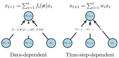
A key difference between linear models and Transformers is how they capture temporal patterns. On one hand, linear models apply fixed and time-step-dependent weights to capture static temporal patterns, and are unable to process cross-variate information. On the other hand, Transformers use attention mechanisms that apply dynamic and data-dependent weights at each time step, capturing dynamic temporal patterns and enabling them to process cross-variate information.

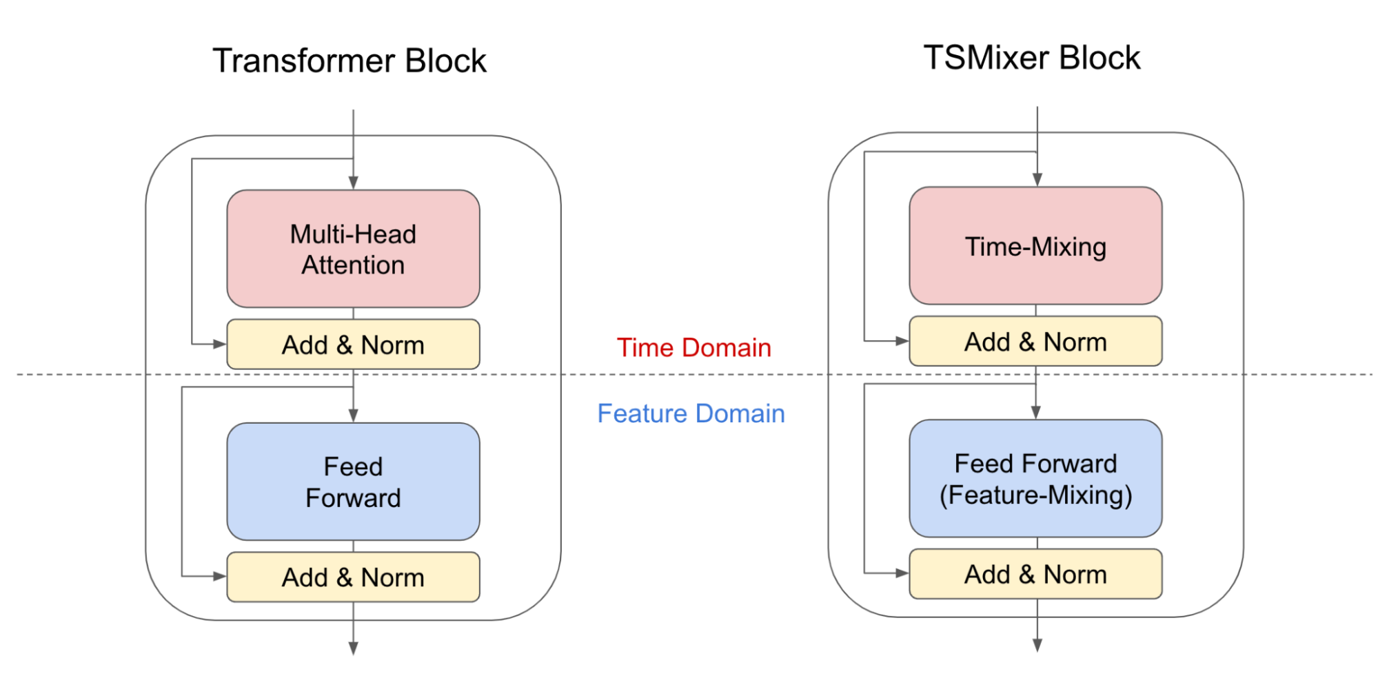
In our analysis, we show that under common assumptions of temporal patterns, linear models have naïve solutions to perfectly recover the time series or place bounds on the error, which means they are great solutions for learning static temporal patterns of univariate time series more effectively. In contrast, it is non-trivial to find similar solutions for attention mechanisms, as the weights applied to each time step are dynamic. Consequently, we develop a new architecture by replacing Transformer attention layers with linear layers. The resulting TSMixer model, which is similar to the computer vision MLP-Mixer method, alternates between applications of the multi-layer perceptron in different directions, which we call time-mixing and feature-mixing, respectively. The TSMixer architecture efficiently captures both temporal patterns and cross-variate information, as shown in the figure below. The residual designs ensure that TSMixer retains the capacity of temporal linear models while still being able to exploit cross-variate information.

Transformer block and TSMixer block architectures. TSMixer replaces the multi-head attention layer with time-mixing, a linear model applied on the time dimension.

Comparison between data-dependent (attention mechanisms) and time-step-dependent (linear models). This is an example of forecasting the next time step by learning the weights of the previous three time steps.


Evaluation on long-term forecasting benchmarks

We evaluate TSMixer using seven popular long-term forecasting datasets (ETTm1, ETTm2, ETTh1, ETTh2, Electricity, Traffic, and Weather), where recent research has shown that univariate linear models outperform advanced multivariate models with large margins. We compare TSMixer with state-of-the-art multivariate models (TFT, FEDformer, Autoformer, Informer), and univariate models, including linear models and PatchTST. The figure below shows the average improvement of mean squared error (MSE) by TSMixer compared with others. The average is calculated across datasets and multiple forecasting horizons. We demonstrate that TSMixer significantly outperforms other multivariate models and performs on par with state-of-the-art univariate models. These results show that multivariate models are capable of performing as well as univariate models.

The average MSE improvement of TSMixer compared with other baselines. The red bars show multivariate methods and the blue bars show univariate methods. TSMixer achieves significant improvement over other multivariate models and achieves comparable results to univariate models.


Ablation study

We performed an ablation study to compare TSMixer with TMix-Only, a TSMixer variant that consists of time mixing layers only. The results show that TMix-Only performs almost the same as TSMixer, which means the additional feature mixing layers do not improve the performance and confirms that cross-variate information is less beneficial on popular benchmarks. The results validate the superior univariate model performance shown in previous research. However, existing long-term forecasting benchmarks are not well representative of the need for cross-variate information in some real-world applications where time series may be intermittent or sparse, hence temporal patterns may not be sufficient for forecasting. Therefore, it may be inappropriate to evaluate multivariate forecasting models solely on these benchmarks.


Evaluation on M5: Effectiveness of cross-variate information

To further demonstrate the benefit of multivariate models, we evaluate TSMixer on the challenging M5 benchmark, a large-scale retail dataset containing crucial cross-variate interactions. M5 contains the information of 30,490 products collected over 5 years. Each product description includes time series data, like daily sales, sell price, promotional event information, and static (non-time-series) features, such as store location and product category. The goal is to forecast the daily sales of each product for the next 28 days, evaluated using the weighted root mean square scaled error (WRMSSE) from the M5 competition. The complicated nature of retail makes it more challenging to forecast solely using univariate models that focus on temporal patterns, so multivariate models with cross-variate information and even auxiliary features are more essential.

First, we compare TSMixer to other methods only considering the historical data, such as daily sales and historical sell prices. The results show that multivariate models outperforms univariate models significantly, indicating the usefulness of cross-variate information. And among all compared methods, TSMixer effectively leverages the cross-variate information and achieves the best performance.

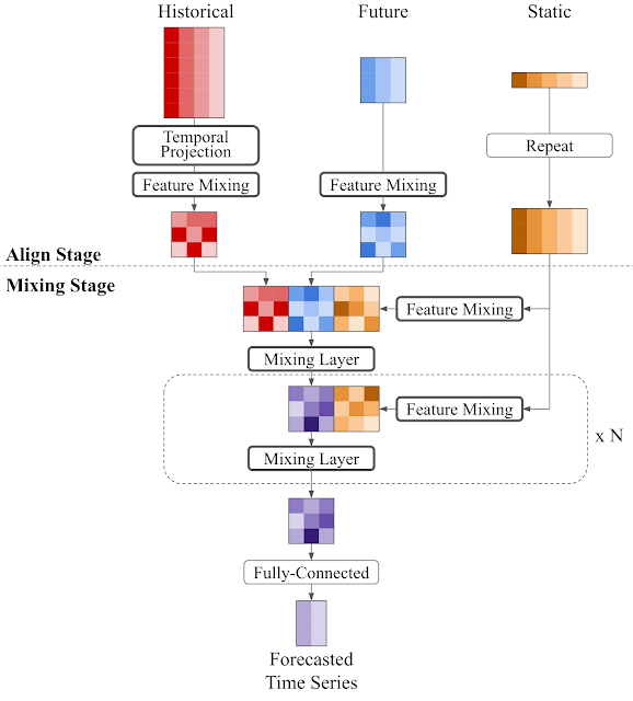
Additionally, to leverage more information, such as static features (e.g., store location, product category) and future time series (e.g., a promotional event scheduled in coming days) provided in M5, we propose a principle design to extend TSMixer. The extended TSMixer aligns different types of features into the same length, and then applies multiple mixing layers to the concatenated features to make predictions. The extended TSMixer architecture outperforms models popular in industrial applications, including DeepAR and TFT, showcasing its strong potential for real-world impact.

The architecture of the extended TSMixer. In the first stage (align stage), it aligns the different types of features into the same length before concatenating them. In the second stage (mixing stage) it applies multiple mixing layers conditioned with static features.

The WRMSSE on M5. The first three methods (blue) are univariate models. The middle three methods (orange) are multivariate models that consider only historical features. The last three methods (red) are multivariate models that consider historical, future, and static features.


Conclusion

We present TSMixer, an advanced multivariate model that leverages linear model characteristics and performs as well as state-of-the-art univariate models on long-term forecasting benchmarks. TSMixer creates new possibilities for the development of time series forecasting architectures by providing insights into the importance of cross-variate and auxiliary information in real-world scenarios. The empirical results highlight the need to consider more realistic benchmarks for multivariate forecasting models in future research. We hope that this work will inspire further exploration in the field of time series forecasting, and lead to the development of more powerful and effective models that can be applied to real-world applications.


Acknowledgements

This research was conducted by Si-An Chen, Chun-Liang Li, Nate Yoder, Sercan O. Arik, and Tomas Pfister.

Source: Google AI Blog


Language to rewards for robotic skill synthesis

Empowering end-users to interactively teach robots to perform novel tasks is a crucial capability for their successful integration into real-world applications. For example, a user may want to teach a robot dog to perform a new trick, or teach a manipulator robot how to organize a lunch box based on user preferences. The recent advancements in large language models (LLMs) pre-trained on extensive internet data have shown a promising path towards achieving this goal. Indeed, researchers have explored diverse ways of leveraging LLMs for robotics, from step-by-step planning and goal-oriented dialogue to robot-code-writing agents.

While these methods impart new modes of compositional generalization, they focus on using language to link together new behaviors from an existing library of control primitives that are either manually engineered or learned a priori. Despite having internal knowledge about robot motions, LLMs struggle to directly output low-level robot commands due to the limited availability of relevant training data. As a result, the expression of these methods are bottlenecked by the breadth of the available primitives, the design of which often requires extensive expert knowledge or massive data collection.

In “Language to Rewards for Robotic Skill Synthesis”, we propose an approach to enable users to teach robots novel actions through natural language input. To do so, we leverage reward functions as an interface that bridges the gap between language and low-level robot actions. We posit that reward functions provide an ideal interface for such tasks given their richness in semantics, modularity, and interpretability. They also provide a direct connection to low-level policies through black-box optimization or reinforcement learning (RL). We developed a language-to-reward system that leverages LLMs to translate natural language user instructions into reward-specifying code and then applies MuJoCo MPC to find optimal low-level robot actions that maximize the generated reward function. We demonstrate our language-to-reward system on a variety of robotic control tasks in simulation using a quadruped robot and a dexterous manipulator robot. We further validate our method on a physical robot manipulator.

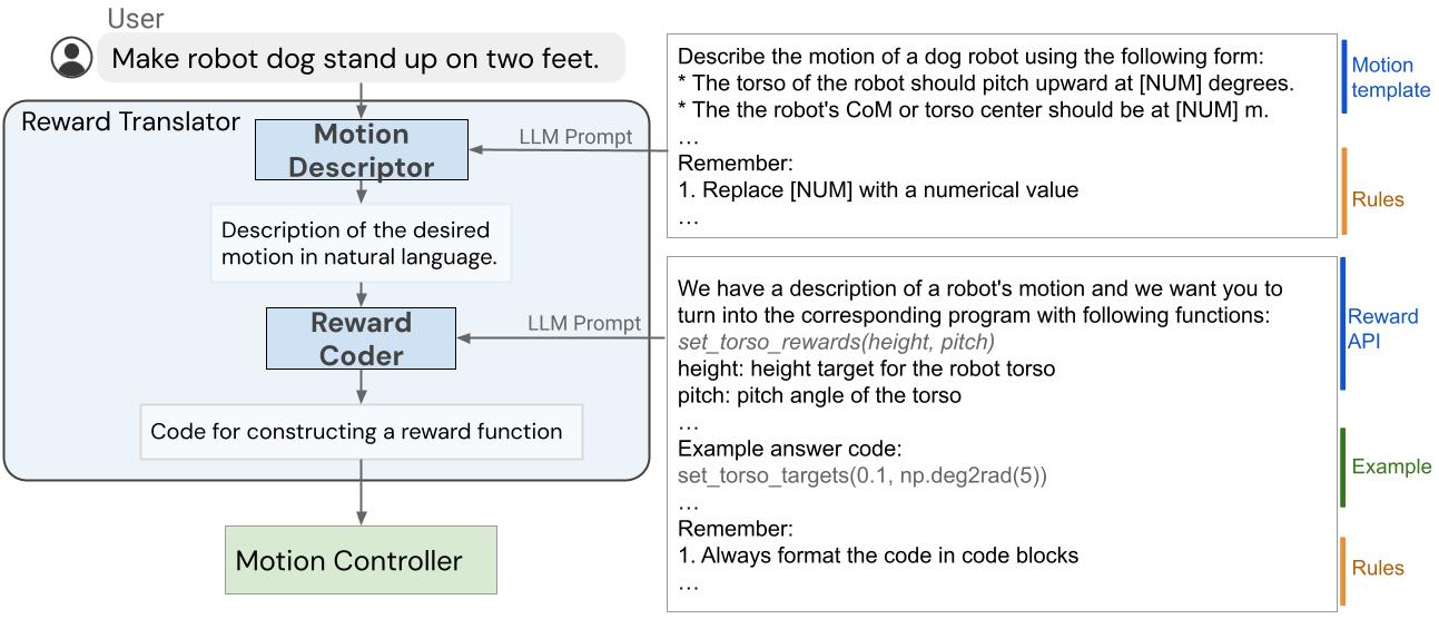
The language-to-reward system consists of two core components: (1) a Reward Translator, and (2) a Motion Controller. The Reward Translator maps natural language instruction from users to reward functions represented as python code. The Motion Controller optimizes the given reward function using receding horizon optimization to find the optimal low-level robot actions, such as the amount of torque that should be applied to each robot motor.

LLMs cannot directly generate low-level robotic actions due to lack of data in pre-training dataset. We propose to use reward functions to bridge the gap between language and low-level robot actions, and enable novel complex robot motions from natural language instructions.


Reward Translator: Translating user instructions to reward functions

The Reward Translator module was built with the goal of mapping natural language user instructions to reward functions. Reward tuning is highly domain-specific and requires expert knowledge, so it was not surprising to us when we found that LLMs trained on generic language datasets are unable to directly generate a reward function for a specific hardware. To address this, we apply the in-context learning ability of LLMs. Furthermore, we split the Reward Translator into two sub-modules: Motion Descriptor and Reward Coder.


Motion Descriptor

First, we design a Motion Descriptor that interprets input from a user and expands it into a natural language description of the desired robot motion following a predefined template. This Motion Descriptor turns potentially ambiguous or vague user instructions into more specific and descriptive robot motions, making the reward coding task more stable. Moreover, users interact with the system through the motion description field, so this also provides a more interpretable interface for users compared to directly showing the reward function.

To create the Motion Descriptor, we use an LLM to translate the user input into a detailed description of the desired robot motion. We design prompts that guide the LLMs to output the motion description with the right amount of details and format. By translating a vague user instruction into a more detailed description, we are able to more reliably generate the reward function with our system. This idea can also be potentially applied more generally beyond robotics tasks, and is relevant to Inner-Monologue and chain-of-thought prompting.


Reward Coder

In the second stage, we use the same LLM from Motion Descriptor for Reward Coder, which translates generated motion description into the reward function. Reward functions are represented using python code to benefit from the LLMs’ knowledge of reward, coding, and code structure.

Ideally, we would like to use an LLM to directly generate a reward function R (s, t) that maps the robot state s and time t into a scalar reward value. However, generating the correct reward function from scratch is still a challenging problem for LLMs and correcting the errors requires the user to understand the generated code to provide the right feedback. As such, we pre-define a set of reward terms that are commonly used for the robot of interest and allow LLMs to composite different reward terms to formulate the final reward function. To achieve this, we design a prompt that specifies the reward terms and guide the LLM to generate the correct reward function for the task.

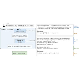
The internal structure of the Reward Translator, which is tasked to map user inputs to reward functions.


Motion Controller: Translating reward functions to robot actions

The Motion Controller takes the reward function generated by the Reward Translator and synthesizes a controller that maps robot observation to low-level robot actions. To do this, we formulate the controller synthesis problem as a Markov decision process (MDP), which can be solved using different strategies, including RL, offline trajectory optimization, or model predictive control (MPC). Specifically, we use an open-source implementation based on the MuJoCo MPC (MJPC).

MJPC has demonstrated the interactive creation of diverse behaviors, such as legged locomotion, grasping, and finger-gaiting, while supporting multiple planning algorithms, such as iterative linear–quadratic–Gaussian (iLQG) and predictive sampling. More importantly, the frequent re-planning in MJPC empowers its robustness to uncertainties in the system and enables an interactive motion synthesis and correction system when combined with LLMs.


Examples


Robot dog

In the first example, we apply the language-to-reward system to a simulated quadruped robot and teach it to perform various skills. For each skill, the user will provide a concise instruction to the system, which will then synthesize the robot motion by using reward functions as an intermediate interface.


Dexterous manipulator

We then apply the language-to-reward system to a dexterous manipulator robot to perform a variety of manipulation tasks. The dexterous manipulator has 27 degrees of freedom, which is very challenging to control. Many of these tasks require manipulation skills beyond grasping, making it difficult for pre-designed primitives to work. We also include an example where the user can interactively instruct the robot to place an apple inside a drawer.


Validation on real robots

We also validate the language-to-reward method using a real-world manipulation robot to perform tasks such as picking up objects and opening a drawer. To perform the optimization in Motion Controller, we use AprilTag, a fiducial marker system, and F-VLM, an open-vocabulary object detection tool, to identify the position of the table and objects being manipulated.


Conclusion

In this work, we describe a new paradigm for interfacing an LLM with a robot through reward functions, powered by a low-level model predictive control tool, MuJoCo MPC. Using reward functions as the interface enables LLMs to work in a semantic-rich space that plays to the strengths of LLMs, while ensuring the expressiveness of the resulting controller. To further improve the performance of the system, we propose to use a structured motion description template to better extract internal knowledge about robot motions from LLMs. We demonstrate our proposed system on two simulated robot platforms and one real robot for both locomotion and manipulation tasks.


Acknowledgements

We would like to thank our co-authors Nimrod Gileadi, Chuyuan Fu, Sean Kirmani, Kuang-Huei Lee, Montse Gonzalez Arenas, Hao-Tien Lewis Chiang, Tom Erez, Leonard Hasenclever, Brian Ichter, Ted Xiao, Peng Xu, Andy Zeng, Tingnan Zhang, Nicolas Heess, Dorsa Sadigh, Jie Tan, and Yuval Tassa for their help and support in various aspects of the project. We would also like to acknowledge Ken Caluwaerts, Kristian Hartikainen, Steven Bohez, Carolina Parada, Marc Toussaint, and the greater teams at Google DeepMind for their feedback and contributions.

Source: Google AI Blog


STUDY: Socially aware temporally causal decoder recommender systems

Reading has many benefits for young students, such as better linguistic and life skills, and reading for pleasure has been shown to correlate with academic success. Furthermore students have reported improved emotional wellbeing from reading, as well as better general knowledge and better understanding of other cultures. With the vast amount of reading material both online and off, finding age-appropriate, relevant and engaging content can be a challenging task, but helping students do so is a necessary step to engage them in reading. Effective recommendations that present students with relevant reading material helps keep students reading, and this is where machine learning (ML) can help.

ML has been widely used in building recommender systems for various types of digital content, ranging from videos to books to e-commerce items. Recommender systems are used across a range of digital platforms to help surface relevant and engaging content to users. In these systems, ML models are trained to suggest items to each user individually based on user preferences, user engagement, and the items under recommendation. These data provide a strong learning signal for models to be able to recommend items that are likely to be of interest, thereby improving user experience.

In “STUDY: Socially Aware Temporally Causal Decoder Recommender Systems”, we present a content recommender system for audiobooks in an educational setting taking into account the social nature of reading. We developed the STUDY algorithm in partnership with Learning Ally, an educational nonprofit, aimed at promoting reading in dyslexic students, that provides audiobooks to students through a school-wide subscription program. Leveraging the wide range of audiobooks in the Learning Ally library, our goal is to help students find the right content to help boost their reading experience and engagement. Motivated by the fact that what a person’s peers are currently reading has significant effects on what they would find interesting to read, we jointly process the reading engagement history of students who are in the same classroom. This allows our model to benefit from live information about what is currently trending within the student’s localized social group, in this case, their classroom.


Data

Learning Ally has a large digital library of curated audiobooks targeted at students, making it well-suited for building a social recommendation model to help improve student learning outcomes. We received two years of anonymized audiobook consumption data. All students, schools and groupings in the data were anonymized, only identified by a randomly generated ID not traceable back to real entities by Google. Furthermore all potentially identifiable metadata was only shared in an aggregated form, to protect students and institutions from being re-identified. The data consisted of time-stamped records of student’s interactions with audiobooks. For each interaction we have an anonymized student ID (which includes the student’s grade level and anonymized school ID), an audiobook identifier and a date. While many schools distribute students in a single grade across several classrooms, we leverage this metadata to make the simplifying assumption that all students in the same school and in the same grade level are in the same classroom. While this provides the foundation needed to build a better social recommender model, it's important to note that this does not enable us to re-identify individuals, class groups or schools.


The STUDY algorithm

We framed the recommendation problem as a click-through rate prediction problem, where we model the conditional probability of a user interacting with each specific item conditioned on both 1) user and item characteristics and 2) the item interaction history sequence for the user at hand. Previous work suggests Transformer-based models, a widely used model class developed by Google Research, are well suited for modeling this problem. When each user is processed individually this becomes an autoregressive sequence modeling problem. We use this conceptual framework to model our data and then extend this framework to create the STUDY approach.

While this approach for click-through rate prediction can model dependencies between past and future item preferences for an individual user and can learn patterns of similarity across users at train time, it cannot model dependencies across different users at inference time. To recognise the social nature of reading and remediate this shortcoming we developed the STUDY model, which concatenates multiple sequences of books read by each student into a single sequence that collects data from multiple students in a single classroom.

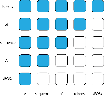
However, this data representation requires careful diligence if it is to be modeled by transformers. In transformers, the attention mask is the matrix that controls which inputs can be used to inform the predictions of which outputs. The pattern of using all prior tokens in a sequence to inform the prediction of an output leads to the upper triangular attention matrix traditionally found in causal decoders. However, since the sequence fed into the STUDY model is not temporally ordered, even though each of its constituent subsequences is, a standard causal decoder is no longer a good fit for this sequence. When trying to predict each token, the model is not allowed to attend to every token that precedes it in the sequence; some of these tokens might have timestamps that are later and contain information that would not be available at deployment time.

In this figure we show the attention mask typically used in causal decoders. Each column represents an output and each column represents an output. A value of 1 (shown as blue) for a matrix entry at a particular position denotes that the model can observe the input of that row when predicting the output of the corresponding column, whereas a value of 0 (shown as white) denotes the opposite.

The STUDY model builds on causal transformers by replacing the triangular matrix attention mask with a flexible attention mask with values based on timestamps to allow attention across different subsequences. Compared to a regular transformer, which would not allow attention across different subsequences and would have a triangular matrix mask within sequence, STUDY maintains a causal triangular attention matrix within a sequence and has flexible values across sequences with values that depend on timestamps. Hence, predictions at any output point in the sequence are informed by all input points that occurred in the past relative to the current time point, regardless of whether they appear before or after the current input in the sequence. This causal constraint is important because if it is not enforced at train time, the model could potentially learn to make predictions using information from the future, which would not be available for a real world deployment.

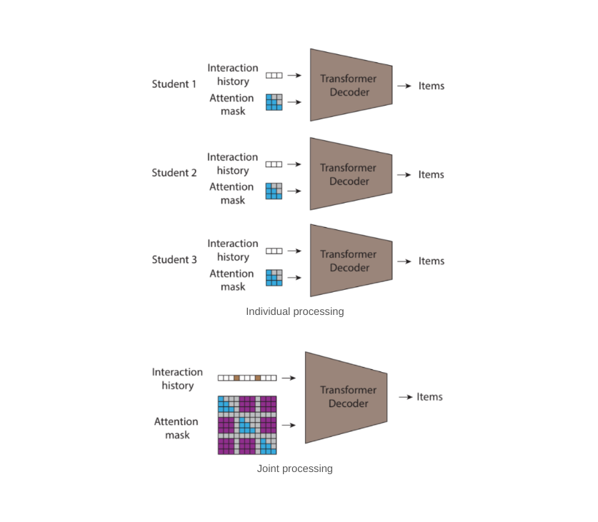
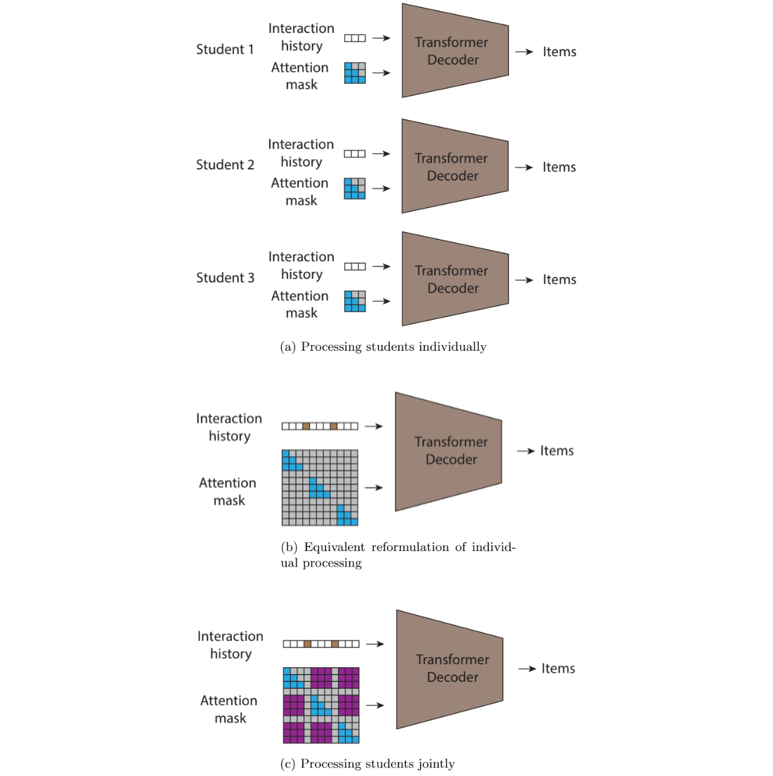
In (a) we show a sequential autoregressive transformer with causal attention that processes each user individually; in (b) we show an equivalent joint forward pass that results in the same computation as (a); and finally, in (c) we show that by introducing new nonzero values (shown in purple) to the attention mask we allow information to flow across users. We do this by allowing a prediction to condition on all interactions with an earlier timestamp, irrespective of whether the interaction came from the same user or not.

Experiments

We used the Learning Ally dataset to train the STUDY model along with multiple baselines for comparison. We implemented an autoregressive click-through rate transformer decoder, which we refer to as “Individual”, a k-nearest neighbor baseline (KNN), and a comparable social baseline, social attention memory network (SAMN). We used the data from the first school year for training and we used the data from the second school year for validation and testing.

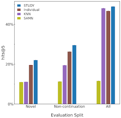
We evaluated these models by measuring the percentage of the time the next item the user actually interacted with was in the model’s top n recommendations, i.e., hits@n, for different values of n. In addition to evaluating the models on the entire test set we also report the models’ scores on two subsets of the test set that are more challenging than the whole data set. We observed that students will typically interact with an audiobook over multiple sessions, so simply recommending the last book read by the user would be a strong trivial recommendation. Hence, the first test subset, which we refer to as “non-continuation”, is where we only look at each model’s performance on recommendations when the students interact with books that are different from the previous interaction. We also observe that students revisit books they have read in the past, so strong performance on the test set can be achieved by restricting the recommendations made for each student to only the books they have read in the past. Although there might be value in recommending old favorites to students, much value from recommender systems comes from surfacing content that is new and unknown to the user. To measure this we evaluate the models on the subset of the test set where the students interact with a title for the first time. We name this evaluation subset “novel”.

We find that STUDY outperforms all other tested models across almost every single slice we evaluated against.

In this figure we compare the performance of four models, Study, Individual, KNN and SAMN. We measure the performance with hits@5, i.e., how likely the model is to suggest the next title the user read within the model’s top 5 recommendations. We evaluate the model on the entire test set (all) as well as the novel and non-continuation splits. We see STUDY consistently outperforms the other three models presented across all splits.

Importance of appropriate grouping

At the heart of the STUDY algorithm is organizing users into groups and doing joint inference over multiple users who are in the same group in a single forward pass of the model. We conducted an ablation study where we looked at the importance of the actual groupings used on the performance of the model. In our presented model we group together all students who are in the same grade level and school. We then experiment with groups defined by all students in the same grade level and district and also place all students in a single group with a random subset used for each forward pass. We also compare these models against the Individual model for reference.

We found that using groups that were more localized was more effective, with the school and grade level grouping outperforming the district and grade level grouping. This supports the hypothesis that the STUDY model is successful because of the social nature of activities such as reading — people’s reading choices are likely to correlate with the reading choices of those around them. Both of these models outperformed the other two models (single group and Individual) where grade level is not used to group students. This suggests that data from users with similar reading levels and interests is beneficial for performance.


Future work

This work is limited to modeling recommendations for user populations where the social connections are assumed to be homogenous. In the future it would be beneficial to model a user population where relationships are not homogeneous, i.e., where categorically different types of relationships exist or where the relative strength or influence of different relationships is known.


Acknowledgements

This work involved collaborative efforts from a multidisciplinary team of researchers, software engineers and educational subject matter experts. We thank our co-authors: Diana Mincu, Lauren Harrell, and Katherine Heller from Google. We also thank our colleagues at Learning Ally, Jeff Ho, Akshat Shah, Erin Walker, and Tyler Bastian, and our collaborators at Google, Marc Repnyek, Aki Estrella, Fernando Diaz, Scott Sanner, Emily Salkey and Lev Proleev.

Source: Google AI Blog


AdaTape: Foundation model with adaptive computation and dynamic read-and-write

Adaptive computation refers to the ability of a machine learning system to adjust its behavior in response to changes in the environment. While conventional neural networks have a fixed function and computation capacity, i.e., they spend the same number of FLOPs for processing different inputs, a model with adaptive and dynamic computation modulates the computational budget it dedicates to processing each input, depending on the complexity of the input.

Adaptive computation in neural networks is appealing for two key reasons. First, the mechanism that introduces adaptivity provides an inductive bias that can play a key role in solving some challenging tasks. For instance, enabling different numbers of computational steps for different inputs can be crucial in solving arithmetic problems that require modeling hierarchies of different depths. Second, it gives practitioners the ability to tune the cost of inference through greater flexibility offered by dynamic computation, as these models can be adjusted to spend more FLOPs processing a new input.

Neural networks can be made adaptive by using different functions or computation budgets for various inputs. A deep neural network can be thought of as a function that outputs a result based on both the input and its parameters. To implement adaptive function types, a subset of parameters are selectively activated based on the input, a process referred to as conditional computation. Adaptivity based on the function type has been explored in studies on mixture-of-experts, where the sparsely activated parameters for each input sample are determined through routing.

Another area of research in adaptive computation involves dynamic computation budgets. Unlike in standard neural networks, such as T5, GPT-3, PaLM, and ViT, whose computation budget is fixed for different samples, recent research has demonstrated that adaptive computation budgets can improve performance on tasks where transformers fall short. Many of these works achieve adaptivity by using dynamic depth to allocate the computation budget. For example, the Adaptive Computation Time (ACT) algorithm was proposed to provide an adaptive computational budget for recurrent neural networks. The Universal Transformer extends the ACT algorithm to transformers by making the computation budget dependent on the number of transformer layers used for each input example or token. Recent studies, like PonderNet, follow a similar approach while improving the dynamic halting mechanisms.

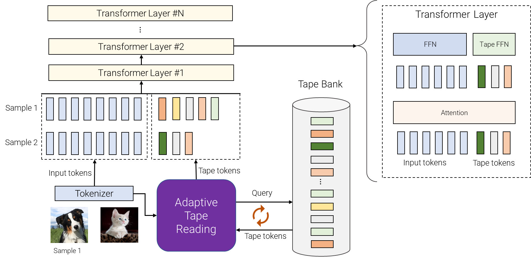
In the paper “Adaptive Computation with Elastic Input Sequence”, we introduce a new model that utilizes adaptive computation, called AdaTape. This model is a Transformer-based architecture that uses a dynamic set of tokens to create elastic input sequences, providing a unique perspective on adaptivity in comparison to previous works. AdaTape uses an adaptive tape reading mechanism to determine a varying number of tape tokens that are added to each input based on input’s complexity. AdaTape is very simple to implement, provides an effective knob to increase the accuracy when needed, but is also much more efficient compared to other adaptive baselines because it directly injects adaptivity into the input sequence instead of the model depth. Finally, Adatape offers better performance on standard tasks, like image classification, as well as algorithmic tasks, while maintaining a favorable quality and cost tradeoff.


Adaptive computation transformer with elastic input sequence

AdaTape uses both the adaptive function types and a dynamic computation budget. Specifically, for a batch of input sequences after tokenization (e.g., a linear projection of non-overlapping patches from an image in the vision transformer), AdaTape uses a vector representing each input to dynamically select a variable-sized sequence of tape tokens.

AdaTape uses a bank of tokens, called a “tape bank”, to store all the candidate tape tokens that interact with the model through the adaptive tape reading mechanism. We explore two different methods for creating the tape bank: an input-driven bank and a learnable bank.

The general idea of the input-driven bank is to extract a bank of tokens from the input while employing a different approach than the original model tokenizer for mapping the raw input to a sequence of input tokens. This enables dynamic, on-demand access to information from the input that is obtained using a different point of view, e.g., a different image resolution or a different level of abstraction.

In some cases, tokenization in a different level of abstraction is not possible, thus an input-driven tape bank is not feasible, such as when it's difficult to further split each node in a graph transformer. To address this issue, AdaTape offers a more general approach for generating the tape bank by using a set of trainable vectors as tape tokens. This approach is referred to as the learnable bank and can be viewed as an embedding layer where the model can dynamically retrieve tokens based on the complexity of the input example. The learnable bank enables AdaTape to generate a more flexible tape bank, providing it with the ability to dynamically adjust its computation budget based on the complexity of each input example, e.g., more complex examples retrieve more tokens from the bank, which let the model not only use the knowledge stored in the bank, but also spend more FLOPs processing it, since the input is now larger.

Finally, the selected tape tokens are appended to the original input and fed to the following transformer layers. For each transformer layer, the same multi-head attention is used across all input and tape tokens. However, two different feed-forward networks (FFN) are used: one for all tokens from the original input and the other for all tape tokens. We observed slightly better quality by using separate feed-forward networks for input and tape tokens.

An overview of AdaTape. For different samples, we pick a variable number of different tokens from the tape bank. The tape bank can be driven from input, e.g., by extracting some extra fine-grained information or it can be a set of trainable vectors. Adaptive tape reading is used to recursively select different sequences of tape tokens, with variable lengths, for different inputs. These tokens are then simply appended to inputs and fed to the transformer encoder.

AdaTape provides helpful inductive bias

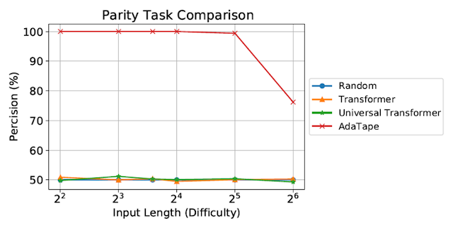
We evaluate AdaTape on parity, a very challenging task for the standard Transformer, to study the effect of inductive biases in AdaTape. With the parity task, given a sequence 1s, 0s, and -1s, the model has to predict the evenness or oddness of the number of 1s in the sequence. Parity is the simplest non-counter-free or periodic regular language, but perhaps surprisingly, the task is unsolvable by the standard Transformer.

Evaluation on the parity task. The standard Transformer and Universal Transformer were unable to perform this task, both showing performance at the level of a random guessing baseline.

Despite being evaluated on short, simple sequences, both the standard Transformer and Universal Transformers were unable to perform the parity task as they are unable to maintain a counter within the model. However, AdaTape outperforms all baselines, as it incorporates a lightweight recurrence within its input selection mechanism, providing an inductive bias that enables the implicit maintenance of a counter, which is not possible in standard Transformers.


Evaluation on image classification

We also evaluate AdaTape on the image classification task. To do so, we trained AdaTape on ImageNet-1K from scratch. The figure below shows the accuracy of AdaTape and the baseline methods, including A-ViT, and the Universal Transformer ViT (UViT and U2T) versus their speed (measured as number of images, processed by each code, per second). In terms of quality and cost tradeoff, AdaTape performs much better than the alternative adaptive transformer baselines. In terms of efficiency, larger AdaTape models (in terms of parameter count) are faster than smaller baselines. Such results are consistent with the finding from previous work that shows that the adaptive model depth architectures are not well suited for many accelerators, like the TPU.

We evaluate AdaTape by training on ImageNet from scratch. For A-ViT, we not only report their results from the paper but also re-implement A-ViT by training from scratch, i.e., A-ViT(Ours).

A study of AdaTape’s behavior

In addition to its performance on the parity task and ImageNet-1K, we also evaluated the token selection behavior of AdaTape with an input-driven bank on the JFT-300M validation set. To better understand the model's behavior, we visualized the token selection results on the input-driven bank as heatmaps, where lighter colors mean that position is more frequently selected. The heatmaps reveal that AdaTape more frequently picks the central patches. This aligns with our prior knowledge, as central patches are typically more informative — especially in the context of datasets with natural images, where the main object is in the middle of the image. This result highlights the intelligence of AdaTape, as it can effectively identify and prioritize more informative patches to improve its performance.

We visualize the tape token selection heatmap of AdaTape-B/32 (left) and AdaTape-B/16 (right). The hotter / lighter color means the patch at this position is more frequently selected.

Conclusion

AdaTape is characterized by elastic sequence lengths generated by the adaptive tape reading mechanism. This also introduces a new inductive bias that enables AdaTape to have the potential to solve tasks that are challenging for both standard transformers and existing adaptive transformers. By conducting comprehensive experiments on image recognition benchmarks, we demonstrate that AdaTape outperforms standard transformers and adaptive architecture transformers when computation is held constant.


Acknowledgments

One of the authors of this post, Mostafa Dehghani, is now at Google DeepMind.

Source: Google AI Blog


Multimodal medical AI

Medicine is an inherently multimodal discipline. When providing care, clinicians routinely interpret data from a wide range of modalities including medical images, clinical notes, lab tests, electronic health records, genomics, and more. Over the last decade or so, AI systems have achieved expert-level performance on specific tasks within specific modalities — some AI systems processing CT scans, while others analyzing high magnification pathology slides, and still others hunting for rare genetic variations. The inputs to these systems tend to be complex data such as images, and they typically provide structured outputs, whether in the form of discrete grades or dense image segmentation masks. In parallel, the capacities and capabilities of large language models (LLMs) have become so advanced that they have demonstrated comprehension and expertise in medical knowledge by both interpreting and responding in plain language. But how do we bring these capabilities together to build medical AI systems that can leverage information from all these sources?

In today’s blog post, we outline a spectrum of approaches to bringing multimodal capabilities to LLMs and share some exciting results on the tractability of building multimodal medical LLMs, as described in three recent research papers. The papers, in turn, outline how to introduce de novo modalities to an LLM, how to graft a state-of-the-art medical imaging foundation model onto a conversational LLM, and first steps towards building a truly generalist multimodal medical AI system. If successfully matured, multimodal medical LLMs might serve as the basis of new assistive technologies spanning professional medicine, medical research, and consumer applications. As with our prior work, we emphasize the need for careful evaluation of these technologies in collaboration with the medical community and healthcare ecosystem.


A spectrum of approaches

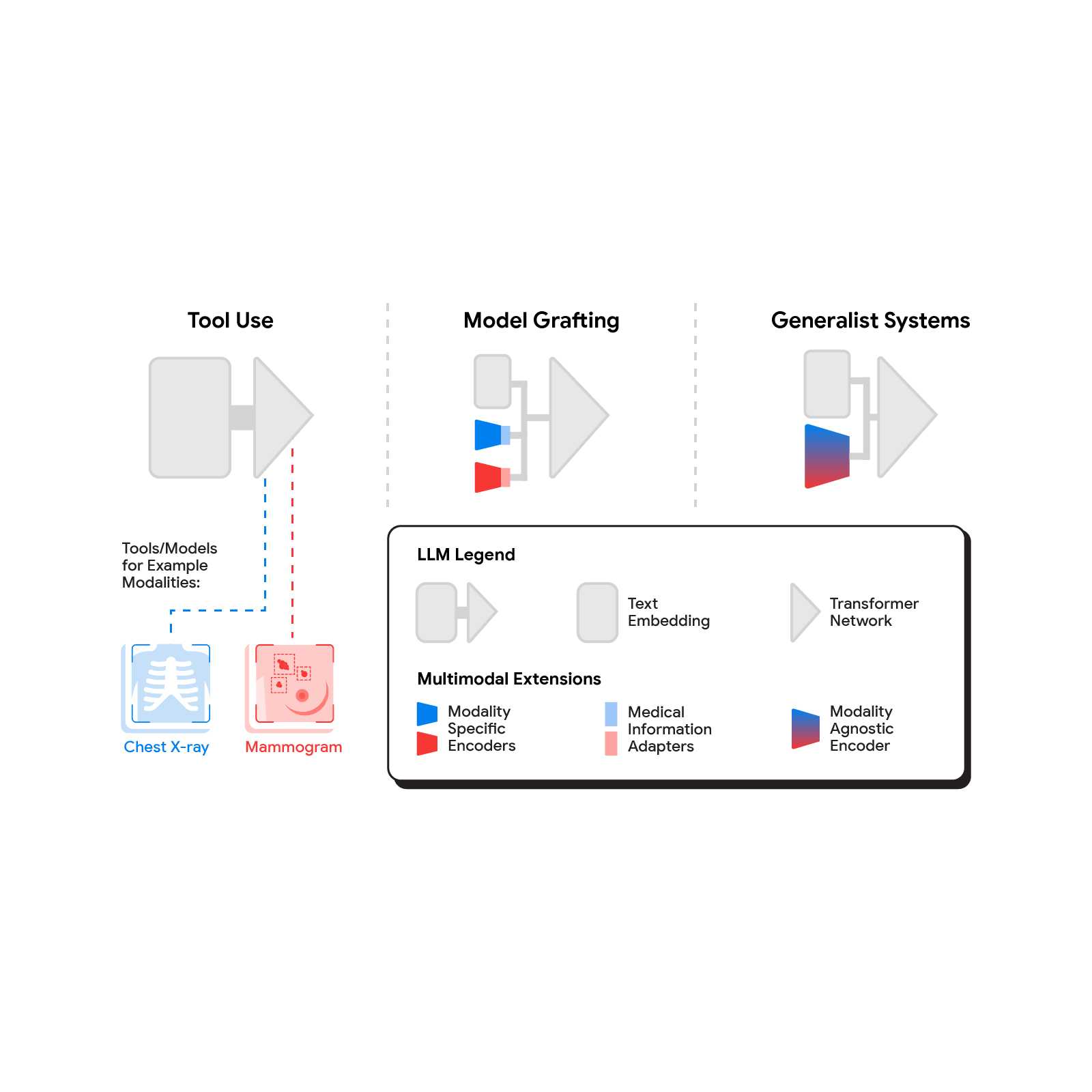
Several methods for building multimodal LLMs have been proposed in recent months [1, 2, 3], and no doubt new methods will continue to emerge for some time. For the purpose of understanding the opportunities to bring new modalities to medical AI systems, we’ll consider three broadly defined approaches: tool use, model grafting, and generalist systems.

The spectrum of approaches to building multimodal LLMs range from having the LLM use existing tools or models, to leveraging domain-specific components with an adapter, to joint modeling of a multimodal model.

Tool use

In the tool use approach, one central medical LLM outsources analysis of data in various modalities to a set of software subsystems independently optimized for those tasks: the tools. The common mnemonic example of tool use is teaching an LLM to use a calculator rather than do arithmetic on its own. In the medical space, a medical LLM faced with a chest X-ray could forward that image to a radiology AI system and integrate that response. This could be accomplished via application programming interfaces (APIs) offered by subsystems, or more fancifully, two medical AI systems with different specializations engaging in a conversation.

This approach has some important benefits. It allows maximum flexibility and independence between subsystems, enabling health systems to mix and match products between tech providers based on validated performance characteristics of subsystems. Moreover, human-readable communication channels between subsystems maximize auditability and debuggability. That said, getting the communication right between independent subsystems can be tricky, narrowing the information transfer, or exposing a risk of miscommunication and information loss.


Model grafting

A more integrated approach would be to take a neural network specialized for each relevant domain, and adapt it to plug directly into the LLM — grafting the visual model onto the core reasoning agent. In contrast to tool use where the specific tool(s) used are determined by the LLM, in model grafting the researchers may choose to use, refine, or develop specific models during development. In two recent papers from Google Research, we show that this is in fact feasible. Neural LLMs typically process text by first mapping words into a vector embedding space. Both papers build on the idea of mapping data from a new modality into the input word embedding space already familiar to the LLM. The first paper, “Multimodal LLMs for health grounded in individual-specific data”, shows that asthma risk prediction in the UK Biobank can be improved if we first train a neural network classifier to interpret spirograms (a modality used to assess breathing ability) and then adapt the output of that network to serve as input into the LLM.

The second paper, “ELIXR: Towards a general purpose X-ray artificial intelligence system through alignment of large language models and radiology vision encoders”, takes this same tack, but applies it to full-scale image encoder models in radiology. Starting with a foundation model for understanding chest X-rays, already shown to be a good basis for building a variety of classifiers in this modality, this paper describes training a lightweight medical information adapter that re-expresses the top layer output of the foundation model as a series of tokens in the LLM’s input embeddings space. Despite fine-tuning neither the visual encoder nor the language model, the resulting system displays capabilities it wasn’t trained for, including semantic search and visual question answering.

Our approach to grafting a model works by training a medical information adapter that maps the output of an existing or refined image encoder into an LLM-understandable form.

Model grafting has a number of advantages. It uses relatively modest computational resources to train the adapter layers but allows the LLM to build on existing highly-optimized and validated models in each data domain. The modularization of the problem into encoder, adapter, and LLM components can also facilitate testing and debugging of individual software components when developing and deploying such a system. The corresponding disadvantages are that the communication between the specialist encoder and the LLM is no longer human readable (being a series of high dimensional vectors), and the grafting procedure requires building a new adapter for not just every domain-specific encoder, but also every revision of each of those encoders.


Generalist systems

The most radical approach to multimodal medical AI is to build one integrated, fully generalist system natively capable of absorbing information from all sources. In our third paper in this area, “Towards Generalist Biomedical AI”, rather than having separate encoders and adapters for each data modality, we build on PaLM-E, a recently published multimodal model that is itself a combination of a single LLM (PaLM) and a single vision encoder (ViT). In this set up, text and tabular data modalities are covered by the LLM text encoder, but now all other data are treated as an image and fed to the vision encoder.

Med-PaLM M is a large multimodal generative model that flexibly encodes and interprets biomedical data including clinical language, imaging, and genomics with the same model weights.

We specialize PaLM-E to the medical domain by fine-tuning the complete set of model parameters on medical datasets described in the paper. The resulting generalist medical AI system is a multimodal version of Med-PaLM that we call Med-PaLM M. The flexible multimodal sequence-to-sequence architecture allows us to interleave various types of multimodal biomedical information in a single interaction. To the best of our knowledge, it is the first demonstration of a single unified model that can interpret multimodal biomedical data and handle a diverse range of tasks using the same set of model weights across all tasks (detailed evaluations in the paper).

This generalist-system approach to multimodality is both the most ambitious and simultaneously most elegant of the approaches we describe. In principle, this direct approach maximizes flexibility and information transfer between modalities. With no APIs to maintain compatibility across and no proliferation of adapter layers, the generalist approach has arguably the simplest design. But that same elegance is also the source of some of its disadvantages. Computational costs are often higher, and with a unitary vision encoder serving a wide range of modalities, domain specialization or system debuggability could suffer.


The reality of multimodal medical AI

To make the most of AI in medicine, we’ll need to combine the strength of expert systems trained with predictive AI with the flexibility made possible through generative AI. Which approach (or combination of approaches) will be most useful in the field depends on a multitude of as-yet unassessed factors. Is the flexibility and simplicity of a generalist model more valuable than the modularity of model grafting or tool use? Which approach gives the highest quality results for a specific real-world use case? Is the preferred approach different for supporting medical research or medical education vs. augmenting medical practice? Answering these questions will require ongoing rigorous empirical research and continued direct collaboration with healthcare providers, medical institutions, government entities, and healthcare industry partners broadly. We look forward to finding the answers together.

Source: Google AI Blog


Announcing the first Machine Unlearning Challenge

Deep learning has recently driven tremendous progress in a wide array of applications, ranging from realistic image generation and impressive retrieval systems to language models that can hold human-like conversations. While this progress is very exciting, the widespread use of deep neural network models requires caution: as guided by Google’s AI Principles, we seek to develop AI technologies responsibly by understanding and mitigating potential risks, such as the propagation and amplification of unfair biases and protecting user privacy.

Fully erasing the influence of the data requested to be deleted is challenging since, aside from simply deleting it from databases where it’s stored, it also requires erasing the influence of that data on other artifacts such as trained machine learning models. Moreover, recent research [1, 2] has shown that in some cases it may be possible to infer with high accuracy whether an example was used to train a machine learning model using membership inference attacks (MIAs). This can raise privacy concerns, as it implies that even if an individual's data is deleted from a database, it may still be possible to infer whether that individual's data was used to train a model.

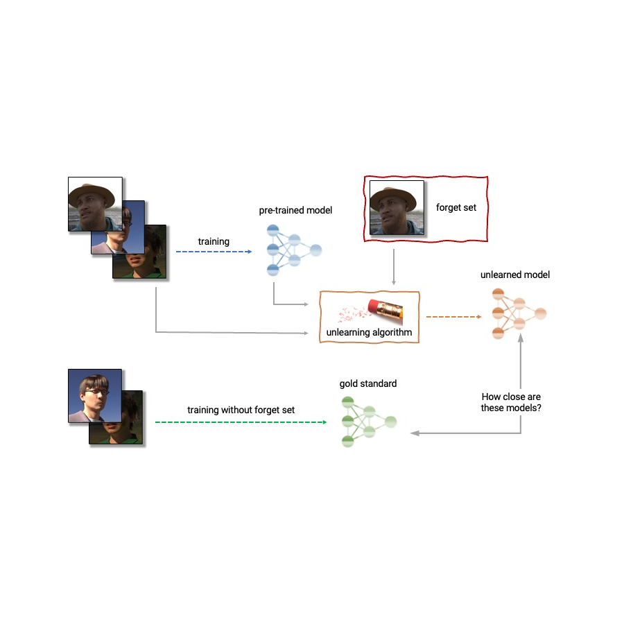
Given the above, machine unlearning is an emergent subfield of machine learning that aims to remove the influence of a specific subset of training examples — the "forget set" — from a trained model. Furthermore, an ideal unlearning algorithm would remove the influence of certain examples while maintaining other beneficial properties, such as the accuracy on the rest of the train set and generalization to held-out examples. A straightforward way to produce this unlearned model is to retrain the model on an adjusted training set that excludes the samples from the forget set. However, this is not always a viable option, as retraining deep models can be computationally expensive. An ideal unlearning algorithm would instead use the already-trained model as a starting point and efficiently make adjustments to remove the influence of the requested data.

Today we're thrilled to announce that we've teamed up with a broad group of academic and industrial researchers to organize the first Machine Unlearning Challenge. The competition considers a realistic scenario in which after training, a certain subset of the training images must be forgotten to protect the privacy or rights of the individuals concerned. The competition will be hosted on Kaggle, and submissions will be automatically scored in terms of both forgetting quality and model utility. We hope that this competition will help advance the state of the art in machine unlearning and encourage the development of efficient, effective and ethical unlearning algorithms.


Machine unlearning applications

Machine unlearning has applications beyond protecting user privacy. For instance, one can use unlearning to erase inaccurate or outdated information from trained models (e.g., due to errors in labeling or changes in the environment) or remove harmful, manipulated, or outlier data.

The field of machine unlearning is related to other areas of machine learning such as differential privacy, life-long learning, and fairness. Differential privacy aims to guarantee that no particular training example has too large an influence on the trained model; a stronger goal compared to that of unlearning, which only requires erasing the influence of the designated forget set. Life-long learning research aims to design models that can learn continuously while maintaining previously-acquired skills. As work on unlearning progresses, it may also open additional ways to boost fairness in models, by correcting unfair biases or disparate treatment of members belonging to different groups (e.g., demographics, age groups, etc.).

Anatomy of unlearning. An unlearning algorithm takes as input a pre-trained model and one or more samples from the train set to unlearn (the "forget set"). From the model, forget set, and retain set, the unlearning algorithm produces an updated model. An ideal unlearning algorithm produces a model that is indistinguishable from the model trained without the forget set.

Challenges of machine unlearning

The problem of unlearning is complex and multifaceted as it involves several conflicting objectives: forgetting the requested data, maintaining the model’s utility (e.g., accuracy on retained and held-out data), and efficiency. Because of this, existing unlearning algorithms make different trade-offs. For example, full retraining achieves successful forgetting without damaging model utility, but with poor efficiency, while adding noise to the weights achieves forgetting at the expense of utility.

Furthermore, the evaluation of forgetting algorithms in the literature has so far been highly inconsistent. While some works report the classification accuracy on the samples to unlearn, others report distance to the fully retrained model, and yet others use the error rate of membership inference attacks as a metric for forgetting quality [4, 5, 6].

We believe that the inconsistency of evaluation metrics and the lack of a standardized protocol is a serious impediment to progress in the field — we are unable to make direct comparisons between different unlearning methods in the literature. This leaves us with a myopic view of the relative merits and drawbacks of different approaches, as well as open challenges and opportunities for developing improved algorithms. To address the issue of inconsistent evaluation and to advance the state of the art in the field of machine unlearning, we've teamed up with a broad group of academic and industrial researchers to organize the first unlearning challenge.


Announcing the first Machine Unlearning Challenge

We are pleased to announce the first Machine Unlearning Challenge, which will be held as part of the NeurIPS 2023 Competition Track. The goal of the competition is twofold. First, by unifying and standardizing the evaluation metrics for unlearning, we hope to identify the strengths and weaknesses of different algorithms through apples-to-apples comparisons. Second, by opening this competition to everyone, we hope to foster novel solutions and shed light on open challenges and opportunities.

The competition will be hosted on Kaggle and run between mid-July 2023 and mid-September 2023. As part of the competition, today we're announcing the availability of the starting kit. This starting kit provides a foundation for participants to build and test their unlearning models on a toy dataset.

The competition considers a realistic scenario in which an age predictor has been trained on face images, and, after training, a certain subset of the training images must be forgotten to protect the privacy or rights of the individuals concerned. For this, we will make available as part of the starting kit a dataset of synthetic faces (samples shown below) and we'll also use several real-face datasets for evaluation of submissions. The participants are asked to submit code that takes as input the trained predictor, the forget and retain sets, and outputs the weights of a predictor that has unlearned the designated forget set. We will evaluate submissions based on both the strength of the forgetting algorithm and model utility. We will also enforce a hard cut-off that rejects unlearning algorithms that run slower than a fraction of the time it takes to retrain. A valuable outcome of this competition will be to characterize the trade-offs of different unlearning algorithms.

Excerpt images from the Face Synthetics dataset together with age annotations. The competition considers the scenario in which an age predictor has been trained on face images like the above, and, after training, a certain subset of the training images must be forgotten.

For evaluating forgetting, we will use tools inspired by MIAs, such as LiRA. MIAs were first developed in the privacy and security literature and their goal is to infer which examples were part of the training set. Intuitively, if unlearning is successful, the unlearned model contains no traces of the forgotten examples, causing MIAs to fail: the attacker would be unable to infer that the forget set was, in fact, part of the original training set. In addition, we will also use statistical tests to quantify how different the distribution of unlearned models (produced by a particular submitted unlearning algorithm) is compared to the distribution of models retrained from scratch. For an ideal unlearning algorithm, these two will be indistinguishable.


Conclusion

Machine unlearning is a powerful tool that has the potential to address several open problems in machine learning. As research in this area continues, we hope to see new methods that are more efficient, effective, and responsible. We are thrilled to have the opportunity via this competition to spark interest in this field, and we are looking forward to sharing our insights and findings with the community.


Acknowledgements

The authors of this post are now part of Google DeepMind. We are writing this blog post on behalf of the organization team of the Unlearning Competition: Eleni Triantafillou*, Fabian Pedregosa* (*equal contribution), Meghdad Kurmanji, Kairan Zhao, Gintare Karolina Dziugaite, Peter Triantafillou, Ioannis Mitliagkas, Vincent Dumoulin, Lisheng Sun Hosoya, Peter Kairouz, Julio C. S. Jacques Junior, Jun Wan, Sergio Escalera and Isabelle Guyon.

Source: Google AI Blog


Visual captions: Using large language models to augment video conferences with dynamic visuals

Recent advances in video conferencing have significantly improved remote video communication through features like live captioning and noise cancellation. However, there are various situations where dynamic visual augmentation would be useful to better convey complex and nuanced information. For example, when discussing what to order at a Japanese restaurant, your friends could share visuals that would help you feel more confident about ordering the “Sukiyaki”. Or when talking about your recent family trip to San Francisco, you may want to show a photo from your personal album.

In “Visual Captions: Augmenting Verbal Communication With On-the-fly Visuals”, presented at ACM CHI 2023, we introduce a system that uses verbal cues to augment synchronous video communication with real-time visuals. We fine-tuned a large language model to proactively suggest relevant visuals in open-vocabulary conversations using a dataset we curated for this purpose. We open sourced Visual Captions as part of the ARChat project, which is designed for rapid prototyping of augmented communication with real-time transcription.

Visual Captions facilitates verbal communication with real-time visuals. The system is even robust against typical mistakes that may often appear in real-time speech-to-text transcription. For example, out of context, the transcription model misunderstood the word "pier" as "pair", but Visual Captions still recommends images of the Santa Monica Pier.

Design space for augmenting verbal communication with dynamic visuals

We invited 10 internal participants, each with various technical and non-technical backgrounds, including software engineers, researchers, UX designers, visual artists, students, etc., to discuss their particular needs and desires for a potential real-time visual augmentation service. In two sessions, we introduced low-fidelity prototypes of the envisioned system, followed by video demos of the existing text-to-image systems. These discussions informed a design space with eight dimensions for visual augmentation of real-time conversations, labeled below as D1 to D8.

Visual augmentations could be synchronous or asynchronous with the conversation (D1: Temporal), could be used for both expressing and understanding speech content (D2: Subject), and could be applied using a wide range of different visual content, visual types, and visual sources (D3: Visual). Such visual augmentation might vary depending on the scale of the meetings (D4: Scale) and whether a meeting is in co-located or remote settings (D5: Space). These factors also influence whether the visuals should be displayed privately, shared between participants, or public to everyone (D6: Privacy). Participants also identified different ways in which they would like to interact with the system while having conversations (D7: Initiation). For example, people proposed different levels of “proactivity”, which indicates the degree to which users would like the model to take the initiative. Finally, participants envisioned different methods of interaction, for example, using speech or gestures for input. (D8: Interaction).

Design space for augmenting verbal communication with dynamic visuals.

Informed by this initial feedback, we designed Visual Captions to focus on generating synchronous visuals of semantically relevant visual content, type, and source. While participants in these initial exploratory sessions were participating in one-to-one remote conversations, deployment of Visual Captions in the wild will often be in one-to-many (e.g., an individual giving a presentation to an audience) and many-to-many scenarios (e.g., a discussion among multiple people in a meeting).

Because the visual that best complements a conversation depends strongly on the context of the discussion, we needed a training set specific to this purpose. So, we collected a dataset of 1595 quadruples of language (1), visual content (2), type (3), and source (4) across a variety of contexts, including daily conversations, lectures, and travel guides. For example, “I would love to see it!” corresponds to visual content of “face smiling”, a visual type of “emoji”, and visual source of “public search”. “Did she tell you about our trip to Mexico?” corresponds to visual content of “a photo from the trip to Mexico'', a visual type of “photo”, and visual source of “personal album”. We publicly released this VC1.5K dataset for the research community.


Visual intent prediction model

To predict what visuals could supplement a conversation, we trained a visual intent prediction model based on a large language model using the VC1.5K dataset. For training, we parsed each visual intent into the format of "<Visual Type> of <Visual Content> from <Visual Source>".

{"prompt": "<Previous Two Sentences> →", 
  "completion": 
"<Visual Type 1> of "<Visual Type 1> from "<Visual Source 1>;
 <Visual Type 2> of "<Visual Type 2> from "<Visual Source 2>; 
  ... \𝑛"}

Using this format, this system can handle open-vocabulary conversations and contextually predict visual content, visual source, and visual type. Anecdotally, we found that it outperforms keyword-based approaches, which fail to handle open-vocabulary examples like “Your aunt Amy will be visiting this Saturday,” and cannot suggest relevant visual types or visual sources.

Examples of visual intent predictions by our model.

We used 1276 (80%) examples from the VC1.5K dataset for fine-tuning the large language model and the remaining 319 (20%) examples as test data. We measured the performance of the fine-tuned model with the token accuracy metric, i.e., the percentage of tokens in a batch that were correctly predicted by the model. During training, our model reached a training token accuracy of 97% and a validation token accuracy of 87%.


Performance

To evaluate the utility of the trained Visual Captions model, we invited 89 participants to perform 846 tasks. They were asked to provide feedback on a scale of "1 — Strongly Disagree" to "7 — Strongly Agree" for six qualitative statements. Most participants preferred to have the visual during a conversation (Q1, 83% ≥ 5–Somewhat Agree). Moreover, they considered the displayed visuals to be useful and informative (Q2, 82% ≥ 5–Somewhat Agree), high-quality (Q3, 82% ≥ 5–Somewhat Agree), and relevant to the original speech (Q4, 84% ≥ 5–Somewhat Agree). Participants also found the predicted visual type (Q5, 87% ≥ 5–Somewhat Agree) and visual source (Q6, 86% ≥ 5–Somewhat Agree) to be accurate given the context of the corresponding conversation.

Technical evaluation results of the visual prediction model rated by study participants.

With this fine-tuned visual intent prediction model, we developed Visual Captions on the ARChat platform, which can add new interactive widgets directly on the camera streams of video conferencing platforms, such as Google Meet. As shown in the system workflow below, Visual Captions automatically captures the user's speech, retrieves the last sentences, feeds them into the visual intent prediction model every 100 ms, retrieves relevant visuals, and then suggests visuals in real time.

System workflow of Visual Captions.

Visual Captions provides three levels of proactivity when suggesting visuals:

  • Auto-display (high-proactivity): The system autonomously searches and displays visuals publicly to all meeting participants. No user interaction required.
  • Auto-suggest (medium-proactivity): The suggested visuals are shown in a private scrolling view. A user then clicks a visual to display it publicly. In this mode, the system is proactively recommending visuals, but the user decides when and what to display.
  • On-demand-suggest (low-proactivity): The system will only suggest visuals if a user presses the spacebar.

Quantitative and qualitative evaluation: User studies

We evaluated Visual Captions in both a controlled lab study (n = 26) and in-the-wild deployment studies (n = 10). Participants found that real-time visuals facilitated live conversations by helping explain unfamiliar concepts, resolve language ambiguities, and make conversations more engaging. Participants also reported different preferences for interacting with the system in-situ, and that varying levels of proactivity were preferred in different social scenarios.

Participants’ Task Load Index and Likert scale ratings (from 1 - Strongly Disagree to 7 - Strongly Agree) of four conversations without Visual Captions (“No VC”) and the three Visual Captions modes: auto-display, auto-suggest, and on-demand suggest.

Conclusions and future directions

This work proposes a system for real-time visual augmentation of verbal communication, called Visual Captions, that was trained using a dataset of 1595 visual intents collected from 246 participants, covering 15 topic categories. We publicly release the training dataset, VC1.5K to the research community to support further research in this space. We have also deployed Visual Captions in ARChat, which facilitates video conferences in Google Meet by transcribing meetings and augmenting the camera video streams.

Visual Captions represents a significant step towards enhancing verbal communication with on-the-fly visuals. By understanding the importance of visual cues in everyday conversations, we can create more effective communication tools and improve how people connect.


Acknowledgements

This work is a collaboration across multiple teams at Google. Key contributors to the project include Xingyu “Bruce” Liu, Vladimir Kirilyuk, Xiuxiu Yuan, Peggy Chi, Alex Olwal, and Ruofei Du.

We would like to extend our thanks to those on the ARChat team who provided assistance, including Jason Mayes, Max Spear, Na Li, Jun Zhang, Jing Jin, Yuan Ren, Adarsh Kowdle, Ping Yu, Darcy Philippon, and Ezgi Oztelcan. We would also like to thank the many people with whom we've had insightful discussions and those who provided feedback on the manuscript, including Eric Turner, Yinda Zhang, Feitong Tan, Danhang Tang, and Shahram Izadi. We would also like to thank our CHI reviewers for their insightful feedback.

Source: Google AI Blog


Resolving code review comments with ML

Code-change reviews are a critical part of the software development process at scale, taking a significant amount of the code authors’ and the code reviewers’ time. As part of this process, the reviewer inspects the proposed code and asks the author for code changes through comments written in natural language. At Google, we see millions of reviewer comments per year, and authors require an average of ~60 minutes active shepherding time between sending changes for review and finally submitting the change. In our measurements, the required active work time that the code author must do to address reviewer comments grows almost linearly with the number of comments. However, with machine learning (ML), we have an opportunity to automate and streamline the code review process, e.g., by proposing code changes based on a comment’s text.

Today, we describe applying recent advances of large sequence models in a real-world setting to automatically resolve code review comments in the day-to-day development workflow at Google (publication forthcoming). As of today, code-change authors at Google address a substantial amount of reviewer comments by applying an ML-suggested edit. We expect that to reduce time spent on code reviews by hundreds of thousands of hours annually at Google scale. Unsolicited, very positive feedback highlights that the impact of ML-suggested code edits increases Googlers' productivity and allows them to focus on more creative and complex tasks.


Predicting the code edit

We started by training a model that predicts code edits needed to address reviewer comments. The model is pre-trained on various coding tasks and related developer activities (e.g., renaming a variable, repairing a broken build, editing a file). It’s then fine-tuned for this specific task with reviewed code changes, the reviewer comments, and the edits the author performed to address those comments.

An example of an ML-suggested edit of refactorings that are spread within the code.

Google uses a monorepo, a single repository for all of its software artifacts, which allows our training dataset to include all unrestricted code used to build Google's most recent software, as well as previous versions.

To improve the model quality, we iterated on the training dataset. For example, we compared the model performance for datasets with a single reviewer comment per file to datasets with multiple comments per file, and experimented with classifiers to clean up the training data based on a small, curated dataset to choose the model with the best offline precision and recall metrics.


Serving infrastructure and user experience

We designed and implemented the feature on top of the trained model, focusing on the overall user experience and developer efficiency. As part of this, we explored different user experience (UX) alternatives through a series of user studies. We then refined the feature based on insights from an internal beta (i.e., a test of the feature in development) including user feedback (e.g., a “Was this helpful?” button next to the suggested edit).

The final model was calibrated for a target precision of 50%. That is, we tuned the model and the suggestions filtering, so that 50% of suggested edits on our evaluation dataset are correct. In general, increasing the target precision reduces the number of shown suggested edits, and decreasing the target precision leads to more incorrect suggested edits. Incorrect suggested edits take the developers time and reduce the developers’ trust in the feature. We found that a target precision of 50% provides a good balance.

At a high level, for every new reviewer comment, we generate the model input in the same format that is used for training, query the model, and generate the suggested code edit. If the model is confident in the prediction and a few additional heuristics are satisfied, we send the suggested edit to downstream systems. The downstream systems, i.e., the code review frontend and the integrated development environment (IDE), expose the suggested edits to the user and log user interactions, such as preview and apply events. A dedicated pipeline collects these logs and generates aggregate insights, e.g., the overall acceptance rates as reported in this blog post.

Architecture of the ML-suggested edits infrastructure. We process code and infrastructure from multiple services, get the model predictions and surface the predictions in the code review tool and IDE.

The developer interacts with the ML-suggested edits in the code review tool and the IDE. Based on insights from the user studies, the integration into the code review tool is most suitable for a streamlined review experience. The IDE integration provides additional functionality and supports 3-way merging of the ML-suggested edits (left in the figure below) in case of conflicting local changes on top of the reviewed code state (right) into the merge result (center).

3-way-merge UX in IDE.

Results

Offline evaluations indicate that the model addresses 52% of comments with a target precision of 50%. The online metrics of the beta and the full internal launch confirm these offline metrics, i.e., we see model suggestions above our target model confidence for around 50% of all relevant reviewer comments. 40% to 50% of all previewed suggested edits are applied by code authors.

We used the “not helpful” feedback during the beta to identify recurring failure patterns of the model. We implemented serving-time heuristics to filter these and, thus, reduce the number of shown incorrect predictions. With these changes, we traded quantity for quality and observed an increased real-world acceptance rate.

Code review tool UX. The suggestion is shown as part of the comment and can be previewed, applied and rated as helpful or not helpful.

Our beta launch showed a discoverability challenge: code authors only previewed ~20% of all generated suggested edits. We modified the UX and introduced a prominent “Show ML-edit” button (see the figure above) next to the reviewer comment, leading to an overall preview rate of ~40% at launch. We additionally found that suggested edits in the code review tool are often not applicable due to conflicting changes that the author did during the review process. We addressed this with a button in the code review tool that opens the IDE in a merge view for the suggested edit. We now observe that more than 70% of these are applied in the code review tool and fewer than 30% are applied in the IDE. All these changes allowed us to increase the overall fraction of reviewer comments that are addressed with an ML-suggested edit by a factor of 2 from beta to the full internal launch. At Google scale, these results help automate the resolution of hundreds of thousands of comments each year.

Suggestions filtering funnel.

We see ML-suggested edits addressing a wide range of reviewer comments in production. This includes simple localized refactorings and refactorings that are spread within the code, as shown in the examples throughout the blog post above. The feature addresses longer and less formally-worded comments that require code generation, refactorings and imports.

Example of a suggestion for a longer and less formally worded comment that requires code generation, refactorings and imports.

The model can also respond to complex comments and produce extensive code edits (shown below). The generated test case follows the existing unit test pattern, while changing the details as described in the comment. Additionally, the edit suggests a comprehensive name for the test reflecting the test semantics.

Example of the model's ability to respond to complex comments and produce extensive code edits.

Conclusion and future work

In this post, we introduced an ML-assistance feature to reduce the time spent on code review related changes. At the moment, a substantial amount of all actionable code review comments on supported languages are addressed with applied ML-suggested edits at Google. A 12-week A/B experiment across all Google developers will further measure the impact of the feature on the overall developer productivity.

We are working on improvements throughout the whole stack. This includes increasing the quality and recall of the model and building a more streamlined experience for the developer with improved discoverability throughout the review process. As part of this, we are investigating the option of showing suggested edits to the reviewer while they draft comments and expanding the feature into the IDE to enable code-change authors to get suggested code edits for natural-language commands.


Acknowledgements

This is the work of many people in Google Core Systems & Experiences team, Google Research, and DeepMind. We'd like to specifically thank Peter Choy for bringing the collaboration together, and all of our team members for their key contributions and useful advice, including Marcus Revaj, Gabriela Surita, Maxim Tabachnyk, Jacob Austin, Nimesh Ghelani, Dan Zheng, Peter Josling, Mariana Stariolo, Chris Gorgolewski, Sascha Varkevisser, Katja Grünwedel, Alberto Elizondo, Tobias Welp, Paige Bailey, Pierre-Antoine Manzagol, Pascal Lamblin, Chenjie Gu, Petros Maniatis, Henryk Michalewski, Sara Wiltberger, Ambar Murillo, Satish Chandra, Madhura Dudhgaonkar, Niranjan Tulpule, Zoubin Ghahramani, Juanjo Carin, Danny Tarlow, Kevin Villela, Stoyan Nikolov, David Tattersall, Boris Bokowski, Kathy Nix, Mehdi Ghissassi, Luis C. Cobo, Yujia Li, David Choi, Kristóf Molnár, Vahid Meimand, Amit Patel, Brett Wiltshire, Laurent Le Brun, Mingpan Guo, Hermann Loose, Jonas Mattes, Savinee Dancs.

Source: Google AI Blog